7 Tesla fMRI Reveals Systematic Functional Organization for Binocular Disparity in Dorsal Visual Cortex
←
→
Page content transcription
If your browser does not render page correctly, please read the page content below
3056 • The Journal of Neuroscience, February 18, 2015 • 35(7):3056 –3072

Systems/Circuits

7 Tesla fMRI Reveals Systematic Functional Organization for
Binocular Disparity in Dorsal Visual Cortex
Nuno R. Goncalves,1 Hiroshi Ban,2,3 Rosa M. Sánchez-Panchuelo,4 Susan T. Francis,4 Denis Schluppeck,5
and Andrew E. Welchman1
1Department of Psychology, University of Cambridge, Cambridge, CB2 3EB, United Kingdom, 2Center for Information and Neural Networks, National
Institute of Information and Communications Technology, Suita City, Osaka, 565-0871, Japan, 3Graduate School of Frontier Biosciences, Osaka University,
Suita City, Osaka 565-0871, Japan, and 4Sir Peter Mansfield Magnetic Resonance Centre, School of Physics and Astronomy, and 5Visual Neuroscience
Group, School of Psychology, University of Nottingham, Nottingham NG7 2RD, United Kingdom

The binocular disparity between the views of the world registered by the left and right eyes provides a powerful signal about the depth
structure of the environment. Despite increasing knowledge of the cortical areas that process disparity from animal models, compara-
tively little is known about the local architecture of stereoscopic processing in the human brain. Here, we take advantage of the high
spatial specificity and image contrast offered by 7 tesla fMRI to test for systematic organization of disparity representations in the human
brain. Participants viewed random dot stereogram stimuli depicting different depth positions while we recorded fMRI responses from
dorsomedial visual cortex. We repeated measurements across three separate imaging sessions. Using a series of computational modeling
approaches, we report three main advances in understanding disparity organization in the human brain. First, we show that disparity
preferences are clustered and that this organization persists across imaging sessions, particularly in area V3A. Second, we observe
differences between the local distribution of voxel responses in early and dorsomedial visual areas, suggesting different cortical organi-
zation. Third, using modeling of voxel responses, we show that higher dorsal areas (V3A, V3B/KO) have properties that are characteristic
of human depth judgments: a simple model that uses tuning parameters estimated from fMRI data captures known variations in human
psychophysical performance. Together, these findings indicate that human dorsal visual cortex contains selective cortical structures for
disparity that may support the neural computations that underlie depth perception.
Key words: binocular disparity; fMRI; psychophysics; ultra-high-field imaging; V3A; visual cortex

Introduction                                                                                                                 Here, we investigate the brain organization that may underlie
Understanding cortical organization at the mesoscopic scale is an                                                        our ability to make precise depth judgments based on binocular
important step in characterizing local neural circuits. The hyper-                                                       disparities. Extracting depth from disparity is a demanding, yet
column concept (Hubel and Wiesel, 1974) has been extremely                                                               routine, neural computation, making it plausible that it is sup-
influential in modeling cortical functional architecture (Ts’o et                                                        ported by systematically organized cortical structures. Record-
al., 2001) and provides a framework to test the neural machinery                                                         ings from cat and macaque cortex indicate that neighborhoods
that facilitates sensory processing. However, despite good knowl-                                                        respond similarly to disparity; that is, electrophysiology and op-
edge from animal models, comparatively little is known about the                                                         tical imaging showed that disparity populations are structured in
local architecture of human cortex.                                                                                      V2 (Hubel and Livingstone, 1987; Roe and Ts’o, 1995; Ts’o et al.,
                                                                                                                         2001; Chen et al., 2008; Kara and Boyd, 2009), V3/V3A (Adams
                                                                                                                         and Zeki, 2001; Anzai et al., 2011; Hubel et al., 2013), and MT/V5
Received July 23, 2014; revised Dec. 24, 2014; accepted Dec. 30, 2014.                                                   (DeAngelis and Newsome, 1999). In contrast, area V1 is reported
   Author contributions: N.R.G., H.B., R.M.S.-P., S.T.F., D.S., and A.E.W. designed research; N.R.G., H.B., R.M.S.-P.,   to show, at best, weak clustering (LeVay and Voigt, 1988; Prince
S.T.F., D.S., and A.E.W. performed research; N.R.G., H.B., D.S., and A.E.W. analyzed data; N.R.G., H.B., R.M.S.-P.,      et al., 2002b).
S.T.F., D.S., and A.E.W. wrote the paper.
   This work was supported by the European Community’s Seventh Framework Programme FP7/2007-2013 (Grant
                                                                                                                             Tests of disparity processing in the primate brain point to
PITN-GA- 2011-290011), the Japan Society for the Promotion of Science (JSPS KAKENHI Grant 26870911), and the             strong fMRI responses in area V3A (Backus et al., 2001; Tsao et
Wellcome Trust (Grant 095183/Z/10/Z).                                                                                    al., 2003; Preston et al., 2008). This work complements evidence
   The authors declare no competing financial interests.                                                                 that macaque V3A contains clusters of disparity selective neurons
   This article is freely available online through the J Neurosci Author Open Choice option.
   Correspondence should be addressed to Andrew E. Welchman, Department of Psychology, University of Cam-                (Adams and Zeki, 2001; Anzai et al., 2011; Hubel et al., 2013).
bridge, Downing Street, Cambridge CB2 3EB, United Kingdom. E-mail: aew69@cam.ac.uk.                                      Here, we therefore focus on responses to disparity in the dorso-
   DOI:10.1523/JNEUROSCI.3047-14.2015                                                                                    medial region around V3A using human brain imaging. To
Copyright © 2015 Goncalves et al.                                                                                        benefit from improved signal-to-noise and high BOLD contrast-
   This is an Open Access article distributed under the terms of the Creative Commons Attribution License
(http://creativecommons.org/licenses/by/3.0), which permits unrestricted use, distribution and reproduction in           to-noise ratios (van der Zwaag et al., 2009), we used ultra-high
any medium provided that the original work is properly attributed.                                                       field (UHF) 7 tesla (7 T) fMRI. Recent UHF fMRI work indicates
Goncalves et al. • Systematic Functional Organization for Disparity J. Neurosci., February 18, 2015 • 35(7):3056 –3072 • 3057
that it can link structures observed in animal models with repre- 2 sessions (sessions 1 and 2). These imaging sessions were performed on
sentations in the human brain: organization for ocular domi- different days. In sessions 1 and 2, we presented stimuli at fine-to-
nance and orientation was reported in primary visual cortex intermediate disparity levels (⫾3, 9, and 15 arcmin). In the third session,
(Cheng et al., 2001; Yacoub et al., 2008), whereas structured re- we delivered stimuli at intermediate-to-coarse disparities (⫾12, 24, and
36 arcmin).
sponses to motion direction were observed in area MT/V5 (Zim-
BOLD responses to binocular disparity were estimated using a block
mermann et al., 2011).
design. During each block, stimuli were presented at one of the six dis-
We report that human visual cortex is systematically orga- parity levels defined for that session. The block length was 15 s, with 10
nized for binocular disparity, with dorsomedial area (V3A/B) stimuli presented for 1 s with an interstimulus interval of 0.5 s. During a
showing structure that relates to the functional characteristics of run, six different blocks were presented (one for each disparity level) and
depth perception. First, we test for clustering of disparity re- each was repeated three times (18 blocks). In addition, there was a fixa-
sponse profiles, finding evidence for maps that are reproducible tion block at the start and the end of each run. Each run lasted 300 s (20
across imaging sessions. We then characterize the selectivity of blocks ⫻ 15 s) and we collected eight or nine functional runs in each
individual voxels for disparities of different magnitudes. We find imaging session. On each run, we asked participants to fixate in the
different profiles of voxel responses: some show fine-tuned re- central fixation square while performing a Vernier detection task (Pres-
sponses whereas others have categorical responses (i.e., near vs ton et al., 2008).
Imaging. Imaging sessions were performed at the Sir Peter Mansfield
far depth). By fitting Gabor models to voxel profiles, we show a
Magnetic Resonance Centre, University of Nottingham, on a 7 T Philips
relationship between the magnitude of disparity and the tuning Achieva scanner with volume transmit and a 32-channel receive coil.
width of voxels in V3A and V3B/KO, but not earlier visual areas. Head motion was restricted by the use of foam padding and a vacuum
Finally, we demonstrate a similarity between these voxel re- pillow (B.u.W. Schmidt). Data were acquired using a 3D gradient echo
sponses and established models of the functional properties of echoplanar imaging [3D GE-EPI with SENSE factor 2.35 in the anterior–
human stereopsis. Together, our findings suggest that dorsal vi- posterior (AP) direction and 2 in the foot-head (FH) direction, TE/TR ⫽
sual cortex (V3A, V3B/KO) contains specialized organization for 28/82 ms, FA ⫽ 22°, EPI factor 45; 0.96 ⫻ 0.96 ⫻ 1 mm 3; matrix size:
disparity, which may support the neural computations underly- 160 ⫻ 160 ⫻ 36 (AP ⫻ RL ⫻ FH); volume acquisition time of 3 s; 100
ing 3D perception. volumes per run] to acquire blood oxygen level-dependent signals from
a field of view (FOV) spanning the dorsomedial visual cortex. The
reduced FOV required the use of outer-volume suppression in the
Materials and Methods phase encoding direction (AP) to prevent signal foldover. We assessed
Participants. Six subjects (three male, aged 25–38 years, including au- signal quality by contrasting all presented stimuli against fixation and
thors N.R.G., H.B., A.E.W.) participated in the study. Participants pro- found no reliable differences in signal quality between the separate
vided informed consent and procedures were approved by the University imaging sessions.
of Nottingham Medical School Ethics Committee. All participants had Before 7 T imaging sessions, participants underwent localizer scans at
normal or corrected-to-normal vision and did not present stereo deficits. the Birmingham University Imaging Centre (BUIC). A 3 T Philips
One participant (Participant 5) withdrew from the study after the second Achieva scanner was used to collect fMRI data to standard retinotopy
scan. experiments (Preston et al., 2008). Retinotopic maps were later used to
Stimuli and design. Stimuli were presented stereoscopically using red define regions of interest (ROIs) and to assist in positioning the acquisi-
and green anaglyphs (the very tight confines of the head coil meant that tion volume over dorsomedial visual areas for 7 T data acquisition. An
other stereoscopic display techniques were not feasible). Participants anatomical volume was also acquired (MPRAGE, 1 mm isotropic reso-
viewed stimuli projected onto a screen located at their feet (viewing lution) and used for surface reconstruction using FreeSurfer (Dale et al.,
distance ⫽ 242 cm). To view the screen from within the head coil, they 1999; Fischl et al., 1999). The resulting reconstructed white matter (WM)
wore prism glasses (to which the red and green filters of the anaglyphs and gray matter (GM) surfaces were then used to compute cortical pro-
were attached). Stimuli were rear-projected onto the display screen from files. These cortical profiles were defined as vectors that connect corre-
an Epson EMP-8300NL using a Nivitar NuView long-throw lens. At the sponding vertices in WM and GM surfaces. These vectors were then used
start of each scan session, we verified the correspondence between dis- to sample functional data at different relative depths.
parity sign (e.g., “negative”) in software with that presented on the pro- We analyzed functional data using mrTools (http://www.cns.nyu.
jection screen (i.e., perceptually “near”): an experimenter viewed the edu/heegerlab) and custom MATLAB code (The Mathworks). We first
screen from the front while wearing the prism glasses with anaglyph coregistered functional scans to the anatomical volume used for surface
filters attached. reconstruction and subsequent analyses were performed in the individ-
Stimuli consisted of random dot stereograms (7° ⫻ 7°) on a midgray ual native space. Preprocessing consisted of motion correction using
background surrounded by a static grid of black and white squares in- linear interpolation and linear detrending. We modeled the BOLD signal
tended to facilitate stable vergence. Dots in the stereogram followed a using the six disparity levels as regressors of interest and estimated the
black or white Gaussian luminance profile, subtending 0.07° at half max- model parameters (i.e., the -weights) associated with each condition.
imum. There were 108 dots/deg 2, resulting in ⬃38% coverage of the Voxel preference was assigned on a “winner-take-all” basis with respect
background. In the center of the stereogram, 4 wedges were equally dis- to the magnitude of the -weights across conditions. Voxel disparity
tributed around a circular aperture (1.2°), each subtending 3° in the preferences were mapped onto the cortical surface by sampling the func-
radial direction and 70° in polar angle, with a 20° gap between wedges tional data (nearest neighbor interpolation) at intermediate depths along
(Fig. 1A). We varied the depth of the wedges by modulating disparity a cortical profile. Although measurements at UHF are less susceptible to
levels in relation to the fixation point (3, 9, 12, 15, 24, and 36 arcmin ⫾ vascular influences (Gati et al., 1997; Ogawa et al., 1998; Uğurbil et al.,
0.5 arcmin jitter, crossed and uncrossed). At a given time point, all 2003), sampling at intermediate depths further minimizes the influence
wedges presented the same disparity. To reduce adaptation, we ap- of superficial veins (Sánchez-Panchuelo et al., 2012) and improves spatial
plied a random polar rotation to the set of wedges such that the localization (Polimeni et al., 2010). Nevertheless, we also quantified vas-
disparity edges of the stimuli were in different locations for each cular influences by calculating the mean BOLD signal amplitude across
stimulus presentation (i.e., a rigid body rotation of the four depth the cortical surface.
wedges together around the fixation point). In the center of the wedge Multivoxel pattern analysis. To confirm that our target regions carried
field, we presented a fixation square (side length ⫽ 1°) paired with information about the stimulus dimension that we manipulated, we used
horizontal and vertical nonius lines. standard multivariate analyses on activity from retinotopically defined
Four participants underwent 3 imaging sessions (Participants 1, 2, 3, areas in dorsomedial visual cortex (Preston et al., 2008). For each ROI, we
and 6) and the remaining participants (Participants 4 and 5) took part in converted voxel time series to z-scores and shifted the respective time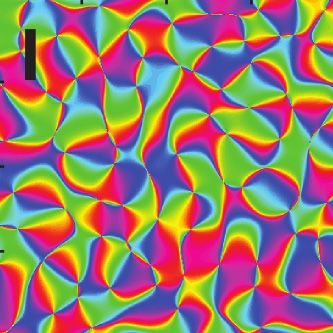
3058 • J. Neurosci., February 18, 2015 • 35(7):3056 –3072                                                                                  Goncalves et al. • Systematic Functional Organization for Disparity

Figure 1. Schematic illustration of the stimuli and basic functional activations. A, Diagram of the depth arrangement in the stimuli. Four disparity-defined wedges were simultaneously presented
at 1 of 6 disparity-defined depths during each imaging session (⫾3, 9, and 15 arcmin in sessions 1 and 2; ⫾12, 24, and 36 arcmin in Session 3). B, The depth of the wedges was defined by
manipulating disparity in random dot stereograms, which were viewed through red-green anaglyphs attached to prism glasses. C, BOLD signals were acquired from dorsomedial visual cortex. Slice
placement is illustrated here on a near midsagittal slice in Participant 1. D, Signal changes in response to stimulus delivery (stimulus vs rest) for Participant 1, showing that activity is localized to the
gray matter. E, Mean percent-signal change for stimulation versus blank periods across all subjects and sessions (N ⫽ 16). Error bars represent the SEM. F, Mean prediction accuracy for the
discrimination of crossed “near” versus uncrossed “far” disparities across early and dorsal visual areas (two-way classification). Chance level (50%) is indicated by the dashed gray line. Error bars
depict the SEM across subjects and sessions (N ⫽ 16). G, Mean prediction accuracy for the discrimination of individual disparity conditions presented within each session (six-way classification).
Chance performance (16.7%) is indicated by the dashed gray line. Error bars depict the SEM across subjects and sessions (N ⫽ 16).

course by 2 volumes (equivalent to 6 s) to account for the hemodynamic                                   hood of voxels surrounding a given target voxel. We first subdivided the
delay. We then averaged data points within each condition block and                                      data into two independent sets (one to find the disparity preference of the
used a linear classifier (support vector machine, libsvm toolbox; Chang                                  target, the other to find the preference of the surround) using a leave-
and Lin, 2011) to discriminate between different stimulus conditions.                                    two-runs-out cross-validation procedure. For each individual voxel, the
We ranked voxels according to the z-score of the comparison between all                                  disparity preference was estimated by fitting a general linear model
stimuli and the fixation blocks and then used the top 500 voxels in each                                 (GLM) to six/seven runs of the total of eight or nine runs acquired. We
ROI for the classification analysis. We followed a leave-one-run-out                                     used the remaining two runs to estimate the disparity preferences of the
cross-validation procedure, resulting in eight or nine folds depending on                                voxels adjacent to the target voxel. Voxels were considered neighbors if
the number of completed runs for each participant (we use the term                                       they belonged to the 26-connected neighborhood that shared a vertex
“fold” to refer to the different combinations of independent subsets of                                  with the target voxel and if they were located within the ROI (e.g., V1)
the data). In particular, from seven/eight runs (of the total eight/nine                                 under consideration. We calculated the frequency of each disparity pref-
runs), we extracted 126/144 patterns to train the classifier and then tested                             erence in the neighborhood of individual voxels and indexed the distri-
the classifier on 18 patterns extracted from the remaining run. This pro-                                bution to the disparity preference of the target voxel. We repeated this
cess was repeated so as to leave out each individual run in turn and the                                 process using different subdivisions of the data for cross-validation
mean accuracy for each subject was computed across folds. We per-                                        (8C2 ⫽ 28 or 9C2 ⫽ 36 folds, depending on the number of experimental
formed two-way (near vs far) and six-way (individual disparities) decod-                                 runs acquired) for each participant and pooled the resulting frequency
ing analysis using this technique.                                                                       distribution across subjects. Frequencies were converted to probabilities
   Calculating the probability of similar voxel preferences in a local neigh-                            by dividing by the total number of adjacent neighbors and then averaged
borhood. To assess the degree of clustering in responses to disparity, we                                according to the preference of the central (target) voxel. This produced
examined the distribution of disparity preferences in the local neighbor-                                six probability distributions that describe disparity preferences in the

Goncalves et al. • Systematic Functional Organization for Disparity J. Neurosci., February 18, 2015 • 35(7):3056 –3072 • 3059
surround of individual voxels (one distribution per central disparity disparity response. We iteratively adjusted an affine transformation W to
preference). To compensate for general biases in disparity preference, we the source map S to minimize the disparity preference difference between
divided each probability distribution by the overall disparity preference corresponding nearest neighbors across sessions, d, which we can define
probability within that ROI. These six relative probability distributions as follows:
were represented in matrix form, where each distribution is represented
by a row vector. Rows indicate the (indexed) central preference and
columns represent the local disparity preference.
d⫽ 冘 i
储R i ⫺ 共 WS 兲 c 共 i 兲 储
Simulating columnar organization and local clustering. To quantify the
where c(i) is the index of the closest voxel of WS in relation to Ri. We
extent to which disparity clustering at the neural level might reasonably
restricted the transformation W to be as small as possible by penalizing
be extracted by a coarser-scale sampling grid (i.e., fMRI voxels), we sim-
large deformations. We thus defined our optimization function as
ulated cortical architectures with different spatial scales and then used
follows:
the clustering analysis described in the previous section. In particular, we
simulated cortical columns of different spatial periodicity by band-pass J ⫽ d ⫹ 储W ⫺ I储
filtering 2D white noise (Rojer and Schwartz, 1990), a method that has
been used previously to simulate orientation columns (Boynton, 2005). where I is the identity matrix and lambda is an empirically defined reg-
We started by generating a matrix in which elements were pseudoran- ularization weight equal to 0.1 that ensured convergence of the minimi-
domly extracted from a normal distribution, representing a 40 mm 2 zation algorithm while preventing gross distortions of the maps. The first
patch of cortex. The noise matrix was band-pass filtered to preserve term of the optimization objective minimizes overall differences in spa-
content with a specific periodicity, which determines the columnar width tial organization of disparity preferences between maps and the second
of the pattern. To test different levels of clustering, we simulated cortical term restricts the spatial transformation to be as small as possible,
columns varying in width between 1 and 4 mm. Having generated the weighted by lambda. The maximum number of iterations was set to 200
neural map, we simulated the fMRI sampling procedure by placing a 2D and the resulting spatial transformations were very close to identity. After
grid of 1 mm squares (representing voxels) over the columnar map. We this alignment step, we recomputed the Pearson correlation coefficient
then assigned a preference to each “voxel” using a probabilistic approach. using bootstrapping (10,000 samples, as above).
In particular, we defined the probability of voxel preference across trials So far, we have described using the Pearson correlation coefficient to
as the distribution of the underlying neural preferences within each quantify the correspondence between disparity maps obtained in differ-
voxel. This provided us with a discrete probability distribution for each ent imaging sessions based on a linear relationship between variables. A
voxel, which we then used to generate 500 fMRI preference maps. We more general approach is to ask how much information is shared be-
then assessed local disparity clustering as above (see “Calculating the tween disparity maps obtained in different imaging sessions. To do so, we
probability of similar voxel preferences in a local neighborhood”). The used mutual information (Shannon, 1948) that quantifies the reduction
only difference was that we considered the 8-connected neighborhood of in uncertainty about a variable after the observation of another variable.
each voxel, as the simulation was performed using a 2D representation, In particular, we computed the reduction in uncertainty about disparity
rather than the 3D data obtained from our empirical measurements. preference in one map after observing the disparity preferences in the
Comparison of disparity preference maps across sessions. To determine other map (note that we performed this analysis on the data without the
whether disparity preferences revealed at the voxel level represented a additional preference alignment step). In the discrete case, mutual infor-
stable property of cortical responses, we sought to compare disparity mation is defined as follows (Shannon and Weaver, 1949):
冘 冉 冊
maps obtained from scans performed on different days. To this end, we
first needed to identify those voxels that had reliable disparity responses PXY 共 x, y兲
I 共 X;Y 兲 ⫽ P XY 共 x, y 兲 log
within each session. We did this by estimating the disparity response of P X 共 x 兲 P Y 共 y兲
x,y
each voxel using a leave-two-runs-out GLM fitting approach. By itera-
tively leaving two runs out, we identified voxels that responded maxi- where PXY (x, y) denotes the joint probability distribution of X and Y and
mally to a given disparity on at least 50% of the GLM fits. Having PX (x) and PY ( y) represent the respective marginal probability distribu-
identified voxels with stable within-session responses, we re-estimated tions. If X and Y are independent, then PXY (x, y) ⫽ PX (x)PY ( y), and
the disparity response of each voxel using the full dataset (i.e., a GLM fit therefore I(X;Y ) ⫽ 0.
to all runs within a session). To coregister maps from different sessions Modeling disparity responses of individual voxels using neuronal tem-
into a common space, we transformed measurements from each partic- plates. To model the responses of individual voxels to different dispari-
ipant’s original functional space to their native anatomical space by ties, we used the disparity tuning templates proposed by Poggio (Poggio
applying the transformation matrix computed during anatomical–func- and Fischer, 1977; Poggio et al., 1988). In particular, we used linear
tional coregistration. We then computed the Pearson correlation be- regression to assess how tuned [tuned near (TN)/tuned far (TF)], cate-
tween corresponding voxels (nearest neighbors) across sessions gorical [near (NE)/far (FA)], and excitatory/inhibitory [tuned excitatory
(bootstrapping, 10,000 samples). To ensure the stability of the correla- (TE)/tuned inhibitory (TI)] cell models explained individual voxel re-
tions, we systematically varied the within-session repeatability criterion sponses. Regressors consisted of discrete ideal responses for each model
(from 50% to 80% of the same preference using the leave-two-runs-out type at the preferred disparity of that voxel and an additional offset/
GLM procedure). We found that our estimates of between-session cor- baseline term. Specifically, the discrete realizations of these models were
relations were stable across this range of within-session repeatability as follows: (1) tuned model, a Kronecker delta shifted to the preferred
thresholds. disparity of the voxel; (2) categorical model, a square wave cycle between
Because the coregistration procedure described above is subject to 0 and 1, odd around zero disparity, so that the positive step coincides
random error, we also used an additional alignment step to compensate with the preferred disparity of the voxel; and (3) excitatory/inhibitory
for small misalignments between data acquired in different sessions. In model, a shifted triangle wave cycle even around zero disparity. The
particular, we recomputed correlations between voxels in different ses- triangle wave had its peak around zero disparity if the disparity prefer-
sions after applying an additional iterative alignment procedure to im- ence of the voxel was the smallest disparity magnitude presented and its
prove coregistration. This procedure adjusted the position of one of the trough otherwise. After assembling the regressors for each voxel, linear
maps to minimize the differences in disparity preference across the ROI regression was performed using MATLAB. This produced a set of four
(we provide results with and without this extra alignment procedure). weights per voxel (one for each tuning model plus the baseline term),
We defined the first session map as the reference and the second session which express the extent to which each model explained the response
map as the source. Let R and S represent the voxels belonging to the profile of individual voxels. For subsequent analysis, we selected voxels
reference and source maps, respectively. Each of these is defined as an that were well modeled by this approach (R 2 ⬎ 0.8).
m-by-four matrix, where m is the number of voxels and each voxel is Modeling voxel responses to disparity using a Gabor model. The previous
described by four features: their 3D coordinates (x, y, z) and their peak section used descriptive neuronal models to examine voxel responses.
3060 • J. Neurosci., February 18, 2015 • 35(7):3056 –3072 Goncalves et al. • Systematic Functional Organization for Disparity
Next, we sought to estimate disparity responses more parametrically. To Gaussian model was insufficient to capture the different profiles of the
this end, we used a 1D Gabor model that has been used to describe the voxels we measured. In particular, 30 (of a total of 60) fits did not pass
response profiles of disparity selective neurons in early and extrastriate the 2 goodness-of-fit test described above ( p ⬍ 0.05). In contrast, using
visual areas (e.g., V1, Prince et al., 2002b; V3/V3A, Anzai et al., 2011; MT, the Gabor model only four of 60 fits failed this test. The superiority of the
DeAngelis and Uka, 2003). In particular, we used a Gabor function to Gabor model was also confirmed using a hold-out cross-validation pro-
describe the response of voxels to variations of binocular disparity. For cedure in which half the data were used to fit the model and the other half
each voxel, we started by removing baseline differences in -weights by used to compute the mean squared error around the fit. This is perhaps
subtracting the mean -weight across all of the presented disparities. For not surprising because the Gabor model has more free parameters than
each ROI, we then grouped voxels based on their preferred disparity (i.e., the Gaussian. Therefore, we also compared these models using the
maximum -weight), resulting in 60 groups (12 preferred disparities for Akaike information criterion (AIC) and found that the mean AIC value
five ROIs). We then fit a Gabor model to each group of voxels (using the across all fits was much lower for the Gabor model. We therefore adopted
data from all the voxels, rather than the averaged voxel response), where the Gabor model to describe the response profiles of our sampled voxels.
the response to a disparity, d, was defined as follows:
Using fMRI-based estimates to model disparity population characteris-
共 d⫺d 0 兲 2 tics. The modeling methods so far described allow us to describe proper-
G 共 d 兲 ⫽ A 0 ⫹ Ae ⫺ 22 cos 共2f 共d ⫺ d0兲 ⫹ 兲 ties of disparity-selective populations based on our fMRI recordings.
Next, we investigated whether these estimates could be related to the
where A is the amplitude, A0 is the baseline, d0 is the position of the characteristics of neural populations that underlie psychophysical depth
Gaussian envelope, is the width of the envelope, f is the frequency of the judgments. Specifically, modeling and psychophysical investigations
cosine, and is the phase shift between the cosine and the center of point to a relationship between disparity selectivity and disparity magni-
the Gaussian envelope. We used constrained optimization (fmincon,
tude: as disparity magnitude increases, disparity detectors are thought to
MATLAB) to find the parameters of the Gabor model that best described
have larger receptive field sizes (Lehky and Sejnowski, 1990; Stevenson et
each group of voxel responses (least-squares estimation). We con-
al., 1992) and this relationship is well approximated by a linear increase
strained the minimizers ad hoc to sensible values given the disparity levels
for disparities (5–20 arcmin) near fixation (Stevenson et al., 1992). Mo-
we presented, which ranged from ⫺36 to 36 arcmin. First, because base-
line correction was performed before fitting, we constrained the baseline tivated by these findings, we investigated whether the envelope size of the
shift to values between ⫺1 and 1. Second, because voxels were grouped fitted Gabor models increased with disparity magnitude. In particular,
by their preferred disparity before fitting, the position of the Gaussian we examined whether there is a correlation between the SD and pre-
was constrained to a window of 10 arcmin around the preferred disparity ferred disparity in each ROI (Pearson’s correlation, p ⬍ 0.05). If the
of each voxel group. Third, the amplitude of the Gaussian envelope was correlation was significant, we used linear regression to estimate the
constrained to 1.2 times the amplitude range of voxel responses and the best fitting trend that describes the variation of each Gabor parameter
width of the Gaussian was restricted between 5 and 12 arcmin to avoid as a function of disparity magnitude; otherwise, the Gabor parameters
overfitting the data. Finally, the frequency was allowed to vary between 0 were assumed to be constant and set to the mean value across dispar-
and 1/(dmax ⫺ dmin) cycles per arcmin, where dmax and dmin represent the ity magnitudes.
maximum and minimum disparity presented during the experimental We centered this analysis on the relationship between the SD of the
session, respectively. This constrained the frequency to remain below half Gaussian envelope and disparity magnitude because we were interested
the sampling frequency. Using these parameter limits enabled us to avoid in changes in response profile width. The parameters of the cosine term
gross overfitting that can arise from the oscillatory term of the Gabor (a (i.e., the frequency f and phase ) provide insight into disparity selectiv-
combination of envelope width and frequency of the carrier). We quan- ity in terms of the presence of on-off subregions within a neuron’s recep-
tified overfitting by contrasting the Gabor model fit against a piecewise tive field. However, in our case, the limited number of disparities
linear fit to neighboring points in the response profile. In particular, we sampled and the aggregated nature of the voxel measurements meant
started by estimating the slope of the line that connects two consecutive that it would be difficult to draw any strong conclusions from any ob-
points of the response profile. Next, we computed the maximum instan- served relationship between these parameters; therefore, we limited our
taneous variation of the fitted Gabor within the same interval and sub- analysis to the relationship between the peak response and SD.
tracted the slope of the linear fit. If the Gabor oscillates considerably Using the estimates of the relationship between disparity magnitude
between two consecutive points, there will be a large absolute difference and envelope size, we built a distributed population of disparity selective
between the maximum variation of the Gabor and the slope computed by units. Here, the term “unit” describes a disparity detector, which, in this
linear approximation. In contrast, if the Gabor follows the linear trajec- case, is derived from a population of voxels. For each ROI, the regression
tory between two consecutive points closely, this difference will be nearly
fits were used to build Gabor detector units at 17 equally spaced disparity
zero.
magnitudes between ⫺40 and 40 arcmin. We then simulated the ability
Using the constraints described above, the optimization function
of this bank of detectors to discriminate different disparities (for a thor-
found good fits across experimental conditions. Specifically, we assessed
ough description, see Lehky and Sejnowski, 1990). In short, we estimated
the quality of fits using a 2 goodness-of-fit test (DeAngelis and Uka,
2003). This test compares the variance of the residuals around the mean the smallest disparity difference that could elicit a significant change in
tuning profile with the variance of the residuals around the model fit. In activity across the population as a whole. First, we computed the re-
particular, we computed the difference between each datum and the sponses of each Gabor unit to two disparity levels and derived the respec-
model value at that disparity, which provided us with a distribution of tive variances assuming direct proportionality. Specifically, if we let Rij be
residuals around the model. We then compared the variance of this the response of unit i to stimulus j, its variance is then given by ij2 ⫽ kRij
distribution against the variance of the residuals around the mean using with k ⫽ 1.5 (for plausibility of this arbitrary parameter, see Lehky and
a 2 test for equal variances. The fit is considered satisfactory if the Sejnowski, 1990). The number of SDs separating these responses was
variances of these distributions do not differ significantly. defined as follows:
The constraints of fMRI data acquisition meant that we were limited in
the number of different disparities that we could measure reliably during 兩R i1 ⫺ Ri2兩
d⬘i ⫽
each imaging session. Therefore, fits to voxel responses are limited in
their resolution along the disparity domain. This presents a challenge in
冑 i12 ⫹ i22
choosing and fitting the correct model to the data. Based on the electro-
physiological literature, a Gabor model is a good descriptor of individual Large values of d⬘i suggest that changes in response of the ith unit were
neuron responses within the visual cortex (see above). As an alternative, stimulus induced, whereas small values indicate chance fluctuations due
we also considered a Gaussian model that has the advantage of fewer to noise. Statistically, the probability of observing a stimulus-induced
parameters. However, comparison of the models indicated that the change in individual units was defined as follows: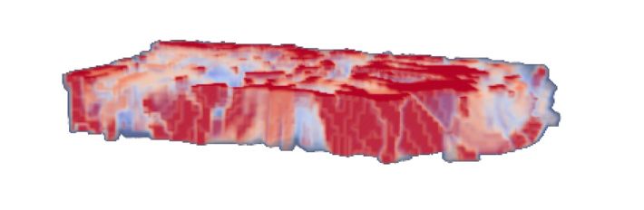
Goncalves et al. • Systematic Functional Organization for Disparity J. Neurosci., February 18, 2015 • 35(7):3056 –3072 • 3061
A C
D
B
Figure 2. Spatial distribution of peak disparity responses in area V3A for two participants. A, Peak disparity responses in left V3A of Participants 1 and 2 (first session). The peak disparity response
of each voxel is mapped onto flattened representations of the cortex. Dark and light gray areas represent sulci and gyri, respectively. Peak disparity responses were sampled from three intermediate
layers of the cortical sheet (at relative depths of 0.4, 0.5, and 0.6) and averaged across depths. B, Mean BOLD signal amplitude in the same ROIs. Dark areas indicate areas of low absolute signal in
the EPI images, and are likely to represent large veins. The white dashed line represents the outline of left V3A shown above. Gray dashed lines delineate areas with low signal amplitude in both maps.
Coarse clusters of peak disparity responses do not overlap with the potential location of large veins. C, The same ROI in Participant 2, but now represented across 11 relative points through the entire
range of the cortical sheet (0 to 1 relative depth, sampled at increments of 0.1). The flattened representations for each cortical depth were stacked together and an opacity gradient was applied to
aid visualization of peak disparity response across the cortical depth. Note that to assist visualization the cortical depth, dimension is not drawn to scale. D, Sliced view of peak disparity responses in
the same ROI (Participant 2, left V3A). Data are cut through the cortical depth along a line extending from the foveal representation of V3A up to the periphery near the border with V3d.
冕
d⬘
were, on average, highest in V3A and at accuracy levels compa-
2 ⫺x/ 2 rable to previous work (Preston et al., 2008). We also performed
pi ⫽ e dx ⫺ 1
冑2 a six-way classification analysis of the data, testing how well the
⫺⬁ presented disparity could be predicted from the six different
At the population level, however, each unit represents one of many di- types of stimuli (i.e., disparity values) presented. We observed
mensions. In this multidimensional space, assuming uncorrelated noise, performance well above chance, with highest mean performance
variations in responses were tested using the joint probability as follows: in V3A (Fig. 1G). These results are consistent with previous work
at 3 T in suggesting strong responses to disparity, particularly in
写
N
areas V3A and V3B/KO (Backus et al., 2001; Tsao et al., 2003;
p⫽1⫺ 1 ⫺ pi
Preston et al., 2008).
i⫽1
This initial examination of the data is confirmatory. However,
Here, p represents the probability of changes across the whole population our primary interest was not in aggregated voxel responses from
being stimulus induced. We finally computed the disparity discrimina- within different ROIs, but rather whether 7 T fMRI would allow
tion threshold as the minimum disparity difference for which p ⬎ 0.5 (as us to detect and quantify consistent spatial organization of indi-
in Lehky and Sejnwoski, 1990; see their erratum). Discrimination thresh- vidual voxel responses. In our next analyses, we therefore con-
olds were evaluated at disparities between ⫺40 and ⫹40 arcmin.
sider the response profiles of individual voxels as a proxy that
Results summarizes the activity of a neural population centered on the
We presented participants with disparity-defined wedges at a voxel. To this end, we used the -weights of the GLM model fit to
range of different depth positions (Fig. 1 A, B) and recorded the the fMRI time series to determine how the different presented
BOLD signal from voxels spanning the dorsomedial visual cortex stimuli explain the activity of individual voxels. We start by de-
(Fig. 1C). We observed strong BOLD responses to manipulations fining the disparity preference of a voxel as the condition that
of disparity that were well localized to the gray matter (Fig. 1D). yields the highest -weight (i.e., winner-take-all labeling). Later,
To provide a first analysis of these data, we quantified aggregated we consider other models that seek to capture the response pro-
BOLD responses in the dorsal visual cortex using two ap- file of a voxel based on all of the estimated -weights.
proaches. First, we computed the change in the BOLD response
for disparity-defined stimuli relative to the fixation baseline in Spatial clustering of peak responses to disparity
each of the localized ROIs. This revealed large changes in the Motivated by reports of disparity clustering in macaque extrastri-
BOLD signal in V1 and dorsal extrastriate cortex (Fig. 1E), with ate cortex (Anzai et al., 2011; Hubel et al., 2013), we tested for
magnitudes consistent with previous studies at UHF (Hoffmann clustering within the human visual cortex. In particular, we ex-
et al., 2009; van der Zwaag et al., 2009; Polimeni et al., 2010). amined the spatial distribution of disparity responses across the
Second, we quantified responses in different ROIs using a multi- cortical surface by labeling individual voxels according to the
voxel decoding analysis approach for disparity-defined stimuli disparity value that evoked the highest level of fMRI activity (i.e.,
(Preston et al., 2008). In particular, we calculated the accuracy of maximum -weight of the GLM) during each imaging session.
a support vector machine in predicting whether a stimulus was To visualize the data, we color-coded the disparity “preferences”
nearer or farther than the fixation point based on patterns of of individual voxels and mapped them onto flattened represen-
voxel activity. We found high accuracies for discriminating tations of the cortex. This produced cortical maps with an appar-
crossed (“near”) versus uncrossed (“far”) disparity (Fig. 1F ) that ent organization: contiguous spaces across the cortical surface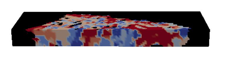
3062 • J. Neurosci., February 18, 2015 • 35(7):3056 –3072 Goncalves et al. • Systematic Functional Organization for Disparity
A B
C D
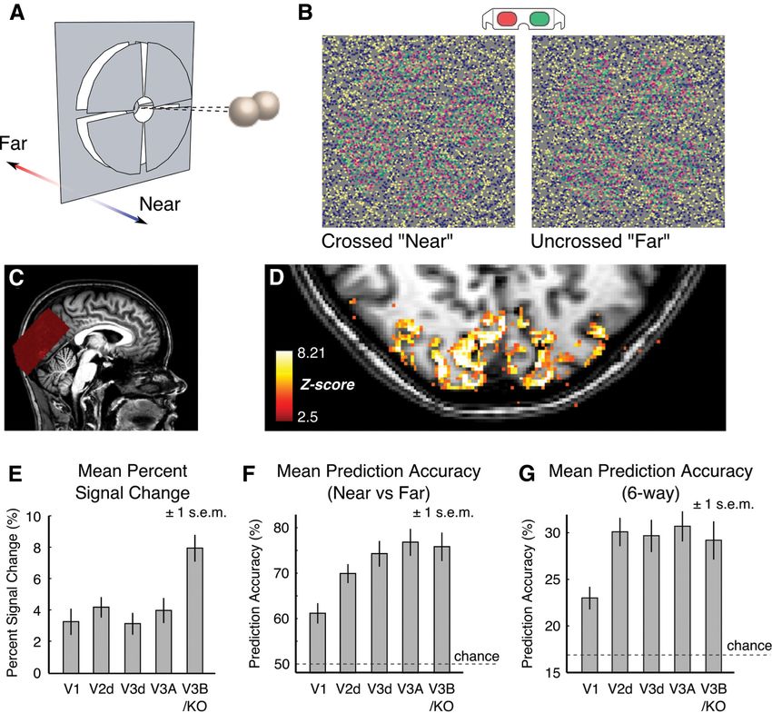
Figure 3. Local clustering of peak voxel responses to disparity (“preferences”) in simulated and empirical datasets. A, Simplified 2D illustration of clustered and disperse preferences for a given
voxel. Individual voxels and their neighbors will often share similar peak responses if there is spatial clustering (top and middle). If there is no organization, no relationship should be observed
between the peak responses of a target voxel and its neighbors (bottom). B, Simulation of columnar architectures for orientation (after Rojer and Schwartz, 1990) with periodicity varying from 1 to
4 mm (top) and the respective preference maps after simulating voxel sampling using six equidistant conditions (middle). Bottom, The correspondence between the preference of target voxels and
their neighborhood is shown in form of a probability matrix for each columnar width. In each matrix, the ith row represents the average probability distribution of preferences around voxels preferring
the ith disparity and the probability value is represented in grayscale (green horizontal line on the color bar indicates chance level, 0.167, given six response options). Maps that are clustered display
a clear diagonal structure, demonstrating that nearby voxels tend to share similar preferences. C, The same matrix representation for empirical disparity maps from visual areas V1, V2d, V3d, V3A,
and V3B/KO. Green horizontal bar on the color bar indicates chance level (0.167). A diagonal structure emerges along the dorsal cortical hierarchy. Note the different grayscale range from part B for
empirical fMRI measurements. D, Results of a similar analysis after randomly shuffling the disparity preferences in V3A and V3B/KO. In this case, we do not observe any diagonal structure.
share similar disparity responses (Fig. 2A). Importantly, these referenced to the disparity preference of the target voxel (see Fig.
contiguous areas did not overlap with regions where the mean 3A for a schematic illustration). Our logical expectation was that
amplitude of the BOLD signal was low, suggesting that clustering if there is clustering in the disparity preferences, target voxels will
was not simply due to macrovasculature (Fig. 2B). Moreover, be surrounded by neighbors with the same (Fig. 3A, top) or sim-
there was reasonable consistency in the peak disparity response at ilar (Fig. 3A, middle) preferences, in contrast to randomly orga-
different cortical depths (Fig. 2C,D; note that the scale of the nized preferences (Fig. 3A, bottom). However, the extent to
cortical depth axis here is expanded relative to the cortical loca- which this structure will be visible depends on the spatial scale of
tion plane to aid visualization). the underlying neural maps in relation to the fMRI sampling
Although these visualizations are useful in illustrating the gen- resolution. Before examining the empirical data, we therefore
eral spatial profiles of responses, the process of mapping and consider the extent to which clustering can be recovered based on
interpolating the data from the (raw) native fMRI data space to a a simulated dataset.
flattened representation of the cortical sheet can introduce over- To test for clustering at the voxel level, we performed simula-
representation (or underrepresentation) of individual datum. In tions using a model of cortical columns for orientation (Rojer
particular, there are frequent one-to-many correspondences be- and Schwartz, 1990) because there is no standard model for dis-
tween voxels in the functional space and pixels visualized on the parity organization. We supposed neural maps of different spatial
flat cortical surface (i.e., oversampling), which can inflate the scales (columns 1– 4 mm in width) and then sampled these maps
extent of clustering observed on these flat maps. Therefore, we using a simulated 1 mm isotropic “voxel” grid (Fig. 3B). There-
sought to evaluate response clustering by examining the disparity after, we computed the voxel similarity of each sampled voxel
response of neighboring voxels in the (native) functional space, relative to its neighbors and then averaged together the neighbor-
thereby ensuring no overrepresentation or underrepresentation hood preferences of all voxels that had the same central voxel
of the data. preference. This resulted in a similarity matrix that shows the
To quantify peak disparity response clustering, we assessed statistical relationship between the preference of central voxels
the similarity between the preference of a central target voxel and relative to their surround (Fig. 3B, bottom), where strong diago-
that of its neighbors. We did this by calculating the distribution of nal structure indicates a close relationship between central voxels
disparity preferences in the population of voxels that shared at and their local neighbors. (Note that the higher probabilities in
least one vertex with the target voxel. Thereby, we calculated a the top left and bottom right corners of these plots arise because
probability map for the disparity preference of the neighborhood orientation is a circular dimension; we would not anticipate theseGoncalves et al. • Systematic Functional Organization for Disparity J. Neurosci., February 18, 2015 • 35(7):3056 –3072 • 3063
for binocular disparity, which is a more linear dimension.) These given location on the cortical sheet, meaning that additional
simulations indicate that, using 1 mm isotropic voxels, it is realistic discrepancies could arise from sampling at different cortical
to obtain information about the structure of underlying cortical or- depths. As a result, we would not necessarily expect one-to-
ganization if the scale of the neural maps is in the region of 3 mm. one voxel correspondence between functional data acquired
This corresponds to the estimated scale of disparity maps in human in different imaging sessions.
cortex based on scaling up measurements from macaque MT to Nevertheless, we were able to capture similarities between
account for overall brain size (DeAngelis and Newsome, 1999, and individual disparity preference maps across sessions for four
see the supplementary information from Ban et al., 2012). of the six participants who took part in repeated sessions (Fig.
Having demonstrated proof of concept, we now return to the 4A–D). In these maps, disparity preferences appear to be
empirical fMRI data. In principle, we could calculate clustering in coarsely organized into bands, which can be clearly identified
exactly the same way as described for the simulations. However, in maps obtained in different imaging sessions (see the out-
real fMRI voxel responses are not temporally or spatially inde- lines in Fig. 4). For one participant (Participant 5; Fig. 4E), we
pendent because of the point-spread function (PSF) of the BOLD found similar structures across sessions but with reversed dis-
signal, meaning that a more sophisticated method is required. In parity sign (note the correspondence between blue and red
particular, we estimated the preference of the central target voxel regions across sessions, particularly in the right hemisphere).
and its neighbors using independent data subsamples (leave-two- This map inversion is consistent with a change from a rear- to
runs-out cross-validation) such that shared preferences for a front- projection setting, causing a left-right horizontal flip
given measurement could not simply be due to the dependency of and thereby reversing the disparity sign presented during the
BOLD responses for nearby voxels. Although this strategy does experiment. We suspect that this was the result of restarting
not remove the influence of spatial blurring, it eliminates tempo- the projector immediately before this participant’s scan due to
ral correlations between neighboring voxels because we use dif- technical problems. For the final participant, we did not find
ferent time courses for estimating the preference of central voxels apparent correspondence between sessions, although we note
and their surround. We computed preference similarity for each that slice positioning was not optimal in the second session
presented disparity value, creating matrices for each ROI (Fig. and a portion of V3A was omitted (Fig. 4F ).
3C). We found that diagonal structure in the preference similar- To quantify the similarity between maps, we used voxelwise
ity matrices became increasingly apparent for measurements at correlation in the native functional space. We first selected voxels
increasing levels of the dorsal cortical hierarchy. To quantify this that had a stable within-session preference and then brought the
observation, we used a reliability statistic that compared the functional data from each session into common alignment (see
mean probability along the positive diagonal of the matrix, with Materials and Methods). We then computed the Pearson corre-
the distribution of mean values calculated from random sam- lation between corresponding voxels (nearest neighbors) across
pling from all locations within the matrix (bootstrapping: 10,000 sessions using bootstrapped resampling (10,000 samples). Con-
resamples of six values). We found evidence for significant clus- firming our observations from the flattened cortical representa-
tering in V2d ( p ⫽ 0.04), V3d ( p ⫽ 0.01), V3A ( p ⫽ 0.02), and tions (Fig. 4), we observed reliable correlations between disparity
V3B/KO ( p ⫽ 0.003), but not in V1 ( p ⫽ 0.11). As a control, we maps for four participants (Fig. 5A, Participants 1– 4). In addi-
recomputed matrices after shuffling disparity preferences and tion, we found reliable negative correlations for one participant
found no systematic structure (Fig. 3D). This confirmed that (Fig. 5A, Participant 5), which is consistent with the apparent
evidence for clustering in higher dorsal areas could not somehow inversion of the disparity maps (Fig. 4E).
derive from differences in size and/or shape of different ROI. As discussed above, small spatial misalignments between ses-
Together, these data provide evidence that clustering of disparity sions can lead to an underestimation of between-session repeat-
preferences is particularly marked in higher dorsal visual areas ability. To ameliorate small misalignments, we considered an
V3A and V3B/KO, in contrast to primary visual cortex. It is pos- additional processing stage in which we incorporated a pre-
sible that preference clustering is much less pronounced in early ference-based between-session alignment step. In particular, we
visual areas. However, recall that, from our simulations of maps calculated an affine transform between the 3D maps that sought
with different spatial scales, it is possible that there is systematic to improve coregistration while minimizing nonlinear deforma-
organization in early areas, but the fMRI sampling resolution tions (see Materials and Methods). We then recomputed corre-
does not allow this to be detected. lations across sessions (Fig. 5B) and found a small improvement
in correlation values for participants with previously reliable
Testing for the reproducibility of disparity responses between-session correspondence. However, the method itself did
The preceding analyses support the notion that responses to dispar- not introduce significant correlations (e.g., Participant 6) when
ity are clustered in dorsal extrastriate cortex. However, to determine there was little common structure before alignment and, in gen-
the extent to which this clustering represents genuine cortical struc- eral, the effect of this additional alignment step was slight. In
ture, we next sought to test whether the spatial distribution of dis- particular, Figure 6 shows the V3A map for Participant 4 (that
parity preferences is a persistent property of neuronal responses. showed the maximum benefit from this alignment step) with and
Specifically, we tested whether preference maps could be reproduced without the additional alignment step.
between different imaging sessions. To provide an additional measure of reproducibility, we com-
Comparing functional data across different imaging ses- puted the mutual information (Shannon, 1948; Shannon and
sions, especially at very high resolution, is extremely challeng- Weaver, 1949) between maps obtained in different imaging ses-
ing and previous UHF studies have therefore focused on sions (using the non-preference-aligned data). We compared the
repeatability within sessions (Cheng et al., 2001; Yacoub et al., empirical mutual information (Fig. 5C) with bootstrapped esti-
2008). In particular, differences in voxel slab positioning in mates based on randomly permuted disparity preferences (Fig.
relation to the cortical sheet affect sampling (Cheng et al., 5C, horizontal lines). We found evidence of persistent informa-
2001). Moreover, with a functional resolution of 1 mm (near tion for five participants, confirming the presence of disparity
isotropic), we expect to acquire approximately 2 points from a selective structures.3064 • J. Neurosci., February 18, 2015 • 35(7):3056 –3072 Goncalves et al. • Systematic Functional Organization for Disparity
A B
C D
E F
Figure 4. Maps of peak disparity responses from area V3A obtained in different imaging sessions. Flattened representations were obtained by averaging disparity preferences across three
intermediate layers in the cortex (0.4, 0.5, and 0.6) so as to avoid distortions caused by macrovasculature near the pial surface. Green pentagrams represent the location of the foveal representation
used to identify the border between area V3A and V3B/KO (using retinotopic mapping). The dorsal direction is indicated by the purple arrow aligned with the vertex of the pentagram. Additional
labels indicate the position of area V3B/KO to aid orientation. A–D, Consistent distribution of disparity responses can be observed in four participants (Participant 1, left V3A; Participant 2, left and
right V3A; Participant 3 right V3A; Participant 4 left V3A). Overlaid contours represent the edges of the uncrossed disparity/”far” (red) region from Session 1. These were calculated by binarizing the
maps and then applying an edge detection algorithm. The outlines were omitted in D (right V3A) because the fine scale changes in this map mean that superimposed contours masked the data and
therefore hindered visualization. E, The distribution of peak disparity responses in Participant 5 reveals similar structures between sessions, but the color map appears to be inverted. F, No
correspondence between disparity maps is evident for Participant 6. Slice positioning in the second session was not optimal, with the result that not all of right hemisphere V3A was fully sampled
(bottom right).You can also read