The temporal structure of the inner retina at a single glance - Nature
←
→
Page content transcription
If your browser does not render page correctly, please read the page content below
www.nature.com/scientificreports

            OPEN           The temporal structure of the inner
                           retina at a single glance
                           Zhijian Zhao1,2,11, David A. Klindt1,2,3,4,5,11, André Maia Chagas1,2,4, Klaudia P. Szatko1,3,4,
                           Luke Rogerson1,2,3,4, Dario A. Protti7, Christian Behrens1,2,3, Deniz Dalkara8, Timm Schubert1,2,
                           Matthias Bethge2,3,5,9, Katrin Franke 1,2,3, Philipp Berens 1,2,3,6, Alexander S. Ecker2,3,5,9,10 &
                           Thomas Euler1,3*
                           The retina decomposes visual stimuli into parallel channels that encode different features of the visual
                           environment. Central to this computation is the synaptic processing in a dense layer of neuropil,
                           the so-called inner plexiform layer (IPL). Here, different types of bipolar cells stratifying at distinct
                           depths relay the excitatory feedforward drive from photoreceptors to amacrine and ganglion cells.
                           Current experimental techniques for studying processing in the IPL do not allow imaging the entire
                           IPL simultaneously in the intact tissue. Here, we extend a two-photon microscope with an electrically
                           tunable lens allowing us to obtain optical vertical slices of the IPL, which provide a complete picture
                           of the response diversity of bipolar cells at a “single glance”. The nature of these axial recordings
                           additionally allowed us to isolate and investigate batch effects, i.e. inter-experimental variations
                           resulting in systematic differences in response speed. As a proof of principle, we developed a simple
                           model that disentangles biological from experimental causes of variability and allowed us to recover
                           the characteristic gradient of response speeds across the IPL with higher precision than before. Our new
                           framework will make it possible to study the computations performed in the central synaptic layer of
                           the retina more efficiently.

                           The primary excitatory pathway of the mouse retina consists of photoreceptors, bipolar cells (BCs) and retinal
                           ganglion cells (RGCs) (reviewed in refs. 1,2). At the core of this pathway is the inner plexiform layer (IPL), a dense
                           synaptic plexus composed of the axon terminals of BCs, the neurites of amacrine cells, as well as the dendrites
                           of RGCs. Specifically, the photoreceptor signal is relayed by the BCs to the RGCs via glutamatergic synapses
                           (reviewed in ref. 3). This “vertical” transmission is shaped by mostly inhibitory interactions with amacrine cells,
                           which integrate signals laterally along and/or vertically across the IPL (reviewed in ref. 4). Amacrine cells modu-
                           late, for instance, the sensitivity of BCs to certain spatio-temporal features5–7.
                               Within the IPL, the axon terminals of each of the 14 BC types8–12 project to a distinct depth with axonal pro-
                           files of different BC types partially overlapping and jointly covering the whole depth of the IPL10,11,13. Functionally,
                           each BC type constitutes a particular feature channel, with certain temporal dynamics7, including On and Off BC
                           types sensitive to light increments or decrements, respectively14, different kinetics15,16, and chromatic signals17,18.
                           Some of these features are systematically mapped across the IPL: For example, On BCs project to the inner and
                           Off BCs to the outer portion of the IPL14,19. Also kinetic response properties appear to be mapped, with the axonal
                           profiles of more transient BCs localised in the IPL centre7,15,20,21.
                               To study BC function, early studies mostly used single-cell electrical recordings in vertical slices, where many
                           lateral connections (e.g. large-scale amacrine cells) are severed, only electrical signals in the cell body of BCs can
                           be recorded and experiments are time consuming. Recently, two-photon (2 P) Ca2+ or glutamate imaging in the
                           explanted whole-mount retina has been introduced as a high-throughput alterative7,15,20. This approach preserves

                           1
                            Institute for Ophthalmic Research, University of Tübingen, Tübingen, Germany. 2Centre for Integrative Neuroscience
                           (CIN), University of Tübingen, Tübingen, Germany. 3Bernstein Centre for Computational Neuroscience, University
                           of Tübingen, Tübingen, Germany. 4Graduate Training Centre of Neuroscience, University of Tübingen, Tübingen,
                           Germany. 5Institute for Theoretical Physics, University of Tübingen, Tübingen, Germany. 6Institute of Bioinformatics
                           and Medical Informatics, University of Tübingen, Tübingen, Germany. 7Department of Physiology and Bosch
                           Institute, The University of Sydney, Sydney, Australia. 8Sorbonne Université, INSERM, CNRS, Institut de la Vision,
                           Paris, France. 9Center for Neuroscience and Artificial Intelligence, Baylor College of Medicine, Houston, TX, USA.
                           10
                              Department of Computer Science, University of Göttingen, Göttingen, Germany. 11These authors contributed
                           equally: Zhijian Zhao and David A. Klindt. *email: thomas.euler@cin.uni-tuebingen.de

Scientific Reports |   (2020) 10:4399 | https://doi.org/10.1038/s41598-020-60214-z                                                               1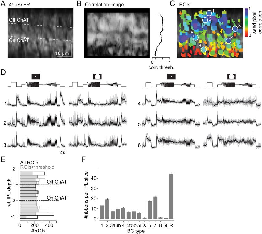
www.nature.com/scientificreports/                                                                                www.nature.com/scientificreports

                               Figure 1. Overview of the two-photon (2 P) microscope equipped with an electrically tunable lens (ETL). For
                               simplicity, most lenses and silver mirrors (M) were omitted. For parts, see Table 1. (A) Schematic diagram of the
                               microscope’s main optical paths, with the EL-16-40-TC (Optotune) inserted before the x-y galvo scan mirrors
                               (MScan). Inset: Cross section and working principle of the ETL; a voice-coil actuator generates pressure on a
                               container, which in turn pushes optic fluid into the lens volume sealed by polymer membrane and, thereby,
                               modulating the curvature of the lens surface. (B) Photograph of the excitation path before the scan mirrors.
                               CM, cold mirror; DM, dichroic mirror; BP, band pass filter; PMT, GaAsP photomultiplier tube; RL, relay lens; T,
                               telescope. Panel A adapted from Euler et al.22, inset adapted from Optotune website (https://www.optotune.com/).

             Part       Description (link)                                                  Company                                Item number (RRID, if available)
                        Electrically tunable large aperture lens https://www.optotune.com
             ETL                                                                            Optotune, Dietikon, Switzerland        EL-16-40-TC-VIS-5D
                        Specification sheet: https://tinyurl.com/EL-16-40-TC
             RL1        Achromatic Doublet, ARC: 650–1050 nm, F = 30 mm                     Thorlabs                               AC254-030-B
             RL2        Achromatic Doublet, ARC: 650–1050 nm, F = 250 mm                    Thorlabs                               AC254-250-B
             RL3        Achromatic Doublet, ARC: 650–1050 nm, F = 80 mm                     Thorlabs                               AC254-080-B
             RL4        Achromatic Doublet, ARC: 650–1050 nm, F = 30 mm                     Thorlabs                               AC127-030-B
             CM         Cold Light Mirror KS 93/45°                                         Qioptiq Photonics                      G380255033
             DM1        Dichroic mirror (custom made)                                       AHF Analysetechnik AG                  F73-063_z400-580-890
             BP1        510/84 BrightLine HC AOI 0°                                         AHF Analysetechnik AG                  F37–584
             BP2        610/75 ET Bandpass AOI 0°                                           AHF Analysetechnik AG                  F49–617
                                                                                            Written by M. Müller (MPI
             ScanM      2 P imaging software running under IGOR Pro
                                                                                            Neurobiology, Martinsried), and T.E.
             IGOR Pro   https://www.wavemetrics.com                                         Wavemetrics, Lake Oswego, OR           IGOR Pro v6 (SCR_000325)
                                                                                            Written by T.E, supported by Tom
             QDSpy      Visual stimulation software https://github.com/eulerlab/QDSpy                                              (SCR_016985)
                                                                                            Boissonnet (EMBL, Monterotondo)

                               Table 1. Parts list.

                               the integrity of the retinal network, but typically requires recording horizontal planes (x-y scans) at different IPL
                               levels. Since the activity at different IPL depths is recorded sequentially, it can be more difficult to disentangle
                               functional differences between the signals represented at different depths and experimental factors inducing dif-
                               ferences between scans.
                                   Here, we introduce fast axial x-z scanning, a method to image across the entire IPL depth near simultaneously
                               in the intact whole-mount retina through “vertical optical slices”, by equipping a 2 P microscope (Fig. 1)22–24 with
                               an electrically tunable lens (ETL) to quickly shift the focus along the z axis25. We evaluated these x-z scans by
                               imaging light stimulus-evoked glutamate release using iGluSnFR26 ubiquitously expressed via AAV transduction.
                               We found that axial x-z scans can capture functional signals at different IPL depths similarly well compared to
                               “traditional” x-y scans7. Because the new scanning mode allowed us to acquire signals with different response
                               polarity and kinetics within a single scan, we were able to identify and correct for batch effects, corresponding to
                               inter-experimental variation caused by experimental and biological factors like indicator concentration and tem-
                               perature. As a proof of principle, we show how correcting for batch effects can markedly improve recovering the
                               characteristic change in response kinetics across the IPL, where fast signals are represented towards the middle
                               and slower signals towards the borders of the IPL7,15,20,27.

Scientific Reports |     (2020) 10:4399 | https://doi.org/10.1038/s41598-020-60214-z                                                                                  2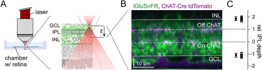
www.nature.com/scientificreports/ www.nature.com/scientificreports
Methods
Equipping the 2 P microscope with an ETL. To allow for axial scanning, we modified a movable objec-
tive microscope (MOM, designed by W. Denk, now MPI Martinsried; purchased from Sutter Instruments/Science
Products, Novato, CA). Design and configuration of the MOM have been described elsewhere7,22,23,28. In brief,
the microscope is driven by a mode-locked Ti:Sapphire laser (MaiTai-HP DeepSee, Newport Spectra-Physics,
Darmstadt, Germany) and equipped with two fluorescence detection channels and a 20x water immersion objec-
tive (W Plan-Apochromat 20×/1.0 DIC M27, Zeiss, Oberkochen, Germany).
An ETL with an open aperture of 16 mm (EL-16-40-TC, Optotune, Dietikon, Switzerland) was introduced into
the laser path before the scanning unit (Fig. 1a); the optical path after the scanners was left unchanged. Before the
ETL, the laser beam is expanded to a diameter of 15 mm using a telescope (T1, a 4f-system with relay lenses RL1,2;
fR1 = 30 mm, fR2 = 250 mm; for complete parts list, see Table 1). The expanded beam is then reflected perpendicularly
to the optical table by a silver mirror towards the horizontally placed ETL, which is housed in a 60 mm cage plate
(Thorlabs, Dachau, Germany) using a custom-made adapter (Fig. 1b). After the laser beam passed the ETL, it is
narrowed by a second telescope (T2, another 4f-system consisting of relay lenses RL3,4; fR3 = 80 mm, fR4 = 30 mm) to
a diameter of approx. 5.6 mm, which approx. matches the size of the scanning mirrors. Telescope T2 relays the pupil
of the ETL to a conjugate pupil on the scan mirrors. Here, RL4 needs to be positioned precisely at its focal distance
and in the centre of the two scan mirrors for correct refocusing of the laser beam. By changing the current supplied
to the ETL, it changes its optical power. According to the EL-16-40-TC’s specifications (see link in Table 1), its optical
power can be tuned from −2 to +3 dioptres (fETL ranging from −500 to 333 mm, for currents of approx. ±250 mA),
rendering the beam divergent or convergent, respectively. Adapting the calculation in Fahrbach et al.29, the shift in
focal plane (Δz, in [µm]) under the objective lens can be roughly estimated using
2 2
f n
2 fSL RL3
∆z = − fObj
water
⋅ 103 ,
fTL fRL 4 fETL (1)
with the focal lengths (in [mm]) of the relay lenses (see above), the scan (fSL = 50) and tube lens (fTL = 200), and
′ ′
refractive index (nwater = 1.333). We estimated the objective’s image-side focal length ( fObj ) using fObj = fRef /MObj
= 8.3 mm, with reference focal length fRef = 165 mm, and magnification MObj = 20×. The object-side focal
′
length ( fObj ) results from the relationship fObj /nwater = fObj /nair , as the objective tip is immersed in solution.
To drive the ETL with our imaging software (ScanM, see below and Table 1), we used custom electronics
(designed by R. Berndt, HIH, Tübingen) that translates a voltage signal from one of the analogue-out channels
of an PCI 6110 card (NI, Austin, US) controlled by ScanM into a stable current signal. To obtain the relationship
between ETL driver input and resulting shift in focal plane, we applied voltage steps of varying amplitude (n =
11 amplitudes, n = 5 trials), presented in a randomized order, and monitored the shift in focal plane by reading
out the z position of the microscope’s motorized scan head. For the used combination of lenses, this resulted in
a measured Δz range of +80 and −120 µm (for ETL driving currents of −100 and +100 mA; cf. Fig. 2B). Due
to technical limitations (i.e. size of the scan mirrors), the Δz range with largely constant laser power spanned
approx. 50 µm (cf. Fig. 2C), which is sufficient to scan across the entire mouse IPL without adapting the laser
power. To characterize the spatial resolution of our system, we measured the point spread function (PSF) of fluo-
rescent beads (170 nm in diameter, λEmission = 515 nm; P7220; Invitrogen) at different axial planes.
Animals and tissue preparation. All animal procedures were approved by the governmental review board
(Regierungspräsidium Tübingen, Baden-Württemberg, Konrad-Adenauer-Str. 20, 72072 Tübingen, Germany)
and performed according to the laws governing animal experimentation issued by the German Government.
For all experiments, we used adult mice of either sex from the following lines: B6;129S6-Chattm2(cre)LowlJ (n = 3;
ChAT:Cre, JAX 006410), and B6;129P2-Pvalbtm1(cre)Arbr/J (n = 6; PV:Cre, JAX 008069). All lines were purchased
from The Jackson Laboratory (Bar Harbor, ME). The transgenic lines were crossbred with the Cre-dependent red
fluorescence reporter line Gt(ROSA)26Sortm9(CAG-tdTomato)Hze (Ai9tdTomato, JAX 007905) for all experiments. Owing
to the exploratory nature of our study, we did not use blinding and did not perform a power analysis to predeter-
mine sample size. For details on the mouse lines and all reagents, see Table 2.
Animals were housed under a standard 12 h day-night cycle. For recordings, animals were dark-adapted
for >1 h, then anaesthetized with isoflurane (Baxter, Deerfield, US) and killed by cervical dislocation. The eyes
were removed and hemisected in carboxygenated (95% O2, 5% CO2) artificial cerebral spinal fluid (ACSF)
solution containing (in mM): 125 NaCl, 2.5 KCl, 2 CaCl2, 1 MgCl2, 1.25 NaH2PO4, 26 NaHCO3, 20 glucose,
and 0.5 L-glutamine (pH 7.4). The tissue was then transferred to the recording chamber of the 2 P microscope,
where it was continuously perfused with carboxygenated ACSF at ∼37 °C. The ACSF contained ∼0.1 µM
sulforhodamine-101 (SR101, Invitrogen, Carlsbad, US) to reveal blood vessels and any damaged cells in the red
fluorescence channel. All procedures were carried out under very dim red (>650 nm) light.
Intravitreal virus injection. For virus injections, mice were anesthetized with 10% ketamine (Bela-Pharm
GmbH & Co. KG, Vechta, Germany) and 2% xylazine (Rompun, Bayer Vital GmbH, Leverkusen, Germany) in
0.9% NaCl (Fresenius, Bad Homburg, Germany). A volume of 1 µl of the viral construct (AAV2.hSyn.iGluSnFR.
WPRE.SV40, Penn Vector Core, Philadelphia, PA, or AAV2.7m8.hSyn.iGluSnFR, produced in D. Dalkara’s lab with
plasmid provided by Jonathan Marvin and Loren Looger, Janelia Research Campus, Ashburn, VA) was injected into
the vitreous humour of both eyes via a Hamilton injection system (syringe: 7634–01, needles: 207434, point style 3,
length 51 mm, Hamilton Messtechnik GmbH, Höchst, Germany) mounted on a micromanipulator (World Precision
Instruments, Sarasota, Germany). Imaging experiments were performed 3 weeks after virus injection.
Scientific Reports | (2020) 10:4399 | https://doi.org/10.1038/s41598-020-60214-z 3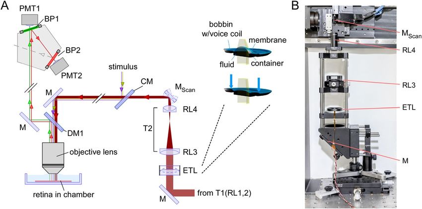
www.nature.com/scientificreports/                                                               www.nature.com/scientificreports

                           Figure 2. Axial scan properties. (A) Illustration of the measurement configuration and the excitation laser’s
                           focus shift (Δz) introduced by the ETL. (B) Axial position (measured with the microscope stage motor) as a
                           function of voltage input to ETL driver (circles represent n = 5 individual measurements per voltage performed
                           in random sequence; dashed curve represents sigmoidal fit). (C) Sulforhodamine 101 (SR101) solution in
                           the chamber was used to measure fluorescence intensity as function of focus shift for two exemplary ETL
                           voltage offsets; x-z scan field (left; 256 × 256 pixels, 2 ms/line; zoomXY,Z = 1.0, 0.8) and mean fluorescence
                           (right). Arrow indicates range (~40 µm) of near-constant fluorescence. Dotted rectangles on the top indicate
                           artefact. (D) Axial x-z scan (64 × 40 pixels, 2 ms/line, zoomXY,Z = 1.0, 1.0, VOffset = 0.15 V) of a 5 μm-thin film
                           of fluorescein solution between two coverslips (measured using the microscopes motorized stage) at different
                           z-positions. After jumping back to the beginning of a frame, the ETL requires a few milliseconds to settle; this
                           “settling” generates an artefact at the bottom of the frame and makes the film appear wider in frame 7 (for
                           details, see Results). Inset: Frame 3 with intensity distribution along z-axis; for this scan configuration, the
                           fluorescent band width was 4.4 pixels ± 0.1 (mean ± s.d. for width at half maximum, n = 5 measurements),
                           corresponding to a pixel “height” of 1.1 µm. (E) Illustration of point spread function (PSF) measurements at
                           three positions (−18 (red), 0 (black), 18 μm (blue)) along the z-axis (right); example images of fluorescent beads
                           (170-nm beads, λEm, Peak = 515 nm; 256 × 256 pixels, n = 60 z-planes, Δz = 0.2 µm, zoomXY = 8) at 0 μm, with
                           mean Gaussian fits (n = 3 measurements/plane). PSFx and PSFz indicate the mean ± s.d. across the three axial
                           planes (n = 9 measurements; see Table 3).

                           Two-photon imaging. We used our microscope’s “green” detection channel (HC 510/84, AHF, Tübingen,
                           Germany) to record iGluSnFR fluorescence, reflecting glutamate signals. In the “red” channel (ET 610/75, AHF),
                           we detected tdTomato to image the ChAT bands (in the ChAT:Cre x Ai9 mice; cf. Fig. 3B) or RGC somata (in the
                           PV:Cre x Ai9 mouse), and SR101 fluorescence to measure fluorescence intensities along the z axis (cf. Fig. 2C).
                           The laser was tuned to 927 nm for all fluorophores. For data acquisition, we used custom software (ScanM, see
                           Table 1) running under IGOR Pro 6.3 for Windows (Wavemetrics, Lake Oswego, US).

                           Light stimulation.         A modified LightCrafter (DLPLCR4500, Texas instruments; modification by EKB
                           Technology) was focused through the objective lens of the microscope22,30. Instead of standard RGB light-emitting
                           diodes (LEDs), it was fitted with a green (576 nm) and a UV (390 nm) LED for matching the spectral sensitivity of
                           mouse M- and S-opsins31,32. To prevent the LEDs from interfering with the fluorescence detection, the light from the
                           projector was band-pass-filtered (ET dual band exciter, 380–407/562–589, AHF) and the LEDs were synchronised
                           with the microscope’s scan retrace23. Stimulator intensity was calibrated to range from 0.1 × 10³ (“black” background
                           image) to 20 × 103 (“white” full field) photoisomerisations P*/s/cone. The light stimulus was centred before every
                           experiment, such that its centre corresponded to the centre of the recording field. Light stimuli were generated using
                           QDSpy, a custom visual stimulation software written in Python 3 (see Table 1). To probe BC function, we presented

Scientific Reports |   (2020) 10:4399 | https://doi.org/10.1038/s41598-020-60214-z                                                             4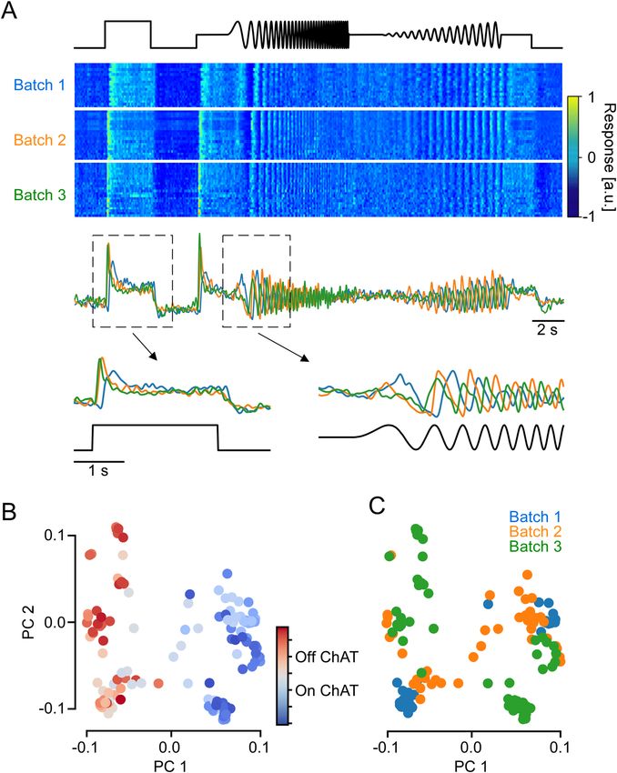
www.nature.com/scientificreports/                                                                                  www.nature.com/scientificreports

                                                                                                                                                           Item
                            Item                                        Description (link)                                            Company              number
                                                                        Mice expressing Cre recombinase in cholinergic neurons,
                            B6;129S6-Chattm2(cre)LowlJ                                                                                Jackson Laboratory   JAX 006410
                                                                        without disrupting endogenous Chat expression
                                                                        Mice expressing Cre recombinase in Pvalb-expressing neurons,
                            B6;129P2-Pvalbtm1(cre)Arbr/J                                                                             Jackson Laboratory    JAX 008069
                                                                        without disrupting endogenous Pvalb expression
                                                                        Mice expressing robust tdTomato fluorescence following Cre-
                            Gt(ROSA)26Sortm9(CAG-tdTomato)Hze                                                                         Jackson Laboratory   JAX 007905
                                                                        mediated recombination
                                                                                                                                      Penn Vector Core,
                            AAV2.hSyn.iGluSnFR.WPRE.SV40                Viral construct
                                                                                                                                      Philadelphia, PA
                                                                        Viral construct, produced in D. Dalkara’s lab with plasmid
                            AAV2.7m8.hSyn.iGluSnFR                      provided by Jonathan Marvin and Loren Looger, Janelia
                                                                        Research Campus, Ashburn, VA
                            NaCl                                        Sodium chloride                                               VWR                  27810.295
                            KCl                                         Potassium chloride                                            Sigma-Aldrich        P9541
                            MgCl2·6H2O                                  Magnesium chloride hexahydrate                                Merck Millipore      1.05833
                            NaH2PO4                                     Sodium phosphate monobasic                                    Sigma-Aldrich        S5011
                            C6H12O6                                     D-(+)-Glucose                                                 Sigma-Aldrich        G8270
                            NaHCO3                                      Sodium hydrogen carbonate                                     Merck Millipore      1.06329
                            CaCl2·2H2O                                  Calcium chloride dihydrate                                    Sigma-Aldrich        C3306
                            C5H10N2O3                                   L-Glutamine                                                   Sigma-Aldrich        G3126
                            SR101                                       sulforhodamine-101                                            Invitrogen           S359

                           Table 2. Mouse lines and reagents.

                            Z position (ETL) [µm]          PSFX [µm]              PSFZ [µm]
                            18                             0.43, 0.42, 0.42       1.98, 2.02, 2.05
                            0                              0.39, 0.37, 0.38       1.78, 1.69, 1.70
                            −18                            0.35, 0.33, 0.38       1.56, 1.62, 1.67

                           Table 3. Point spread functions (PSF) from n = 3 independent measurements at each z position.

                           Figure 3. Mapping the inner plexiform layer (IPL). (A) Illustration of axial scans in the whole-mount retina
                           of a transgenic mouse expressing tdTomato under the ChAT promotor and iGluSnFR via AAV transduction
                           (Methods). (B) Axial x-z scan (256 × 160 pixels, 2 ms/line, zoomXY,Z = 1.5, 0.75) with iGluSnFR expression
                           (green) and ChAT bands (magenta). IPL borders and ChAT bands (solid and dashed lines, respectively) were
                           defined manually (Methods). Note that the retina was flipped from (A), following the convention to show
                           the photoreceptors pointing up. C, IPL border positions relative to ChAT bands (left; INL: 1.9 ± 0.1; GCL:
                           −1.1 ± 0.1; n = 3/6/14 mouse/retinas/scans).

                           3–4 repeats of a “chirp” stimulus in two sizes, local (100 µm in diameter) and global (800 µm); it consisted of a
                           light-On step followed by sinusoidal intensity modulations of increasing frequency and contrasts7.

                           Data analysis. Data preprocessing was performed in IGOR Pro 6 (Wavemetrics), DataJoint33 and Python
                           3. Regions of Interest (ROIs) were defined automatically by custom correlation-based algorithms in IGOR Pro7.
                           First, we estimated a correlation image by correlating the trace of every pixel with the trace of its eight neigh-
                           bouring pixels and calculating the mean local correlation (ρlocal). In contrast to previous x-y recordings7, local
                           correlation of neighbouring pixels varied with IPL depth in x-z scans (Fig. 4B) due to differences in iGluSnFR
                           labelling (Fig. 3B) and laser intensity (Fig. 2C). To account for that, an IPL depth-specific correlation threshold
                           (ρthreshold) was defined as the 70th percentile of all local correlation values in each z-axis scan line. For every pixel

Scientific Reports |   (2020) 10:4399 | https://doi.org/10.1038/s41598-020-60214-z                                                                                      5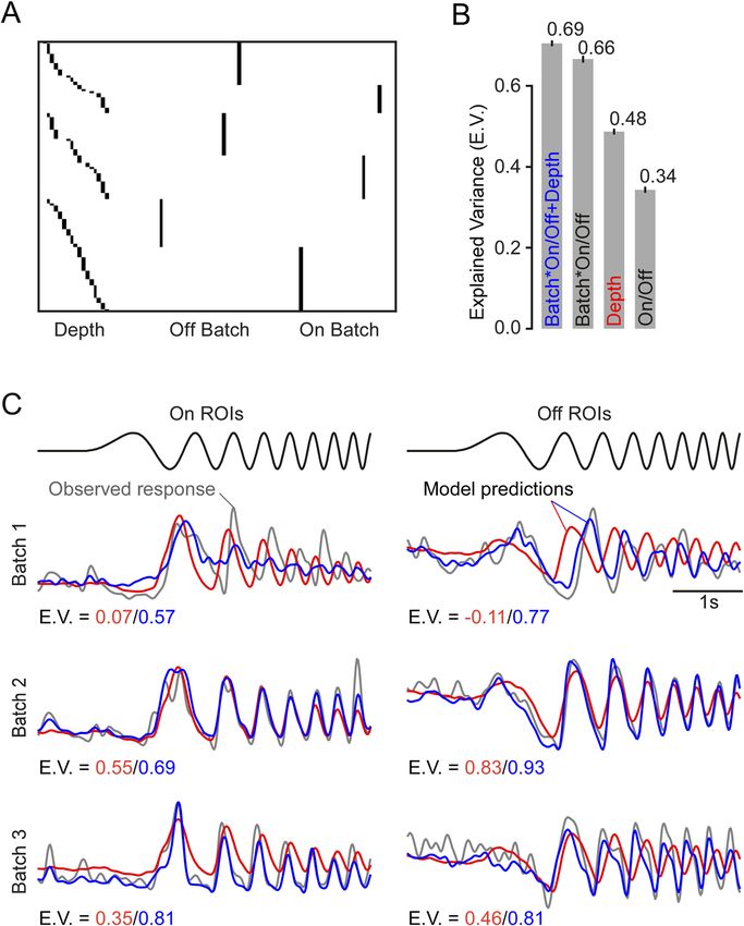
www.nature.com/scientificreports/                                                               www.nature.com/scientificreports

                           Figure 4. Glutamate imaging in the inner plexiform layer. (A) Axial x-z scan (64 × 56 pixels, 1.6 ms/line) of
                           the inner plexiform layer (IPL) in a whole-mount wild-type mouse retina expressing iGluSnFR ubiquitously
                           after AAV-mediated transduction. (B) Correlation image (left) and distribution of correlation thresholds across
                           the IPL (right). (C) ROIs extracted from scan in (A), pseudo-coloured by seed pixel correlation (for details on
                           ROI extraction, see Methods). (D) Glutamate responses to local and global chirp stimulus for exemplary ROIs
                           encircled in (C); Off (left) and On responses (right) are shown. (E) Distribution of all ROIs (black, n = 5,379)
                           and ROIs that passed our quality threshold (grey, n = 3,893; Methods) recorded across the IPL (n = 6/8/37
                           mice/retinas/scans). (F) Number of ribbon synapses from different BC types per vertical IPL slice (Methods),
                           estimated based on available EM data10.

                           with ρlocal > ρthreshold (“seed pixel”), we grouped neighbouring pixels with ρlocal > ρthreshold into one ROI. To match
                           ROI sizes with the sizes of BC axon terminals, we restricted ROI diameters (estimated as effective diameter of
                           area-equivalent circle) to range between 1 and 4 μm.
                              To register each ROI’s depth in the IPL, we determined for each x-z scan the position of the On and the Off
                           ChAT band (Fig. 3; see also Results). In the case of ChAT:Cre x Ai9 mice, ChAT bands could be imaged directly
                           due to their tdTomato fluorescence (Fig. 3B). We found the ChAT band positions can also be reliably deter-
                           mined from the IPL borders, which were determined from the location of iGluSnFR-labelled (or, in PV:Cre x Ai9,
                           tdTomato-labelled) somata in GCL and INL. Here, we first determined the position of the IPL borders relative to
                           tdTomato labelled ChAT bands in a subset of experiments (Fig. 3C). Following conventions34, we defined the On
                           and the Off ChAT band position as 0 and 1, respectively. For every ROI, we then estimated the shortest distance
                           to On and Off ChAT bands or IPL borders and expressed ROI IPL depth as a relative value between approx. −1
                           (GCL border) and +2 (INL border). Next, for every scan field (=batch), ROI depth estimates were corrected
                           using the IPL depth at which the response polarity switched between On and Off BCs. The IPL position of this
                           polarity switch was determined using the first principal component (PC) of the local chirp responses (0.24 ± 0.14,
                           mean ± s.d., n = 37 fields) and subtracted from each scan field’s depth estimates. We then added 0.5 to align the
                           IPL centre, i.e. the separation between On and Off BC terminals to previous definitions34.
                              The glutamate traces for each ROI were extracted using the image analysis toolbox SARFIA for IGOR Pro35.
                           Then, the traces were synchronised to the light stimuli using time markers that were generated by the stimula-
                           tion software and acquired during imaging. Finally, we up-sampled the traces to 64 Hz temporal resolution and
                           de-trended them by applying a high-pass Butterworth filter with a cut-off frequency of 0.1 Hz.

Scientific Reports |   (2020) 10:4399 | https://doi.org/10.1038/s41598-020-60214-z                                                              6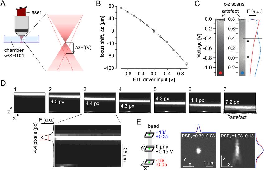
www.nature.com/scientificreports/ www.nature.com/scientificreports
Linear mixed effects model. All modelling was performed using DataJoint and Python 3. Batch effects
were first estimated using a series of simple linear mixed effects models, which predicted the expected glutamate
release of all ROIs across time (Y ∈ NxT , T = 64Hz ⋅ 32s = 2048) as a linear function of different predictors
that were all encoded as dummy variables:
(1) A model that used only the polarity ( X polarity ∈ Nx2) to predict Yˆ = X polarity wpolarity . Thus, this model
computed simply the average of all On and Off ROIs as the weight vector.
(2) A model that used only the IPL depth ( Xdepth ∈ Nx20), where the response is estimated non-parametrical-
ly with 10 depth bins across the IPL for each polarity (cf. Fig. 5A), to predict Ŷ = Xdepthwdepth.
(3) A model that estimated the response of each ROI as a function of the batch ( Xbatch ∈ Nx 2B; B = 36, the
first batch was left out as reference and to avoid a singular design matrix) where each batch had one
predictor per polarity to predict Yˆ = Xbatchwbatch.
(4) And finally, a combined model (2. and 3.) that predicted the response of each ROI as a function of both
batch and depth (Ŷ = Xbatchwbatch + Xdepthwdepth).
In the last model, we wanted to make sure that any shared variance between the two predictors would be
ascribed to the depth predictor – conservatively mistaking nuisance or noise from the batches rather as biological
signal than vice versa. To achieve this, we orthogonalized Xbatch with respect to Xdepth , effectively by using
Xbatch _ new = Xbatch − PdepthXbatch, with Pdepth denoting the projection matrix onto the subspace defined by Xbatch.
Local chirp encoding model. We also modelled the local chirp responses with different Linear-Nonlinear
(LN) encoding models that estimated the finite impulse response, i.e. a temporal receptive field, for each ROI
given the chirp input time series. Let x denote the chirp stimulus over time, yi the observed response of ROI
i ∈ {1, … , N }. Then we define a temporal filter for this ROI as
K
1
fi (t ) = −t − T / αi ∑ wi ,k ,1 sin2παitk + wi ,k ,2 cos2παitk
1+e k= 0 (2)
where we set wi,0,2 = 0 to represent the DC component with the sine, T = 64 the temporal extent of our filter
reaching back 1 s in time (64 Hz), K = 21 the highest frequency of the Fourier basis for our kernels (i.e. well below
the Nyquist, and reasonably smooth), and α i a temporal stretching factor. The sigmoidal factor before the sum is
a soft-thresholding mask that sets the last part of our filter to 0 to avoid entering the next cycle when α i > 1. The
response is then predicted as
e−x − 1 if x < 0
yˆi = g (βi + fi ∗ x ), g (x ) =
x otherwise
(3)
Where βi is an offset of this ROI and * denotes convolution. We fit three models of decreasing flexibility:
(1) A model with a separate kernel for each ROI, i.e. fixing α i = 1 and fitting wi , k and βi for all ROIs. This
model is the most flexible, however, at the price of not yielding any abstract insight into our data.
(2) A model with one learned shared kernel, i.e. wi , k = wj , k ∀ i, j, k, and one temporal stretch per ROI, i.e.
fitting α i for all ROIs. Additionally, each ROI learned a scalar ai fi to scale and flip (for On and Off BCs) the
shared kernel.
(3) Finally, a model with a shared kernel (like model 2.) and a stretch that is a function of the ROI’s depth d i
and its batch bi , i.e. α i = h(d i , bi ). Firstly, using effectively only the depth and fitting a weight ξj for each
depth bin cj (cf. Fig. 5A) to model the speed of each ROI: α i = ∑ j 1d ∈ c ξj . Secondly, the same model but
i j
with an additive shift ψ bi for each batch: α i = ∑ j 1d ∈ c ξj + ψ b . And finally, with a nonparametric interac-
i j i
tion between batch and depth, i.e. separate depth bin weights ω bi , j for each batch: α i = ∑ j 1d ∈ c ω b , j .
i j i
Estimating explained variance. For an observed y and a predicted ŷ response, we estimated the explained
variance as
E[(y − yˆ )2 ]
E. V . = 1 −
Var[y] (4)
Estimating BC synapse number in x-z slices. We estimated the average number of synapses (~ROIs)
per BC type to be expected in an x-z scan, which can be considered as a ~0.5 µm-thick optical section (cf. PSF
measurements, Table 3). To this end, we used a published EM dataset (e2006, ref. 10) to first determine the volume
the axon terminals of each BC type occupies in a 0.5 × 50 × (IPL thickness) µm slice of the IPL. This we did for n
= 180 non-overlapping slices in the EM stack’s central region, hence limiting the contribution of not fully recon-
structed BCs with their soma outside the EM stack. Next, we estimated the number of output synapses (ribbons)
per axon terminal volume for each BC type. For this, we calculated the average total axon terminal volume per
BC type based on all BCs considered completely reconstructed in the dataset11 and divided it by the number of
Scientific Reports | (2020) 10:4399 | https://doi.org/10.1038/s41598-020-60214-z 7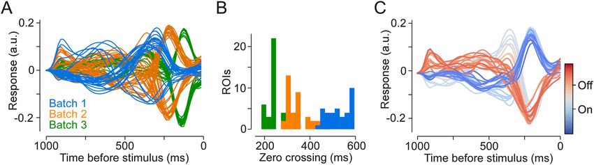
www.nature.com/scientificreports/ www.nature.com/scientificreports
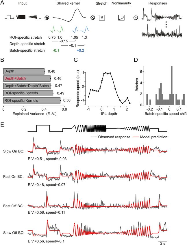
Figure 5. Batch effect estimation using linear models. (A) Design matrix with IPL depth and batch specific
predictors (example scan fields from Fig. 6). (B) Model comparison for On/Off, batch and IPL depth in a linear
model fitted to the local chirp response data (same dataset as in Fig. 4A-E). Error bars indicate 2 S.E.M. (C)
Example traces (grey) for first ROI of each polarity and batch shown in Fig. 6A. Predicted responses from model
using IPL depth alone (red) and with an additional batch specific term (blue). E.V., Explained Variance.
ribbons per type, as reported by Tsukamoto and Omi36. Finally, we estimated the number of ribbons (synapses)
per slice (x-z scan) and BC type by dividing each BC’s axon terminal volume in a slice by its average axon terminal
volume per ribbon (Fig. 4F).
Results
Setting up axial scanning. To allow axial scanning of the retina, we inserted an ETL into the optical path-
way of the 2 P laser of our microscope (Fig. 1). By electrically modulating the optical power of the ETL, the
beam of the 2 P laser entering the microscope´s objective converges or diverges, resulting in a focus shift along
the z-axis of the recording. For the ETL used here, a change in electrical current is transformed into a pressure
change, which in turn regulates the lens volume and, thereby, the curvature of the lens surface (Fig. 1A, inset).
When the lens is positioned vertically (w/optical axis parallel to the table), its fluidic core may be slightly
deformed by gravitational forces, resulting in a deterioration of its optical properties. The simplest horizontal
arrangement would be to place the ETL directly above the objective25,37. However, we decided against this possi-
bility for two reasons: First, in this position, the ETL would introduce a focal plane-dependent change in image
magnification25. Second, if the visual stimulus is coupled into the laser pathway after the scan mirrors – like in our
Scientific Reports | (2020) 10:4399 | https://doi.org/10.1038/s41598-020-60214-z 8www.nature.com/scientificreports/ www.nature.com/scientificreports
Figure 6. Batch effects in axial x-z scans of the mouse inner plexiform layer (IPL). (A) Local chirp responses
from ROIs located in the On sublamina of the IPL. From top: time course of chirp stimulus, heat map showing
glutamate responses of ROIs from three scan fields (batches), average glutamate responses over ROIs in each
batch, and magnified step and frequency responses. (B,C), Local chirp responses of ROIs in (A) projected onto
their first two principal components (PCs), coloured by IPL depth (B) and batch (C).
setup (Fig. 1A)22,30 – the ETL would also modulate the stimulation plane and spectrally filter the stimulus. The
latter is critical if UV stimuli are used: Since prolonged exposure to UV light can degrade the optomechanical
properties of the lens, ETLs are typically equipped with a UV-reflecting glass window (for specifications, see
Table 1). Therefore, placing the ETL into the stimulus path hampers UV stimulation, but UV stimulation is
required to properly drive the mouse retina with its UV-sensitive cone photoreceptors (λPeak = 360 nm; as dis-
cussed in ref. 30). To avoid these issues, we positioned the ETL horizontally in the pathway that reflects the excita-
tion laser onto the scan mirrors (Fig. 1A,B) (F. Voigt, F. Helmchen, personal communication).
To make use of the full aperture of the ETL, we pre-expanded the laser beam using a telescope system (T1).
After the ETL, we used a second telescope system (T2) to refocus the laser beam onto the scanning mirrors. As
T2 determines the beam diameter that enters the back aperture of the objective and the z-range of focus shift
(together with the objective lens’ magnification), it needs to be defined for the specific microscope and the desired
z-range.
First, we evaluated the ETL’s performance using a solution containing the red fluorescent dye SR101 (Fig. 2A).
Our combination of custom ETL driver and optical configuration allowed for a practical focus shifting range of
approx. 200 µm (Methods). Importantly, the same voltage signal reliably resulted in the same z position of the
focal plane (s.d.www.nature.com/scientificreports/ www.nature.com/scientificreports
for large, rapid changes in voltage input – as it happens, for instance, when jumping back from the last line of a
frame to the beginning (retrace) – the ETL´s new refractive state requires a few milliseconds to settle25,29. These
brief oscillations are visible at the bottom of the image (where the frame starts; see particularly Fig. 2D-7). We
dealt with this problem simply by excluding the first couple of lines (~10 ms) of each frame from our analysis.
In addition, we found that the fluorescence smoothly varied along the z axis (Fig. 2C, left scan). The decrease in
fluorescence reflects a loss in laser power, which happens when the ETL changes the beam’s collimation to an
extent that the beam becomes too large for the scan mirrors or is partially blocked by down-stream optics. This
can be improved by applying an offset voltage to the ETL driver signal, such that the laser intensity peak covers
the required z scan range. As the intensity peak is relatively shallow, the IPL of the mouse (~40 µm) can be imaged
with almost constant laser intensity.
Next, we tested whether pixel size and spatial resolution remained constant along the z axis of an x-z scan
suitable for capturing the complete mouse IPL (e.g. 64 × 40 pixels corresponding to 50 × 40 µm). By moving the
microscope’s objective lens, we placed a thin fluorescent film (Methods) at different z positions within an x-z scan
field (Fig. 2D) and measured the film’s thickness. Apart from the artefact (see above), the recorded thickness of
the film remained constant, suggesting that the pixel size is constant along the z axis. Finally, we quantified the
spatial resolution of our system by measuring the point spread function (PSF) of fluorescent beads both in the x-y
plane and at different z positions (Methods). This was done by first setting one of three z planes (Fig. 2E) using
the ETL and then taking image stacks (using the microscope’s motorized stage). The measured PSFs were around
0.4 and 1.8 µm along the x and z axis, respectively, and varied very little for the different ETL planes (Table 3).
In summary, our ETL configuration allows for spatially (nearly) linear, fast axial imaging without detectable
loss in spatial resolution.
Axial scanning in the IPL of the mouse retina. Axial scans were evaluated by imaging light-evoked
glutamate release from BC axon terminals (Fig. 3A). After AAV transduction, the glutamate biosensor iGluS-
nFR26 was ubiquitously expressed across the whole retina, including the IPL (Fig. 3B)7. As the axon terminals of
different BC types stratify at distinct levels of the IPL10,13,38, registering IPL depth within the x-z scans is critical.
Important landmarks in the IPL are the so-called ChAT bands, which are formed by the dendritic plexi of the
cholinergic starburst amacrine cells (SACs)39. Accordingly, a commonly used metrics for IPL depth is to define
the inner (“On”) band as the origin (=0) and the distance to the outer (“Off ”) band as 1 (Fig. 3C) (see also7,34). To
relate these positions to IPL borders, we used transgenic mice in which SACs were fluorescently labelled (Fig. 3B;
for details, see Methods). We found that the relative distance between ChAT bands and IPL borders was highly
consistent across scans and mice (Fig. 3C). Hence, for mice lacking fluorescently labelled ChAT bands, IPL depth
can be reliably estimated from the IPL borders.
The ubiquitous expression of iGluSnFR combined with axial scanning allowed sampling of glutamate release
at all IPL depths (Fig. 4). To achieve scan rates >10 Hz, we used x-z scans with 64 × 56 pixels (1.6 ms/line) at a
zoom factor that yielded a pixel size of ~1 µm (Fig. 4A). Regions of interest (ROIs) were based on local image cor-
relations with an IPL depth-dependent threshold (Methods). This ensured ROI placement across the entire IPL
(Fig. 4B,C). Subsequently, ROIs were quality-filtered using the reliability of their responses7.
To evaluate if the anatomical and functional properties of single ROIs are consistent across x-y and x-z scans,
we compared the distribution of ROI sizes and response quality indices (Supplementary Fig. S1). We found that
ROI sizes were only slightly larger in x-z than x-y scans, which is likely due to the lower resolution in the z- com-
pared to y-dimension (cf. Fig. 2E), but were still within the expected range of BC axon terminals (2–8 µm2, cf.
Extended Data Fig. 1 in ref. 7). In addition, response quality was overall comparable between ROIs recorded in
x-z and x-y scans. The higher number of low-quality ROIs in x-z scans (quality indexwww.nature.com/scientificreports/ www.nature.com/scientificreports
functional diversity that can be recovered from individual x-z scans qualitatively resembles that described in an
earlier study7, reliably capturing signals from BC types with low terminal densities requires integrating data from
multiple scans.
Identification of batch effects. We recorded local chirp light-evoked BC glutamate release from 5,379
ROIs (37 scan fields, 6 mice) across the entire IPL (cf. Fig. 4E). Of those, 3,893 ROIs passed our quality criterion as
previously defined in7 and were selected for further analysis. When visually inspecting the data obtained from dif-
ferent recordings, we noticed that the timing of recorded glutamate traces varied systematically across recordings
(Fig. 6A). We refer to this variation as “batch effects”, in accordance with similar inter-experimental variability in
the single-cell genetics literature (e.g. refs. 43–46).
In our experiments, the variations between scans may have been caused by experimental factors such as slight
temperature fluctuations, as well as differences in light adaptation and/or fluorescence biosensor expression.
To investigate the variability in our data, we performed principal component analysis (PCA) on the recorded
time-series and inspected the projection onto the first two principal components (PCs; Fig. 6B,C). While On
and Off BCs could be distinguished clearly based on the first PC (Fig. 6B), a substantial portion of the variability
observed within On and Off BCs seemed to stem from variability across recordings (Fig. 6C). Qualitatively, these
batch effects were large enough to be a challenge for recovering the biological differences between cell types
within the On and the Off BCs.
We quantified the relative contribution of three factors to the total variance of the observed signal: (1) polarity,
i.e. whether the ROI was located in the On or Off sublamina, (2) IPL depth bin in which the ROI was recorded,
and (3) the batch (scan field) from which the ROI originated. To this end, we fit a series of linear models (Fig. 5A),
each of which included one or more of the three factors (On/Off, IPL depth, batch), and estimated the fraction
of variance explained by the models (Fig. 5B,C). The first model, which captured only the polarity, accounted for
34% of the response variance. The second model, which used only IPL depth as a predictor, accounted for 48%
of the variance. Note that the first model is a special case of the second one, obtained by splitting the IPL into On
and Off sublaminae. As a third model, we used polarity × batch (scan field) ID as a predictor. This model, which
amounts to estimating the average trace of On and Off cells in each scan field, accounted for 66% of the variance,
substantially outperforming the previous models that only considered the biological source of variation. Finally,
adding IPL depth bin as a predictor improved the explained variance only marginally (to 69%).
To summarize, we found that batch effects alone accounted for a larger fraction of the variance than IPL depth
(Fig. 5B), which suggests that accounting for such variation can greatly facilitate any analysis of functional differ-
ences between BC types beyond On vs. Off.
What is the nature of these batch effects? The most salient difference across the three example batches was a
shift in response speed (Fig. 6A). This is especially striking in the response to the chirp’s frequency modulation,
where the batch-averaged responses are almost entirely out of phase (Fig. 6A, bottom right). We found the same
temporal misalignment in the predictions of our model that considered only IPL depth but ignored the batch
effects (Fig. 5C). Comparing the predicted and the recorded traces, we observed that the model was too fast for
the first (slow) batch, approximately aligned for the second (medium) batch and too slow for the third (fast) batch.
This observation is in line with a previous study that reported systematic differences in the response speed of
RGCs recorded from different macaque retinae47.
A possible explanation for shifts in response speed between experiments may be differences in recording tem-
perature. While we used a closed-loop system to keep the temperature of the tissue at 36 °C, small temperature
fluctuations in the order of ±1 °C cannot be excluded. The temperature coefficient (Q10) of biological reactions,
∆T /10
including neural activity, is typically between 2 and 4 (cf. ref. 48), therefore, following Q∆T = Q10 , a tempera-
ture increase of 1 °C may result in a 7 to 15% increase in response speed, which is in the range that we estimated
for the batch effects (cf. Fig. 7D). It is well known that temperature affects neural processing. For instance, sword-
fish actively raise their retinal temperature by 10 to 15 °C, thereby increasing temporal resolution up to ten times
to gain a predatory advantage49.
Building batch and IPL depth variations into a shared BC encoding model. To investigate the
idea that batch effects effectively result in changes in response kinetics more directly, we fit a linear encoding
model and estimated the temporal receptive field kernels of the ROIs in the three example scans shown before.
As expected, the temporal kernels showed systematic differences between the three scans that seem to be largely
explained by rescaling them in time (Fig. 8A,B). Moreover, within a single batch we could still discern the under-
lying IPL gradient: ROIs closer to the IPL centre (=lighter colours in Fig. 8C) had their leading edge closer to zero
and, hence, responded faster. In addition, central ROIs displayed more biphasic kernels and, hence, responded
more transiently.
The data presented above suggest that functional differences between individual ROIs can, to a large extent,
be accounted for by modelling response speed, and this speed depends on two main factors: (1) laminar location
within the IPL and (2) batch effects due to variability between scan fields. We therefore developed a very simple
joint encoding model that reduces the functional differences between neurons (here ROIs) to a temporal rescaling
of their response kernels (Fig. 7A). The model learned exactly one response kernel that is shared among all neu-
rons and all scan fields. In addition, it allowed for a temporal rescaling of this kernel and a neuron-specific scaling
of the response magnitude and polarity-flip (On/Off).
First, we observed that sharing the same kernel shape across all ROIs and only adjusting speed, scale and
polarity yielded a predictive performance of 49% explained variance compared to 56% by the model with an
individual temporal kernel for each ROI (Fig. 7B). While a 7% difference is not negligible, the difference in com-
plexity between the models is considerable: The latter model used more than 40 parameters for each ROI to
specify a response kernel, whereas the former (simplified) model had effectively just 3 parameters to model speed,
Scientific Reports | (2020) 10:4399 | https://doi.org/10.1038/s41598-020-60214-z 11www.nature.com/scientificreports/ www.nature.com/scientificreports
Figure 7. Encoding model comparison. (A) Model design: the input time series of the chirp stimulus is
convolved with a finite impulse response linear filter which is sign-flipped for On and Off responses and
stretched by a factor that is learned for each ROI, then passed through a static nonlinearity (exponential
linear unit) and weighted by each ROI to produce the predicted trace. (B) Comparison of the different speed
models (Methods) learned simultaneously with the encoding model. Error bars indicate 2 S.E.M. (C) Speed as
a function of IPL depth. (D) Distribution over learned batch shifts. (E) Observed (black) and predicted (red)
traces for four ROIs. E.V., Explained Variance.
scale and polarity for each ROI. Moreover, the simplified model allows us to assess how well we can predict the
response speed of individual ROIs based on their IPL depth and a batch-specific speed adjustment. The complex
model – while more accurate – does not allow us to make such abstraction, because it models each ROI separately
Scientific Reports | (2020) 10:4399 | https://doi.org/10.1038/s41598-020-60214-z 12www.nature.com/scientificreports/ www.nature.com/scientificreports
Figure 8. Differences in response speed between batches. (A) Learned temporal kernels for all ROIs with E.V.
> 0.5. Coloured by batch (same batches as in Fig. 5). (B) Zero crossings (after first peak) for all ROIs with E.V. >
0.3. (C) All ROIs of the 2nd batch (orange in A,B) with E.V. > 0.3, coloured by IPL depth.
and does not include any simplifying assumption of shared variability between ROIs. For us, it serves as a bench-
mark to judge the interneural variability in the shape of the response kernel, which the simpler model cannot
capture by design. Therefore, for the remainder of the paper, we focussed on the simplified model.
Next, we tested the effect of additionally constraining this simple model: First, we assumed that the speed of
each ROI is only a function of the ROI’s depth in the IPL. This assumption, which meant that all ROIs with the
same laminar location share the same response kernel, decreased the predictive performance to 40% explained
variance (Fig. 7B). Alternatively, allowing for batch effects by adding a scan field-specific global shift to the speed
estimates for all the ROIs in the same scan field, enabled us to capture 46% explained variance. This was similar
to the model that allowed each ROI its own speed (49%). Additionally, including an interaction term between
IPL depth and batch improved performances only slightly (47%), suggesting that batch variations had similar,
approximately additive effects onto the speed across the IPL.
In summary, to the extent that variability between BCs can be modelled by differences in response speed,
these speed differences can almost entirely be accounted for (46% vs. 49% explained variance) by laminar location
within the IPL and a batch-specific global shift in response speed.
Moreover, with this model we can give a quantitative estimate of the speed gradient across the IPL (Fig. 7C).
In line with earlier reports7,15,20,21, the BC response speed fell off from the centre of the IPL towards its borders.
Notably, between the ChAT bands this speed gradient was nearly symmetrical between On and Off BCs. However,
after that the On BCs levelled off and exhibited the same, relatively slow speed until the ganglion cell layer. The Off
BCs, by contrast, continued decreasing in their speed almost all the way until the inner nuclear layer.
Discussion
We implemented fast axial x-z scanning of the whole-mounted mouse retina by equipping a 2 P microscope24 with
an ETL to rapidly shift the focal plane of the laser. We showed that this experimental setup is suitable to record
the light-evoked glutamatergic output of BCs almost simultaneously across the complete IPL. Axial scans enabled
comparing temporal response properties between IPL strata more directly than “traditional”, time-consuming
series of horizontal (x-y) scans. At the same time, x-z scans allowed identifying batch effects, characterized mostly
by inter-experimental differences in signal speed. We showed that already batch correction with a simple linear
model can improve recovering the characteristic response speed profile across the IPL. Our results indicate that
careful consideration of inter-experimental variance is key for extracting functional differences between neurons.
Techniques for axial scanning. Several technical solutions that enable fast axial scanning in 2 P micros-
copy have been published. Here, two main approaches can be distinguished:
In the first group, a focus change within the sample is realized by moving the objective lens relative to the sam-
ple (or vice versa). This has, for instance, been implemented using a piezo to move the objective along the z axis50.
By coordinating the trajectories of galvo scanners (x-y) and piezo (z), fast volume scanning (i.e. 10 Hz frame rate
for a 0.25 mm cube) can be achieved using 3D spiral patterns. While this solution is relatively easy to implement,
the inertia of the objective limits the speed with which a focal plane can be selected. In addition, the objective’s
movements may introduce vibrations to the sample.
In the second group, focus shifting is achieved by changing the collimation of the laser beam (“remote focus-
sing”) while the objective-to-sample distance remains constant. This strategy eliminates movements close to the
sample. A classical solution for remote focussing is to add a reference objective to the laser path to axially displace
the focal plane in the sample51. Because only a lightweight mirror under this reference objective is moved, this
arrangement can reach high axial velocities. However, its superb optical performance is offset by high complexity
(i.e. optical alignment; ref. 52) and the costs of a second high-quality objective. In a different approach, an arrange-
ment of inertia-free acousto-optical deflectors (AODs) replaces the galvo scanner and, thus, allows for very fast
random-access scanning25,53–56. Using a clever AOD arrangement, random-access in 3D is possible54,57. Due to
the absence of mechanical parts, such a solution enables extremely fast focus changes (1 mm). However, AOD-based solutions typically are complex and expensive systems, which usually require
substantially more laser power than galvo scanner-based systems.
Comparably fast remote focussing can also be achieved with an ETL, in which the curvature – and
hence the focal length – of a liquid lens core is controlled electrically (reviewed in ref. 58). With high-quality
Scientific Reports | (2020) 10:4399 | https://doi.org/10.1038/s41598-020-60214-z 13www.nature.com/scientificreports/ www.nature.com/scientificreports
inexpensive ETLs becoming available, they offer a cost-efficient and relatively simple way for equipping mechan-
ical scanner-based (or “simple” 2D AOD-based) fluorescent microscopes, including confocal59, 2P25,37,60,61, and
light-sheet systems29,62, with fast focussing. In the simplest configuration, the ETL is positioned directly on top of
the objective lens25,37. However, in this position, shifts in focal plane are accompanied by image scaling in x-y25.
Also, the ETL’s transmission in the relevant spectral bands – like here, the UV transmission for light stimulation
(cf. Results) – may need to be considered. By integrating the ETL into the laser path upstream of the scan mir-
rors59, image scaling and (potential) ETL transmission issues are avoided. The additional telescope needed to
couple the ETL into the laser path slightly increases complexity but at the same time allows adapting the available
z range to the experimental needs.
In the current study, we applied ETL-enabled axial scanning to the isolated but intact whole-mounted mouse
retina. We found axial scans to work across the whole mouse retina63 – except for areas very close to the optic
disc (where the nerve fibre layer becomes very dense) or close to the edge (damage from excising the retina). Our
approach should in principle be applicable to a wide range of experiments, including in vivo recordings in the
brain. As with other optical techniques, a main limitation of scanning depth is scattering within the tissue.
Further improving ETL-based axial scanning in the ex-vivo retina. For x-z scans across the mouse
IPL, we used a unidirectional scan mode, where at the end of a frame, the focal position of the excitation laser
is shifted back to the first scan line in one ~50 µm “jump”. This results in the aforementioned artefact in the first
few lines of each frame and is caused by fast oscillations in the ETL’s focal power after a rapid change in driving
current (see link to specifications, Table 1). The stabilization time of ~10 ms (for travel distances of ~50 µm) we
observed is consistent with earlier reports25,64. For simplicity, we here used scans with more lines, such that the
artefact was outside the IPL. Alternatively, optimizing the current trajectory driving the ETL – e.g. by using a
steep ramp and “overdriving” the current instead of just a step (cf. ref. 25) – may dampen the ETL’s oscillations and,
thus, decrease settling time. Also, bidirectional scans that do not require large and rapid changes in z position may
reduce such z travel distance-dependent artefacts.
Another potential caveat of an ETL is thermal drift, because driving the lens may slowly heat it up. Since
the resistance of the coil that shapes the lens’ core is temperature-dependent, also the current-to-focal power
relationship depends on the ETL’s temperature (for details, see ETL specs). We embedded our ETL into a solid
adapter ring made from aluminium, which seemed to have kept the ETL’s temperature stable enough, as we did
not observe any relevant thermal drifts during the course of a recording. In any case, the ETL model we used
features a build-in temperature sensor that can be read out via an I²C (Inter-Integrated Circuit) bus connection
to monitor the ETL’s temperature.
One consequence of the ETL being positioned upstream of the scan mirrors is a focus dependent change in
laser power. Because we needed a relatively small z focus range to scan across the mouse IPL, we applied an offset
voltage to the ETL, shifting the shallow peak in laser power to the imaging range. For larger z ranges, one could
automatically adjust the laser power with a sufficiently fast modulator (i.e. a Pockels cell) as a function of the ETL’s
control signal.
Identification and removal of batch effects in axial scans of the mouse IPL. Batch effects – refer-
ring to inter-experimental variability – recently became a prominent topic in the single-cell genetics community
(e.g. refs. 43–46), which motivated us to look for such effects in our data. Note that the batch effects we observed in
the presented data are not specific to axial scans (or optical recordings). Instead, batch effects reflect experimental
variability that can result from small differences in recording conditions (i.e. temperature; see below) but also
method-specific variations: For imaging, this could be labelling intensity; for electrical single-cell recordings,
electrode tip geometry.
For the functional characterization of retinal cell types, our previous studies used data obtained from sequen-
tial x-y recordings7,28. In the IPL, one disadvantage of this approach is that the sample of BC types in each indi-
vidual scan greatly varies between scans, and the cells recorded within any one scan will typically share similar
response properties. In the middle of the IPL, a third of all BC types can theoretically be recorded in an individual
x-y plane (see stratification profiles in refs. 10,13,38), but typical scans will mostly sample 2 or 3 BC types. In con-
trast, axial x-z scans established here allow less biased recordings of the glutamate output across the entire IPL,
with BC types with very different response properties present in the same scan field. As a result, each scan exhib-
ited a highly stereotypic functional organization of response kinetics across the IPL, as described before7,15,20,21.
This property greatly facilitated comparison of data obtained by different recordings, which allowed us to detect,
quantify and correct for batch-specific variability in BC responses (see below).
In our recent studies characterizing BC and RGC types7,28, we did not explicitly correct for batch effects.
However, we used other measures to minimize the effect of such inter-experimental variations on clustering. For
BC recordings, we estimated a prior probability for cluster allocation for each scan field taken at a specific IPL
depth, which was based on the relative axon terminal volume of all BC types at the respective depth (cf. Figure 2c
in ref. 7). This is similar to clustering separately within bins of IPL depth, which helps to identify – on average –
BC type-specific response signatures. The fact that ROIs from single scan fields were consistently assigned to dif-
ferent functional types suggests that type-specific differences could be resolved despite the variability induced by
batch effects. For GCL recordings, we judged response quality based on alpha RGCs65, which are easily recognized
by their large somata. Only if alpha RGCs displayed their characteristic temporal response profile65,66, we included
the data. By doing so, we implicitly minimized the variability induced by batch effects. Again, we found that most
functional groups were present across experiments, suggesting that experiment-specific speed differences did not
induce additional functional clusters. Thus, if a readily identified and well-calibrated reference exists, batch effects
can be reduced by excluding recordings that deviate strongly. However, this approach can only reduce batch
Scientific Reports | (2020) 10:4399 | https://doi.org/10.1038/s41598-020-60214-z 14You can also read