Simulation of the COVID-19 pandemic on the social network of Slovenia: estimating the intrinsic forecast uncertainty
←
→
Page content transcription
If your browser does not render page correctly, please read the page content below
Simulation of the COVID-19 pandemic on the social network
                                              of Slovenia: estimating the intrinsic forecast uncertainty
                                                                  Žiga Zaplotnik, Aleksandar Gavrič, Luka Medic
                                                                                         May 28, 2020
arXiv:2005.13282v1 [q-bio.PE] 27 May 2020

                                                                                            Abstract
                                                      In the article a virus transmission model is constructed on a simplified social network.
                                                  The social network consists of more than 2 million nodes, each representing an inhabitant
                                                  of Slovenia. The nodes are organised and interconnected according to the real household
                                                  and elderly-care center distribution, while their connections outside these clusters are semi-
                                                  randomly distributed and fully-linked. The virus spread model is coupled to the disease
                                                  progression model. The ensemble approach with the perturbed transmission and disease
                                                  parameters is used to quantify the ensemble spread, a proxy for the forecast uncertainty.
                                                      The presented ongoing forecasts of COVID-19 epidemic in Slovenia are compared with the
                                                  collected Slovenian data. Results show that infection is currently twice more likely to transmit
                                                  within households/elderly care centers than outside them. We use an ensemble of simulations
                                                  (N = 1000) to inversely obtain posterior distributions of model parameters and to estimate
                                                  the COVID-19 forecast uncertainty. We found that in the uncontrolled epidemic, the intrinsic
                                                  uncertainty mostly originates from the uncertainty of the virus biology, i.e. its reproductive
                                                  number. In the controlled epidemic with low ratio of infected population, the randomness
                                                  of the social network becomes the major source of forecast uncertainty, particularly for the
                                                  short-range forecasts. Social-network-based models are thus essential for improving epidemics
                                                  forecasting.

                                            1    Introduction
                                            The ongoing COVID-19 epidemic has revealed a major gap in our ability to forecast the evolution
                                            of the epidemic. There are several ways to simulate the epidemic dynamics. The most common
                                            approach is using compartmental models of susceptible (S), immune (I), recovered (R) population,
                                            i.e. SIR models [1, 2]. These are described by a system of differential equations given some
                                            predefined parameters, such as probability of the disease transmission and the rate of recovery
                                            or mortality. Another variation of the SIR model is a SEIR model, which accounts also for the
                                            exposed (E) population, representing infected but not yet infectious subjects. The SEIR model
                                            is combined with activation functions to smoothly model social factors affecting virus spread and
                                            the disease progression. A major setback of the deterministic epidemic models is that they are
                                            only applicable for sufficiently large populations, where the assumption of homogeneous spread of
                                            the virus is valid [3]. For coronaviruses, there is evidence that some infectious cases, the so called
                                            superspreaders, spread virus more than others [4]. Their role is of the utmost importance in the
                                            initial uncontrolled phase of an epidemic and in its final controlled phase with low population
                                            of infected. Thus, deterministic SEIR models are also unable to properly describe the intrinsic
                                            uncertainty of the virus spread due to heterogeneous connectivity of the social network and due
                                            to heterogeneous disease progress of the infected population.
                                                Consequently, we use node-based approach [5] to simulate the SARS-CoV-2 coronavirus spread
                                            over a simplified social network of more than 2 million nodes with a total of up to 20 million
                                            connections, representing the population of Slovenia and the connections of its inhabitants, with
                                            realistic distinction between household and outer connections. Despite being computationally more
                                            expensive, an advantage of network approach is that it allows direct simulation of intervention

                                                                                                 1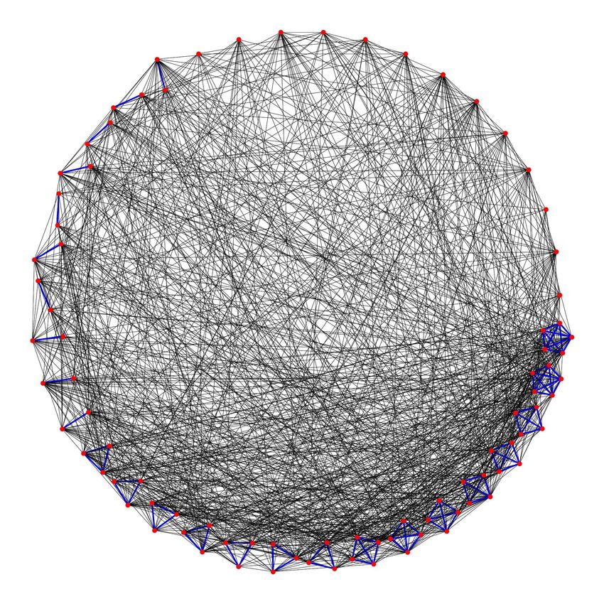
k persons in household     number of k-person households
                  1                          269898
                  2                          209573
                  3                          152959
                  4                          122195
                  5                          43327
                  6                          17398
                  7                          6073
                  8                          3195
                  25                         100 care centers with 8 groups each

Table 1: Households distribution in Slovenia, based on the data of Statistical Office of Republic
of Slovenia [7].

measures as well as planning of the future strategies of the the virus containment [e.g. 6] and
lockdown-exit strategy. Here, we combine the network approach together with an ensemble-of-
simulations approach which allows to estimate the uncertainty of the predictions which stems
from the randomized network, initial number of infected, and the uncertainty of the coronavirus
transmission parameters and disease progress parameters.
    Section 2 describes the social network model, the virus transmission model and the coupled
disease progression model. The probabilistic ensemble forecast of the COVID-19 pandemic for
Slovenia and the contribution of different model components to the total forecast uncertainty is
described in Section 3. Discussion, conlusions and further outlook are given in Section 4.

2     Methodology
2.1    Social network model
The social network model of the population of Slovenia distinguishes household connections and
connections outside households. A total of N = 2045795 nodes is used in the social network.
The number of k-person households is given in Table 1. There are approximately 100 elderly
care centers in Slovenia with a total of approximately 20000 residents. Each elderly care center is
assumed to include 8 distinct groups of 25 people. Average household/care group consists of 2.5
people in Slovenia so the average number of contacts per person within household is 1.5.
    In normal conditions, contact number distribution follows power law with fat tails [8], which
are associated with superspreader events, e.g. large public gatherings such as sport and cultural
events. However, since all public events are canceled in the event of the COVID-19 epidemic, these
fat tails are cut off [9] and the topology of the social network changes substantially. In conditions
without large public gatherings, it is reasonable to assume that certain people still have much
larger number of contacts than others. The studies of social mixing, e.g. POLYMOD study of
social interactions within 8 European countries, typically report negative binomial distribution
of the number of contacts [10, 11]. We assumed mean number of contacts outside households to
be 13.5 with standard deviation of 10.5. Instead of negative binomial distribution, we rather use
smooth gamma distribution, which resembles the shape of the binomial distribution but has some
useful mathematical properties, which will be exploited in the continuation. Thus, we model the
connectivity, i.e. the number of contacts per person, using the gamma probability distribution,
which is essentially an exponential distribution
                                                    1             x
                                   p(x; k, θ) =         k
                                                          xk−1 e− θ .                            (1)
                                                  Γ(k)θ

In this study, we use k = 1.65 and θ = 4.08 for the initial setup, which gives an average number of
13.5 contacts per person per day (Fig. 1). Together with 1.5 family contacts per person per day,

                                                   2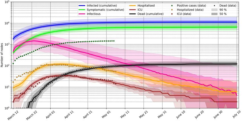
Figure 1: Number distribution N (x) = p(x)N by the number of contacts in the social network
model. The black graph shows the assumed distribution of people with a given number of outer
contacts in a normal, non-epidemic, phase, while the red graph presents reduced number of outer
contacts in the case of a social distancing measures.
the total number of contacts per person per day is 15. Here, we assume that the average number of
contacts is the same for each age group, despite studies showing that elderly have reduced number
of contacts [12]. The average contact number per person per day varies for different countries [11],
however 15 contacts per day is a reasonable guess for Slovenia. We also assume quasi-static social
network, i.e. only 20% of contacts are new every day, and the remaining 80% are static. This
choice is a first guess, justified by the fact that only around 20% of all daily contacts last less than
15 minutes [11]. These can be regarded as random sporadic contacts. Self-distancing measures to
mitigate COVID-19 can be imposed by decreasing parameter θ, which also decreases the average
number of outer contacts (Fig. 1).
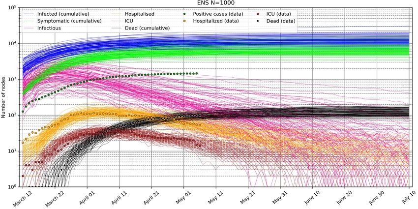
Fig. 2 shows an example of the connectivity change of a minimised network with 88 nodes
clustered on a circle with the real household distribution taken into account.
Technically, we connect the graph in the following way:
1. number of outer contacts for each node is randomly drawn from Gamma distribution (1). If
node i has xi = 0.33 contacts per day, it means that it will have 0 contacts 2/3 of the time
and 1 contact 1/3 of the time of the simulation;
2. for each node i, we randomly assign the connections to xi other nodes, where xi is the number
of contacts of node i. However, not every node has the same probability of being picked
as a neighbour. Node j, which has xj contacts, is picked as a neighbour with probability
xj N (xj )/T , where N (xj ) is the number of nodes with xj contacts and T is the total number
of contacts in the network (T is twofold the number of connections). Sampling over Gamma
distribution (1) gives us a distribution of N (x) = p(x)N . When picking the neighbours, we
actually sample the same Gamma distribution times x, i.e.
1 x
pn (x) = p(x; k, θ)x = k
xk e− θ ∝ p(x; k + 1, θ). (2)
Γ(k)θ
3. The shape of the social network is changing (80% of connections static, 20% changing) at
every timestep of the simulation to account for random sporadic contacts. (a) The number
of contacts of node i is fixed (randomly jumps between bxi c and dxi e based on the value of
xi ). For example, if a node has 0.33 contacts per day, 1 contact is picked with probability
3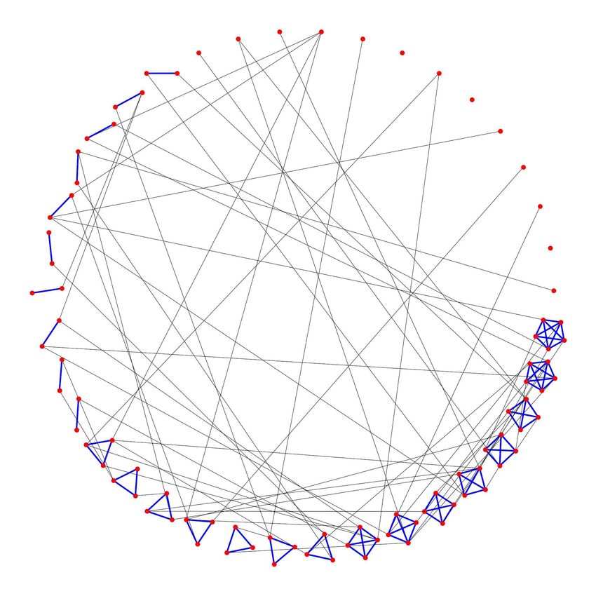
a)                                                     b)

Figure 2: Connectivity of the social network of N = 88 nodes for a) densely connected graph,
where each node has on average 15 contacts per day (1.5 family and 13.5 outer contacts, θ = 22.5)
and b) sparsely connected graph, where each node has on average 2.5 contacts per day (1.5 family
and 1 outer contact). Red dots are nodes, blue lines represents household connections and black
lines outer connections. The graph represents a minimized version of the social network used in
the virus spread simulation.

        1/3 and 0 contacts with probability 2/3. (b) The social network is partially rewired at every
        timestep to account for superspreaders mobility.
    An important advantage of our network approach is that the nodes are not connected randomly
through “half-links” (directed connections linking egos to their contacts, the alters) [13, 14], such as
in the vast majority of modelling studies, where the WAIFW (who-acquires-infection-from-whom)
matrices were constructed based on the egocentric data. Instead, nodes are fully-linked.

2.1.1     Compartments
Similarly as in the deterministic SEIR model, we divided the population into compartments,
where we used the following compartmental division: susceptible, infected, infectious (exposed),
hospitalised with severe illness, hospitalised and critically ill (ICU treatment), hospitalised and
fatal, and recovered. The latter are assumed to be immune for the whole simulation period. In the
network model, a susceptible node becomes exposed (infected) with a certain probability (called an
attack rate) when in contact with an infectious node. After a certain period of time, the infected
node progresses into infectious state. In the accordance with the chosen compartmental division
we monitor each node by adapting its clinical state at every timestep. Since all the periods are
stohastic variables, e.g. infectious and recovery periods, those periods widely vary among the nodes
(and the variations would be even greater if we would account for the demographic properties,
e.g. age and sex).

2.2      Virus transmission model
2.2.1     Reproduction number R0
A basic reproduction number, R0 , provides information on the average speed of virus transmission
in an uncontrolled phase of the epidemic. Different methodologies produced different results,

                                                   4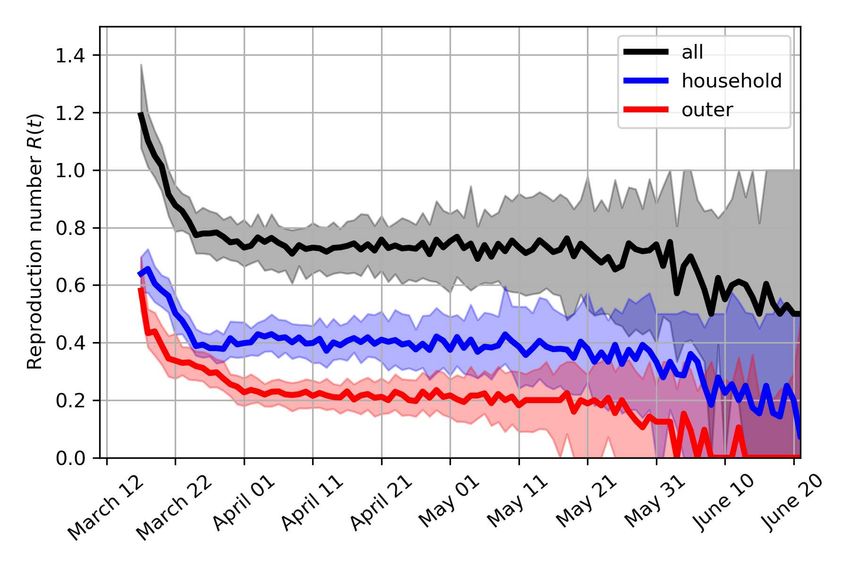
however the majority of reported R0 for SARS-CoV-2 is within 2 and 3. Here, we use median
reported R0 from a number of studies, as well as its median confidence intervals, i.e. R0 = 2.68,
with 95% confidence interval [2, 3.9]. This approach is not the optimal one, since we are trading
accuracy for precision. The published R0 values as well as our deduced R0 distribution is shown
in Fig. 3a,b. The optimal log-normal distribution should thus match the following conditions:
CDF(R0L ; µ, σ, ∆x) = 0.025, CDF(R0U ; µ, σ, ∆x) = 0.975, and median(CDF) = R0 , where R0L and
R0H are lower and upper boundaries of R0 , CDF stands for log-normal cumulative distribution
function and its median is exp(µ). Then, we define a quadratic cost function, which includes
all the above criteria, and by minimizing it, we obtain the optimal parameters for log-normal
distribution: ∆x = 0.36, σ = 1.14, exp µ = 1.54.

 a)                                                  b)

                          c)

Figure 3: a) Basic reproduction number R0 (median and 95% confidence interval), reported in a
number of studies for different locations [15, 16, 17, 18, 19, 20, 21, 22, 23, 24, 25] and references
therein. b) Log-normal probability density function of the basic reproduction number, used for
ensemble simulations. c) Probability distribution of secondary attack rates for household contacts
and outer contacts.

2.2.2   Attack rate
In general, the basic reproduction number, R0 can be decomposed into the secondary attack rate
times the number of contacts. The secondary attack rate (SAR) is defined as the probability
that an infection occurs among susceptible people within a specific group (i.e. household contacts
or other contacts outside households). The measure can provide an indication of how social
interactions relate to the transmission risk. We can further decompose the R0 into the household
risk of infection and outer risk of infection (following [26])

                                    R0 = SARh Nh + SARc Nc ,                                     (3)

                                                 5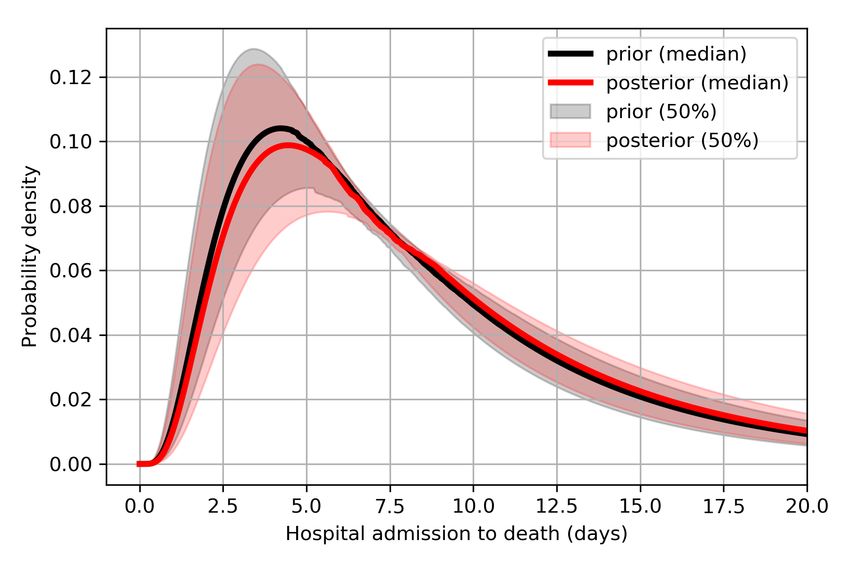
where SARh and SARc are secondary attack rates within household and outside household (outer
contacts), respectively. Nh and Nc are the numbers of household contacs and outer contacts.
Here, one must notice that the above estimation of SARh assumed homogeneous mixing, while
the network model is heterogeneous with R0 = SARh (hNh i + Var(Nh )/ hNh i) + SARc (hNc i +
Var(Nc )/ hNc i). To be consistent with Liu et al. [26], we stick with formulation (3).
    The study of Liu et al. [26] suggest SARh value of 35% (95% CI 27-44%) for SARS-CoV-2.
SARh is almost normally distributed with mean 35% and 2σ ≈ 8.5. The distribution of R0 is
given in the previous paragraph. It holds: SARc = (R0 − SARh Nh )/Nc . This gives a transmis-
sion efficiency of SARc = 16% (95% CI 10.8-25.1%). Fig. 3c shows probability distributions of
secondary attack rates as used in the ensemble of simulations.
    If the social infectious period is Tinf ≈ 5 days (check subsection 2.3.4), we can assume that
the daily risk of getting infected from a certain household member is SARh,daily where 1 − (1 −
SARh,daily )Tinf = SARh and

                                                       ln (1 − SARh )
                               SARh,daily = 1 − exp                                           (4)
                                                             Tinf

being equal 8.3% (95% CI 6.1-10.9%). Similarly, we compute SARc,daily = 3.4% (95% CI 2.3-
5.6%).
   Some studies [e.g. 27] have concentrated only on the symptomatic secondary attack rates and
have shown relatively smaller numbers: 0.45% (CI=0.12%-1.6%) among all close contacts and
10.5% (CI=0.12%-1.6%) among household members. However, these numbers cannot reproduce
the reported R0 between 2 and 3.9 with any realistic number of contacts. Another study shows
similar attack rates to what we use here [28].
   The attack rate affects the virus transmission as follows. At each timestep of the simulation
(every 1 day), the susceptible contacts of each infectious individual are randomly infected with
probability SARh,daily or SARc,daily , depending whether the contact occurs within household or
outside it.

2.3     Disease progression model
A simplified sketch of the disease progression model is shown in Fig. 4a. When a certain individual
(node) gets infected, incubation period starts and several days will pass until the symptom onset.
The majority of the infected people recovers at home, some die at home, while certain individuals
are admitted to hospital in the following days. Several outcomes are possible: recovery after
normal hospitalisation, recovery after intensive care unit hospitalisation and death. Note that for
every node, the illness evolves differently based on the probability distribution described in the
following subsections.

2.3.1   Case fatality ratio
The baseline case fatality ratio (CFR), i.e. the fatality ratio among all positively tested, is assumed
1.38% (CI 1.23-1.53%) [29, 32], similar to the estimate of Shim et al. [33] for South Korea. Dividing
deaths-to-date by cases-to-date leads to a biased estimate of CFR, called naive CFR (nCFR) as
the delays from confirmation of a case to death is not accounted for, as well as due to under-
reporting of cases and even deaths. The reported numbers agree with recently published study
for symptomatic case fatality ratio in China [34].

2.3.2   Infection fatality, intensive care and hospitalisation ratios
Infection fatality ratio (IFR) estimates are based on the study from Verity et al. [29], which
reported IFR of 0.66% with 95% confidence interval 0.4% to 1.3%. These estimates are consistent
with IFR on Princess Diamond Cruise ship, when demographic differences are accounted for [35].
In Imperial College report on COVID-19 [36], these numbers have been also adjusted for the non-
uniform attack rate and UK demography. The authors obtained age-stratified IFR estimates by

                                                  6
Incubation
period
Infectious
period
Illness onset to
hospitalisation
Hospitalisation
severe cases
Hospitalisation
critical cases
Hospitalisation
to death
Home
recovery
Home
death
c) d)
Figure 4: a) A simplified sketch of illness evolution. b) Infection fatality ratio distribution and
infection hospitalisation ratio distribution for ensemble simulations. Computed based on data
from Verity et al. [29]. c) Incubation period and illness onset to hospitalisation distribution for
COVID-19 patients [30]. d) Mean distribution of hospital admission to death, hospital admission
to hospital leave for severe and for non-severe illness [30, 31].
7adjusting their CFR estimates using COVID-19 prevalence data for expatriates evacuated from
Wuhan. This approach involves very large uncertainties. Furthermore, Verity et al. [29] collected
data from patients who were hospitalised in Hubei, mainland China, where median age is 37.4
years while median age in Slovenia is 44.5 years. Study reported a strong age gradient in risk of
death. We have applied those age-stratified estimates to the Slovenian population. Performing
an age-stratified weighted average, we compute the total IFR of 1.16% (CI 0.63-2.22%). Similar
total IFR was reported by a comprehensive study for Italy [37] (1.29%, 95% CI 0.89-2.01%). On
the other hand Modi et al. [38] have recently estimated somewhat lower IFR (0.95%, 95% CI
0.47-1.70%) with the lower bound of 0.65% for Lombardia, consistent with 0.58% lower bound for
Bergamo province. Villa et al. [39] reported a bit higher IFR of 1.6% (95% CI 1.1-2.1%). A more
comprehensive meta-analysis of IFR estimates was done by Meyerowitz-Katz and Merone [40].
Analogously, we compute the average hospitalisation rate of 6.37% (95% CI 3.8-13%) based on
Verity et al. [29]. Slightly lower age-dependent hospitalisation rates were estimated for COVID-19
patients in USA by Garg et al. [41], which adjusted for demography of Slovenia (but not accounting
for non-uniform attack rate) gives hospitalisation rate of 3.97%. The latter result better coincides
with the observed number of hospitalisations in Slovenia. No interval estimate is given, thus we
use the same relative error as given by Verity et al. [29]. The final hospitalisation rate is thus
3.97% (95% CI 2.37-8.10%). We assume that roughly 1/4-1/3 of all hospitalised cases are admitted
to ICU [42], despite some studies showing smaller proportions [43]. We assume that one half of
cases admitted to intensive care unit (ICU) are fatal [44].
Taking into account infection fatality ratio, hospitalisation ratio and ICU admission ratio, it
follows that roughly one half of all deaths occur at home/elderly care center/palliative care center,
which agrees with the present data for Slovenia [45]. Note that for simplicity, we have assumed
uniform attack rate across all ages, despite studies showing that working population is most likely
to get infected [46, 47]. Using the minimization procedures, we obtain parameters of log-normal
distribution which best fits both values and their 95% confidence interval (Fig. 4b).
2.3.3 Incubation period - infection to illness onset
Mean incubation period is taken to be 5.0 days (95% CI 4.2-6.0 days), while the 95th percentile
of the distribution was 10.6 days (95% CI 8.5-14.1 days) and 99th percentile 15.4 days (99% CI
11.7-22.5 days) [30]. Similar numbers were reported in earlier studies with less patients included
[19, 48, 49, 50]. Log-normal distribution is used among for incubation period among nodes.
However, the parameters of the lognormal distribution remain fixed due to numerical instability
of their computation. Thus, all ensemble members have the same log-normal distribution of
incubation period. Incubation period distribution and other outcome parameters are shown in
Fig. 4c.
2.3.4 Infectious period
The infectious period is not yet well defined. A small study from German cohort of only 9
patients with mild clinical courses [51] showed that viral shedding was high during the first week
of symptoms and peaking at day 4. Another study from Singapore reported seven clusters in
which virus was transmitted from a COVID-19 patient before experiencing symptoms. According
to the authors pre-symptomatic transmission occurred 1-3 days before symptoms onset [52]. We
have therefore estimated latent (non-infectious) period of 3 days and infectious period to start
2 days before the completion of incubation period (average incubation period is estimated at 5
days). Thus, we assume 2 days of pre-symptomatic transmission. Slightly larger numbers (2.55
days for Singapore and 2.89 days for Tianjin, China) were reported by Tindale et al. [53].
The infectious period likely ends around 5 days from symptoms onset, so the total period of
infectiousness lasts Tbioinf ≈ 7 days. Note however that none of the interval boundaries are known
exactly. Determining its final boundary is especially challenging, as it depends on the social factors
as well, e.g. whether the infected cases are able to self-isolate from surroundings and how strictly
they follow the self-isolation order. Here, we assume strict (100%) self-isolation and use a social
8infectious period of Tsocinf = 5 days. It starts 2.5 days (95% CI 1.5-3.5 days) after infection and
end 2.5 days after incubation (95% CI 1.5-3.5 days) as the case ascertainment typically occurs 2
days after symptoms onset [54]. The infectious period fall in line with study of Bi et al. [28], Fig.
S2. It also falls in line with the reported proportion of pre-symptomatic transmission (representing
half of infectious period) being 48% for Singapore, 62% for Tianjin, China [55] and 44% for 77
infector-infectee pairs in Gaungzhou, China [56].
2.4 Illness onset to hospitalisation or home recovery
From the illness onset on, there are two possible recovery pathways: home recovery or hospitali-
sation (Fig. 4c). Home recovery period for mild cases has not been documented officially but is
reported to be within one and two weeks. Since it does not affect the hospitalisation statistics, we
here assume it to be log-normally distributed with mean period of 10 days.
Based on the clinical study of Linton et al. [30], mean illness onset to hospital admission period
is 3.9 days (95% CI 2.9-5.3 days), with median of 1.5 days (95% CI 1.2-1.9 days), 5% percentile
at 0.2 days (95% CI 0.1-0.3 days) and 95% percentile at 14 days (95% CI 10.3-20.1 days). Only
the distribution of data for living patients is accounted for, since we now understand the severity
of the illness. In China, fatal cases were admitted to hospital on average two days later [30].
2.5 Hospital admission to recovery or death
Hospital admission to death median (mean) length is assumed 6.7 (8.6) days long (Fig. 4d). Only
slightly longer periods were reported by Mizumoto and Chowell [57] with mean length of 10.1 days.
Hospital admission to recovery is on average longer than hospital admission to death. The median
hospitalisation length is 11 days (95% CI 10-13) for non-severe cases and 13 days for severe (95%
CI 11-17) [30]. Both are log-normally distributed. For ensemble computations, their medians
are further log-normally distributed according to their respective confidence intervals. Similar
numbers were reported by Zhou et al. [58] with 11 day (95% CI 7-14) mean hospital length of stay
and 8 day (95% CI 4-12) mean ICU length of stay.
Fatality ratio of severe cases in need of intensive care is reported to be around 50%. We assume
fatality ratio of severe cases without intensive care to be normally distributed with mean of 90%
(95% CI 85-95%). Fatality ratio of severely ill without oxygen is assumed 10% (95% CI 5-15%).
2.6 Initial condition
The initial condition for the simulation is defined for March 12, 2020. To that day, there were 131
symptomatic cases who tested positive in Slovenia, 8 days after first positive case, which implies
an anomalously low doubling time of τ = 1.23 days. This number is case specific as there was
winter holiday in Slovenia at the end of February and beginning of March. Thus, lots of cases were
imported from Northern Italy (including Lombardy). Other studies typically suggest a doubling
time of around 5 days (95% CI 4.3 - 6.2) in the initial uncontrolled stage of the epidemic [59].
However, Abbott et al. [60] report smaller values of around 3.5 days in most of Western Europe.
Thus, our choice is doubling time of Tdouble = 3.5 days (95% CI 2.5-4.5 days) for the period before
March 12.
Different numbers of actually infected people were suggested in the media reports, ranging
from 5 to 20 times the number of reported positive cases. Given the average incubation period
Tinc +2
of 5 days + (2 days for case ascertainment) and doubling period of 3.5 days, factor 2 Tdouble = 4
applies. Furthermore, the proportion of asymptomatic cases is around 18% based on the data
from Diamond Princess Cruise Ship [61] (mostly older people) and around 33% based on the
more recent study [62]. Population screening tests from Iceland reported 41.6% of all who tested
positive, did not experience any COVID-19 symptoms [63]. Similar asymptomatic ratio (43.2%
(95% CI 32.2-54.7%)) was reported also from a screening study conducted for the Italian town
Vo [64]. Another study on the homeless population in Boston reported even larger proportion of
9Figure 5: Distribution of 1780 infected people on March 12, 2020, in Slovenia, by the duration of
their infection.
asymptomatic cases [65]. The model-driven study of Emery et al. [66] found that 74% (95% CI 70-
78%) of SARS-CoV-2 infections proceeded asymptomatically, raising also doubts about the IFR.
In this study, we opt for 40%, normally distributed with standard deviation of 10%. Furthermore,
we double the value to account for the initial under-reporting of symptomatic cases, estimated
by Kucharski et al. [17]. All together, this results in almost 1800 infected people in Slovenia by
March 12.
Based on the exponential growth in the initial stage of the epidemic and known incubation
period, we randomly generate the infection length of the patients with exponential distribution
with shape factor of Tdouble / log 2, so that 131 develop symptoms and are ascertained by March
12. Initial distribution of 1780 infected people by the time-length of their infection is shown in
Fig. 5. Note that in reality, due to many imported cases, the actual infection-time distribution
may be slightly different.
2.7 Ensemble of simulations
Ensemble of simulations allows to estimate the uncertainty of the epidemic forecasts and to infer
confidence in those predictions. There are two levels of perturbations in the ensemble: 1) at the
start of each simulation, we perturb parameters, which govern the probability distributions of all
model parameters, and 2) each node in the network has its own transmission probability based
on its number of contacts and its own disease progression drawn from the associated probability
distributions.
The uncertainty is associated with the impact of the intervention-measures on the social net-
work connectivity and the uncertainty attributed to the intrinsic (internal, natural) model uncer-
tainty. The latter can be further divided into:
1. social network uncertainty associated with randomized connections,
2. initial condition uncertainty as random nodes are infected,
3. virus transmission dynamics uncertainty which stems from uncertainty of the parameters,
described in Subsection 2.2,
4. disease progression model uncertainty due to uncertainty of the parameters, described in
Subsection 2.3.
In Slovenia, the intervention measures were imposed at several time instances between March
13 and March 30 [67]. Their impact was assessed by first perturbing their impact on the social
network connectivity and second by using only those members, where the simulated evolution best
fits the observed evolution.
10The forecast of the COVID-19 epidemic for Slovenia, shown in Section 3, is generated as follows.
First, 1000 perturbed simulations were performed. Among all forecasts, only 10% of simulations
which best follow the observed number of hospitalised patients on intensive care unit (ICU) and
fatal (F) cases are used. The cumulative absolute discrepancy between observed values y and
modeled values x at time ti is measured with a cost function
N
X
J= (|log yICU (ti ) − log xICU (ti )| + |log yF (ti ) − log xF (ti )|) . (5)
i=0
Logarithms are used to weigh equally the initial and later phase of the pandemic, as the number of
infected varies by several orders of magnitude. The described data assimilation approach allow us
to estimate both the impact of the intervention measures as well as the changes in the distribution
of parameters.
2.8 Exclusion experiments
We perform exclusion experiments to assess the contribution of the above mentioned model com-
ponents uncertainty to the total forecast uncertainty. For example, to estimate the contribution of
the randomized social network to the total forecast uncertainty, we run an ensemble of simulations
with the same social network, i.e. we exclude the social network perturbaton.
The proxy for forecast uncertainty is the relative spread, i.e. the spread of the forecast ensemble,
divided by the median value of the forecasts at each time instance. As the spread is approximately
symmetric on the logarithmic axis (Fig. 6), we compute the relative spread as:
log P75 (~x(t)) − log P25 (~x(t))
RS(t) = , (6)
log median(~x(t))
where P75 and P25 indicate 75th and 25th percentiles of population ~x at time t.
3 Results
3.1 Prediction for Slovenia issued on May 5, 2020
Every day, new data is used to correct the COVID-19 forecast. Fig. 6 shows an example of
the ensemble prediction issued on May 5, 2020, simulated from the initial condition on March
12, 2020. The forecast is issued in the already declining stage of the epidemic and assumes
ongoing intervention measures. Fig. 6a shows 100 members out of 1000, whose evolution least
deviates from the observed data. Fig. 6b shows the associated probabilistic forecast. The infectious
population has the largest uncertainty relative to its value, however the number of infectious is not
constrained by any measurements. Thus, its relative uncertainty roughly reflects the uncertainty
in the hospitalisation, ICU and IFR ratios. The total number of infected to date approaches
11000 people (90% CI 7000-17000), in line with the current estimate of the under-reporting of
symptomatic cases (only 17% of cases reported) by Russell et al. [35] and the recently estimated
asymptomatic ratio in Italian town of Vo [64].
In April 2020, a National COVID-19 prevalence survey has been completed [68], which reported
1 actively infected out of 1367 tested (0.073% prevalence) and 41 positive for coronavirus antibodies
out of 1318 tested (3.1% prevalence, 95% CI 2.2-4%). However, the survey adds very little extra
information to better constrain the forecast. First, the number of actively infected is associated
with large confidence interval, and second, the antibody tests have significant false-positive rate
and varying sensitivity [69].
In the social network model, the current reproduction number R can be directly measured.
For each infectious node, we count the number of nodes it infects. Then we assign the counts to
the time instance corresponding to the end of the infectious period. Fig. 7 shows the reproduction
number falling below 1 on March 20, 2020, which marks the transition into decaying stage of
11a)
b)
Figure 6: Forecast of COVID-19 pandemic in Slovenia issued on May 5, 2020 and comparison
with real data. a) 100 ensemble members which best fit the observed data (dots) are shown.
b) Probabilistic forecast: median value, interquartile range (50%; 25th-75th percentile) and 90%
range are shown.
12Figure 7: Evolution of the estimated time-varying reproduction number R, decomposed into
reproduction number associated with household transmission and transmission outside households.
The shaded regions indicate the interquartile ranges.
the epidemic. Current estimate of R is at around 0.75, in line with the recent estimate for
Slovenia of Manevski et al. [67]. Fig. 7 also shows that the infection is currently much more
likely to transmit within households than outside households. If the current intervention measures
continue, the reproduction number would start to rapidly decline at the end of May without any
extra intervention measures, which indicates effective virus containment when the virus would be
transmitted only within some of the household clusters.
The members of the ensemble, which minimize the cost function, can also be used to inverse
estimate the posterior distribution of clinical parameters, such as hospitalisation ratio, ICU ratio,
ratio of severe infection, and IFR, as well as disease progress parameters such as the probability
distribution of the time-span of hospital admission to death. For example, according to Fig. 8a,
the true hospitalisation rate is slightly smaller than the first guess, while the infection fatality rate
is 0.1% higher in the posterior analysis. As another example, Fig. 8b shows that the posterior
estimate of the mean hospital admission to death duration is 7.5 days, half a day longer than the
first guess estimate. This inverse technique was also used to estimate the impact of intervention
measures on the social network connectivity. However, at the time, virus transmission parameters
and some disease progress parameters (e.g. IFR) could not be constrained due to the lack of
reliable data on the infectious population and total infected population.
3.2 Forecast uncertainty decomposition
Using the exclusion experiments, we evaluated the contribution of different epidemic model com-
ponents to the total forecast uncertainty of the total number of infected and infectious population.
For instance, the ensemble experiment where the social network and the initial condition are fixed
(not perturbed) is termed NONET, the experiment without virus transmission dynamics pertur-
bation is called NOTRANS, while the experiment without disease progression model perturbation
is named NODIS.
We perform exclusion experiments for two different cases: uncontrolled epidemic and controlled
epidemic with intervention measures and low infected population. The results are shown in Fig. 9.
We observe, that in the uncontrolled epidemic, the forecast uncertainty is most reduced when the
transmission dynamic parameters are not perturbed (experiment NOTRANS in Fig. 9a,b). This
also reduces the uncertainty in the epidemic peak and later stages of the epidemic. Fixing disease
progression parameters (such as ratio of asymptomatic infections and duration of infectiousness)
also significantly reduces uncertainty (experiment NODIS). Fixing initial condition and social
network structure reduces the uncertainty only in the initial stage of the epidemic (until around
13a) b)
Figure 8: a) Prior and posterior distributions of hospitalisation ratio, intensive care unit (ICU)
ratio, ratio of severe symptoms (requiring hospitalisation), and infection fatality ratio (IFR). b)
The probability distribution of the duration of hospital admission to death.
day 10), when the number of infected individuals is small (experiment NONET) and homogeneous
mixing is an invalid assumption. In the later stage, the uncertainty becomes similar to the basic
experiment with all parameters perturbed (experiment ALL). These experiments indicate that the
largest contributor to the forecast uncertainty in the uncontrolled epidemic is virus transmission
dynamics.
In the controlled epidemic with low number of infected, though, fixing the social network
and initial condition (NONET, Fig. 9c) reduces the forecast uncertainty the most (the impact is
amplified again in the initial stage), followed by fixing the disease progression parameters, with
the impact amplified again in the early part of the simulation. This suggests that the structure
of the network and the initial distribution of infected nodes drastically affects the evolution due
to heterogeneous mixing and randomized irregular social network. The result suggests that the
epidemic forecast can be improved (i.e. its uncertainty decreased) the most by constructing a
more realistic model of our social network.
4 Dicussion, conclusions and further outlook
In this study, we have developed a virus transmission model on the simplified social network of
Slovenia with 2 million nodes organised into home/care center clusters. A detailed disease pro-
gression model was coupled with the virus transmission model. The model probabilistic prediction
is regularly updated on Sledilnik webpage [45] and is occasionally communicated to the Expert
Group that provides support to the Government of the Republic of Slovenia for the containment
and control of the COVID-19.
We have developed a data assimilation procedure, which minimizes the cost function measuring
the deviation from observed ICU, hospitalisation and fatality numbers. The procedure constrains
the forecast trajectories closer to the observed values. It also constrains the model parameters.
Our approach mimics the established variational data assimilation approach in Numerical Weather
Prediction (NWP) [70, 71]. Another example of data assimilation utilisation in epidemiology is
by Shaman and Karspeck [72], who used an Ensemble Adjustment Kalman Filter [73].
An indispensable part of the prediction is its uncertainty. In this study, we evaluated the
contribution of the virus transmission uncertainty (e.g. reproduction number and its derivatives),
network and initial condition uncertainty and uncertainty of the disease progress model to the total
uncertainty of the epidemic forecast. We found that in the uncontrolled epidemic, the intrinsic
uncertainty mostly originates from the uncertainty of the virus transmission. In the controlled
epidemic with low infected population, the randomness of the social network becomes the major
source of forecast uncertainty. We also show, that the uncertainty of the forecast and the associated
14a) b)
c) d)
Figure 9: Relative forecast spread, measured by Eq. 6, for uncontrolled epidemic (a,b) and con-
trolled epidemic with low number of infected (c,d), as shown in Fig. 6. The basic experiment with
all parameters perturbed is termed ALL. NONET stands for no social network and initial con-
dition perturbation, NOTRANS stands for no transmission dynamics parameters perturbations,
while NODIS means no disease progress model parameters perturbations.
15risk is extremely asymmetric (roughly symmetric on a logarithmic axis) with long exponential tails,
reaching a similar conclusion to the recent study of Petropoulos and Makridakis [74].
There are some limitations of our model which reduce its predictive ability and its usefulness
to simulate the impact of intervention measures in advance. The social network model is too
simplified, and its average clustering too low. For example regional, work/education clustering
based on work/education mobility data is not included in the present social network. The nodes
do not have attributions such as age, sex or employment status and the social mixing data [11, 75,
76, 47] is not accounted for yet. Given the high attack rate within households, the social mixing
within households is of special importance, thus it is also vital to include the age-distribution of
the residents of different household sizes. A more sophisticated treatment of the secondary attack
rate is also needed, for example the infectiousness could be modeled as a function of time [56].
Further work should alleviate some of the mentioned limitations to allow more robust simulation
of the intervention measures.
The ongoing COVID-19 epidemic has revealed a major gap in our ability to forecast the evo-
lution of the epidemic. No operational center for infectious disease prediction, similar to those
employed for the weather predictions (e.g. European Centre for Medium-Range Forecasts or Na-
tional Center for Environmental Prediction), exists, despite the gigantic societal, economical and
health impact of the ongoing epidemic. While the epidemic dynamics is governed by the human
social behaviour and its modeling arguably messier than weather forecasting [77], a coordinated
modeling effort which borrows the established methods used for Numerical Weather Prediction
(NWP) would likely improve our prediction [72]. Accurate models of the real-world social networks
are needed to realistically simulate the virus transmission dynamics. Similarly to NWP models
[78], the real-time clinical patient data, mobility data [79] and connectivity data (obtained by e.g.
postprocessing the bluetooth-generated anonymous contact data [80]), should be rapidly assimi-
lated into the virus spread prognostic model [e.g. 81] to evaluate the changes in contact patterns
[82]. This would allow 1) to estimate the critical virus spread parameters and their uncertainty,
2) to forecast the evolution of the epidemic more accurately and based on that forecasts, 3) to
implement optimal worldwide-concerted measures to minimize the virus spread. We should be
ready for the next big pandemic!
Acknowledgments
The authors are grateful to Aleks Jakulin, Miha Kadunc (Sinergise), Luka Renko (founder of
the volunteer-led Sledilnik.org project) for providing the timely COVID-19 pandemics data for
Slovenia. Žiga Zaplotnik would like to thank prof. Alojz Kodre and asis. prof. Simon Čopar
(both University of Ljubljana, Faculty of Mathematics and Physics, UL-FMF) for introducing
him the node-based analysis of the information spread. We thank fellow physicists Nejc Davidovič
and Jan Bohinec (Gen-I) for fruitful discusions as well as asis. prof. Samo Drobne (University of
Ljubljana, Faculty of civil and geodetic engineering) for providing the mobility data for Slovenia.
Arthur Breitman (Tezos) is thanked for an interesting question on the properties of the virus
transmission dynamics related to superspreaders, which initiated further research. Special thanks
go to prof. Roman Jerala (National Institute of Chemistry) and prof. Tomaž Zwitter (UL-FMF)
for discussions of the model, and for reading and commenting the early manuscript draft as well as
for providing useful literature. Finally, Žiga Zaplotnik would like to thank his postdoc supervisor
prof. dr. Nedjeljka Žagar (University of Hamburg) for always supporting work beneficial to society.
References
[1] William Ogilvy Kermack and A. G. McKendrick. A contribution to the mathematical theory
of epidemics. Proceedings of the Royal Society of London. Series A, Containing Papers of
a Mathematical and Physical Character, 115(772):700–721, aug 1927. ISSN 0950-1207. doi:
10.1098/rspa.1927.0118.
16[2] Herbert W Hethcote. The Mathematics of Infectious Diseases *. Technical Report 4, 2000.
URL http://www.siam.org/journals/sirev/42-4/37190.html.
[3] M. S. Bartlett. Measles Periodicity and Community Size. Journal of the Royal Statistical
Society. Series A (General), 120(1):48, 1957. ISSN 00359238.
[4] J. O. Lloyd-Smith, S. J. Schreiber, P. E. Kopp, and W. M. Getz. Superspreading and the
effect of individual variation on disease emergence. Nature, 438(7066):355–359, nov 2005.
ISSN 14764687. doi: 10.1038/nature04153.
[5] S. Eubank, C. Barrett, R. Beckman, K. Bisset, L. Durbeck, C. Kuhlman, B. Lewis,
A. Marathe, M. Marathe, and P. Stretz. Detail in network models of epidemiology: Are
we there yet? Journal of Biological Dynamics, 4(5):446–455, sep 2010. ISSN 17513758. doi:
10.1080/17513751003778687.
[6] M. Elizabeth Halloran, Ira M. Longini, Azhar Nizam, and Yang Yang. Containing bioterrorist
smallpox. Science, 298(5597):1428–1432, nov 2002. ISSN 00368075. doi: 10.1126/science.
1074674.
[7] Danilo Dolenc. Vsaka peta dvostarševska družina je zunajzakonska skupnost, 2018. URL
https://www.stat.si/StatWeb/News/Index/7725.
[8] Lada A. Adamic, Rajan M. Lukose, Amit R. Puniyani, and Bernardo A. Huberman. Search
in power-law networks. Physical Review E - Statistical Physics, Plasmas, Fluids, and Related
Interdisciplinary Topics, 64(4):8, sep 2001. ISSN 1063651X. doi: 10.1103/PhysRevE.64.
046135.
[9] Joseph Norman, Yaneer Bar-Yam, and Nicholas Taleb. Systemic Risk of Pandemic via Novel
Pathogens-Coronavirus: A Note. Technical report, 2020.
[10] Kathy Leung, Mark Jit, Eric H.Y. Lau, and Joseph T. Wu. Social contact patterns relevant
to the spread of respiratory infectious diseases in Hong Kong. Scientific Reports, 7(1):1–12,
aug 2017. ISSN 20452322. doi: 10.1038/s41598-017-08241-1.
[11] Joël Mossong, Niel Hens, Mark Jit, Philippe Beutels, Kari Auranen, Rafael Mikolajczyk,
Marco Massari, Stefania Salmaso, Gianpaolo Scalia Tomba, Jacco Wallinga, Janneke Heijne,
Malgorzata Sadkowska-Todys, Magdalena Rosinska, and W. John Edmunds. Social contacts
and mixing patterns relevant to the spread of infectious diseases. PLoS Medicine, 5(3):0381–
0391, mar 2008. ISSN 15491277. doi: 10.1371/journal.pmed.0050074.
[12] S. Y. Del Valle, J. M. Hyman, H. W. Hethcote, and S. G. Eubank. Mixing patterns between
age groups in social networks. Social Networks, 29(4):539–554, oct 2007. ISSN 03788733. doi:
10.1016/j.socnet.2007.04.005.
[13] Leon Danon, Ashley P Ford, Thomas House, Chris P Jewell, Matt J Keeling, Gareth O
Roberts, Joshua V Ross, and Matthew C Vernon. Networks and the Epidemiology of Infec-
tious Disease. Interdisciplinary Perspectives on Infectious Diseases, 2011:284909, 2011. ISSN
1687-708X. doi: 10.1155/2011/284909. URL https://doi.org/10.1155/2011/284909.
[14] Jonathan M Read, Ken T.D Eames, and W. John Edmunds. Dynamic social networks and
the implications for the spread of infectious disease. Journal of The Royal Society Interface,
5(26):1001–1007, sep 2008. ISSN 1742-5689. doi: 10.1098/rsif.2008.0013. URL https://
royalsocietypublishing.org/doi/10.1098/rsif.2008.0013.
[15] Ying Liu, Albert A Gayle, Annelies Wilder-Smith, and Joacim Rocklöv. The reproduc-
tive number of COVID-19 is higher compared to SARS coronavirus. Journal of Travel
Medicine, 2020:1–4, 2020. doi: 10.1093/jtm/taaa021. URL https://academic.oup.com/
jtm/article-abstract/27/2/taaa021/5735319.
17[16] Jonathan M Read, Jessica R E Bridgen, Derek A T Cummings, Antonia Ho, and Chris P
Jewell. Novel coronavirus 2019-nCoV: early estimation of epidemiological parameters and
epidemic predictions. medRxiv preprint, 2020. doi: 10.1101/2020.01.23.20018549. URL
https://doi.org/10.1101/2020.01.23.20018549.
[17] Adam J. Kucharski, Timothy W. Russell, Charlie Diamond, Yang Liu, John Edmunds, Se-
bastian Funk, Rosalind M. Eggo, Fiona Sun, Mark Jit, James D. Munday, Nicholas Davies,
Amy Gimma, Kevin van Zandvoort, Hamish Gibbs, Joel Hellewell, Christopher I. Jarvis, Sam
Clifford, Billy J. Quilty, Nikos I. Bosse, Sam Abbott, Petra Klepac, and Stefan Flasche. Early
dynamics of transmission and control of COVID-19: a mathematical modelling study. The
Lancet Infectious Diseases, 0(0), 2020. ISSN 14744457. doi: 10.1016/S1473-3099(20)30144-4.
[18] Joseph T. Wu, Kathy Leung, and Gabriel M. Leung. Nowcasting and forecasting the potential
domestic and international spread of the 2019-nCoV outbreak originating in Wuhan, China:
a modelling study. The Lancet, 395(10225):689–697, feb 2020. ISSN 1474547X. doi: 10.1016/
S0140-6736(20)30260-9.
[19] Qun Li, Xuhua Guan, Peng Wu, Xiaoye Wang, Lei Zhou, Yeqing Tong, Ruiqi Ren, Kathy S.M.
Leung, Eric H.Y. Lau, Jessica Y. Wong, Xuesen Xing, Nijuan Xiang, Yang Wu, Chao Li,
Qi Chen, Dan Li, Tian Liu, Jing Zhao, Man Liu, Wenxiao Tu, Chuding Chen, Lianmei Jin,
Rui Yang, Qi Wang, Suhua Zhou, Rui Wang, Hui Liu, Yinbo Luo, Yuan Liu, Ge Shao, Huan
Li, Zhongfa Tao, Yang Yang, Zhiqiang Deng, Boxi Liu, Zhitao Ma, Yanping Zhang, Guoqing
Shi, Tommy T.Y. Lam, Joseph T. Wu, George F. Gao, Benjamin J. Cowling, Bo Yang,
Gabriel M. Leung, and Zijian Feng. Early Transmission Dynamics in Wuhan, China, of
Novel Coronavirus–Infected Pneumonia. New England Journal of Medicine, jan 2020. ISSN
0028-4793. doi: 10.1056/nejmoa2001316.
[20] Mingwang Shen, Zhihang Peng, Yanni Xiao, and Lei Zhang. Modelling the epidemic trend
of the 2019 novel coronavirus outbreak in China. bioRxiv, page 2020.01.23.916726, jan 2020.
doi: 10.1101/2020.01.23.916726.
[21] Maimuna Majumder and Kenneth D. Mandl. Early Transmissibility Assessment of a Novel
Coronavirus in Wuhan, China. SSRN Electronic Journal, jan 2020. doi: 10.2139/ssrn.3524675.
[22] Shi Zhao, Qianyin Lin, Jinjun Ran, Salihu S. Musa, Guangpu Yang, Weiming Wang, Yijun
Lou, Daozhou Gao, Lin Yang, Daihai He, and Maggie H. Wang. Preliminary estimation of the
basic reproduction number of novel coronavirus (2019-nCoV) in China, from 2019 to 2020: A
data-driven analysis in the early phase of the outbreak. International Journal of Infectious
Diseases, 92:214–217, mar 2020. ISSN 18783511. doi: 10.1016/j.ijid.2020.01.050.
[23] Natsuko Imai, Anne Cori, Ilaria Dorigatti, Marc Baguelin, Christl A Donnelly, Steven Riley,
and Neil M Ferguson. Report 3: Transmissibility of 2019-nCoV. Technical report. URL
https://doi.org/10.25561/77148.
[24] Biao Tang, Xia Wang, Qian Li, Nicola Luigi Bragazzi, Sanyi Tang, Yanni Xiao, and Jianhong
Wu. Estimation of the Transmission Risk of the 2019-nCoV and Its Implication for Public
Health Interventions. Journal of Clinical Medicine, 9(2):462, feb 2020. ISSN 2077-0383. doi:
10.3390/jcm9020462.
[25] WHO. Report of the WHO-China Joint Mission on Coronavirus Disease 2019 (COVID-
19). Technical report, 2020. URL https://www.who.int/publications-detail/
report-of-the-who-china-joint-mission-on-coronavirus-disease-2019-(covid-19).
[26] Yang Liu, Rosalind M Eggo, and Adam J Kucharski. Secondary attack rate and superspread-
ing events for SARS-CoV-2. The Lancet, 395(10227):e47, mar 2020. ISSN 0140-6736. doi:
10.1016/S0140-6736(20)30462-1.
18[27] Rachel M. Burke, Claire M. Midgley, Alissa Dratch, Marty Fenstersheib, Thomas Haupt,
Michelle Holshue, Isaac Ghinai, M. Claire Jarashow, Jennifer Lo, Tristan D. McPherson,
Sara Rudman, Sarah Scott, Aron J. Hall, Alicia M. Fry, and Melissa A. Rolfes. Active
Monitoring of Persons Exposed to Patients with Confirmed COVID-19 — United States,
January–February 2020. MMWR. Morbidity and Mortality Weekly Report, 69(9):245–246,
mar 2020. ISSN 0149-2195. doi: 10.15585/mmwr.mm6909e1. URL http://www.cdc.gov/
mmwr/volumes/69/wr/mm6909e1.htm?s{_}cid=mm6909e1{_}w.
[28] Qifang Bi, Yongsheng Wu, Shujiang Mei, Chenfei Ye, Xuan Zou, Zhen Zhang, Xiaojian Liu,
Lan Wei, Shaun A Truelove, Tong Zhang, Wei Gao, Cong Cheng, Xiujuan Tang, Xiaoliang
Wu, Yu Wu, Binbin Sun, Suli Huang, Yu Sun, Juncen Zhang, Ting Ma, Justin Lessler, and
Teijian Feng. Epidemiology and Transmission of COVID-19 in Shenzhen China: Analysis of
391 cases and 1,286 of their close contacts. medRxiv, page 2020.03.03.20028423, mar 2020.
doi: 10.1101/2020.03.03.20028423.
[29] Robert Verity, Lucy C Okell, Ilaria Dorigatti, Peter Winskill, Charles Whittaker, Natsuko
Imai, Gina Cuomo-dannenburg, Hayley Thompson, Patrick G T Walker, Han Fu, Amy Dighe,
Jamie T Griffin, Marc Baguelin, Sangeeta Bhatia, Adhiratha Boonyasiri, Anne Cori, Zulma
Cucunubá, Rich Fitzjohn, Katy Gaythorpe, Will Green, Arran Hamlet, Wes Hinsley, Daniel
Laydon, Gemma Nedjati-gilani, Steven Riley, Sabine Van Elsland, Erik Volz, Haowei Wang,
Yuanrong Wang, Xiaoyue Xi, Christl A Donnelly, Azra C Ghani, and Neil M Ferguson. Esti-
mates of the severity of coronavirus disease 2019 : a model-based analysis. Lancet Infectious
Diseases, 3099(20):1–9, 2020. doi: 10.1016/S1473-3099(20)30243-7.
[30] Natalie M Linton, Tetsuro Kobayashi, Yichi Yang, Katsuma Hayashi, Andrei R Akhmet-
zhanov, Sung-Mok Jung, Baoyin Yuan, Ryo Kinoshita, and Hiroshi Nishiura. Incuba-
tion Period and Other Epidemiological Characteristics of 2019 Novel Coronavirus Infections
with Right Truncation: A Statistical Analysis of Publicly Available Case Data. Journal
of clinical medicine, 9(2), feb 2020. ISSN 2077-0383. doi: 10.3390/jcm9020538. URL
http://www.ncbi.nlm.nih.gov/pubmed/32079150.
[31] Wei-jie Guan, Zheng-yi Ni, Yu Hu, Wen-hua Liang, Chun-quan Ou, Jian-xing He, Lei Liu,
Hong Shan, Chun-liang Lei, David S.C. Hui, Bin Du, Lan-juan Li, Guang Zeng, Kwok-
Yung Yuen, Ru-chong Chen, Chun-li Tang, Tao Wang, Ping-yan Chen, Jie Xiang, Shi-yue
Li, Jin-lin Wang, Zi-jing Liang, Yi-xiang Peng, Li Wei, Yong Liu, Ya-hua Hu, Peng Peng,
Jian-ming Wang, Ji-yang Liu, Zhong Chen, Gang Li, Zhi-jian Zheng, Shao-qin Qiu, Jie Luo,
Chang-jiang Ye, Shao-yong Zhu, and Nan-shan Zhong. Clinical Characteristics of Coronavirus
Disease 2019 in China. New England Journal of Medicine, feb 2020. ISSN 0028-4793. doi:
10.1056/nejmoa2002032.
[32] Timothy W. Russell, Joel Hellewell, Sam Abbott, Christopher I Jarvis, Kevin van Zandvoort,
Ruwan Ratnayake, Working Group CMMID NCov, Stefan Flasche, Rosalind Eggo, John
Edmunds, and Adam J Kucharski. Using a delay-adjusted case fatality ratio to estimate
under-reporting — CMMID Repository, 2020. URL https://cmmid.github.io/topics/
covid19/severity/global{_}cfr{_}estimates.html.
[33] Eunha Shim, Kenji Mizumoto, Wongyeong Choi, and Gerardo Chowell. Estimating the risk of
COVID-19 death during the course of the outbreak in Korea, February-March, 2020. medRxiv,
page 2020.03.30.20048264, apr 2020. doi: 10.1101/2020.03.30.20048264.
[34] Joseph T. Wu, Kathy Leung, Mary Bushman, Nishant Kishore, Rene Niehus, Pablo M.
de Salazar, Benjamin J. Cowling, Marc Lipsitch, and Gabriel M. Leung. Estimating clinical
severity of COVID-19 from the transmission dynamics in Wuhan, China. Nature Medicine,
pages 1–5, mar 2020. ISSN 1078-8956. doi: 10.1038/s41591-020-0822-7. URL http://www.
nature.com/articles/s41591-020-0822-7.
19[35] Timothy W Russell, Joel Hellewell, Christopher I Jarvis, Kevin van Zandvoort, Sam
Abbott, Ruwan Ratnayake, Stefan Flasche, Rosalind M Eggo, W John Edmunds, and
Adam J Kucharski. Estimating the infection and case fatality ratio for coronavirus dis-
ease (COVID-19) using age-adjusted data from the outbreak on the Diamond Princess
cruise ship, February 2020. Eurosurveillance, 25(12):2000256, mar 2020. ISSN 1560-7917.
doi: 10.2807/1560-7917.ES.2020.25.12.2000256. URL https://www.eurosurveillance.
org/content/10.2807/1560-7917.ES.2020.25.12.2000256.
[36] Neil M Ferguson, Daniel Laydon, Gemma Nedjati-Gilani, Natsuko Imai, Kylie Ainslie,
Marc Baguelin, Sangeeta Bhatia, Adhiratha Boonyasiri, Zulma Cucunubá, Gina Cuomo-
Dannenburg, Amy Dighe, Ilaria Dorigatti, Han Fu, Katy Gaythorpe, Will Green, Arran
Hamlet, Wes Hinsley, Lucy C Okell, Sabine Van Elsland, Hayley Thompson, Robert Verity,
Erik Volz, Haowei Wang, Yuanrong Wang, Patrick Gt Walker, Caroline Walters, Peter Win-
skill, Charles Whittaker, Christl A Donnelly, Steven Riley, and Azra C Ghani. Impact of non-
pharmaceutical interventions (NPIs) to reduce COVID-19 mortality and healthcare demand.
COVID-19 Reports, 9, 2020. doi: 10.25561/77482. URL https://doi.org/10.25561/77482.
[37] Gianluca Rinaldi and Matteo Paradisi. An empirical estimate of the infection fatality rate
of COVID-19 from the first Italian outbreak. medRxiv, page 2020.04.18.20070912, apr 2020.
doi: 10.1101/2020.04.18.20070912.
[38] Chirag Modi, Vanessa Boehm, Simone Ferraro, George Stein, and Uros Seljak. Total COVID-
19 Mortality in Italy: Excess Mortality and Age Dependence through Time-Series Analysis.
medRxiv, page 2020.04.15.20067074, apr 2020. doi: 10.1101/2020.04.15.20067074. URL http:
//medrxiv.org/content/early/2020/04/20/2020.04.15.20067074.1.abstract.
[39] Matteo Villa, James F. Myers, and Federico Turkheimer. COVID-19: Recovering estimates
of the infected fatality rate during an ongoing pandemic through partial data. medRxiv,
page 2020.04.10.20060764, apr 2020. doi: 10.1101/2020.04.10.20060764. URL https://www.
medrxiv.org/content/10.1101/2020.04.10.20060764v1.
[40] Gideon Meyerowitz-Katz and Lea Merone. A systematic review and meta-analysis
of published research data on COVID-19 infection-fatality rates. medRxiv, page
2020.05.03.20089854, may 2020. doi: 10.1101/2020.05.03.20089854.
[41] Shikha Garg, Lindsay Kim, Michael Whitaker, Alissa O’Halloran, Charisse Cummings, Rachel
Holstein, Mila Prill, Shua J. Chai, Pam D. Kirley, Nisha B. Alden, Breanna Kawasaki, Kim-
berly Yousey-Hindes, Linda Niccolai, Evan J. Anderson, Kyle P. Openo, Andrew Weigel,
Maya L. Monroe, Patricia Ryan, Justin Henderson, Sue Kim, Kathy Como-Sabetti, Ruth
Lynfield, Daniel Sosin, Salina Torres, Alison Muse, Nancy M. Bennett, Laurie Billing, Melissa
Sutton, Nicole West, William Schaffner, H. Keipp Talbot, Clarissa Aquino, Andrea George,
Alicia Budd, Lynnette Brammer, Gayle Langley, Aron J. Hall, and Alicia Fry. Hospitalization
Rates and Characteristics of Patients Hospitalized with Laboratory-Confirmed Coronavirus
Disease 2019 — COVID-NET, 14 States, March 1–30, 2020. MMWR. Morbidity and Mortality
Weekly Report, 69(15):458–464, apr 2020. ISSN 0149-2195. doi: 10.15585/mmwr.mm6915e3.
URL http://www.cdc.gov/mmwr/volumes/69/wr/mm6915e3.htm?s{_}cid=mm6915e3{_}w.
[42] Stephanie Bialek, Ellen Boundy, Virginia Bowen, Nancy Chow, Amanda Cohn, Nicole Dowl-
ing, Sascha Ellington, Ryan Gierke, Aron Hall, Jessica MacNeil, Priti Patel, Georgina Pea-
cock, Tamara Pilishvili, Hilda Razzaghi, Nia Reed, Matthew Ritchey, and Erin Sauber-
Schatz. Severe Outcomes Among Patients with Coronavirus Disease 2019 (COVID-19) —
United States, February 12–March 16, 2020. MMWR. Morbidity and Mortality Weekly Re-
port, 69(12):343–346, mar 2020. ISSN 0149-2195. doi: 10.15585/mmwr.mm6912e2. URL
http://www.cdc.gov/mmwr/volumes/69/wr/mm6912e2.htm?s{_}cid=mm6912e2{_}w.
[43] Nancy Chow, Katherine Fleming-Dutra, Ryan Gierke, Aron Hall, Michelle Hughes, Tamara
Pilishvili, Matthew Ritchey, Katherine Roguski, Tami Skoff, and Emily Ussery. Preliminary
20You can also read