DUMUX 3 - AN OPEN-SOURCE SIMULATOR FOR SOLVING FLOW AND TRANSPORT PROBLEMS IN POROUS MEDIA WITH A FOCUS ON MODEL COUPLING - HENRY
←
→
Page content transcription
If your browser does not render page correctly, please read the page content below
Article, Published Version

Koch, Timo; Gläser, Dennis; Weishaupt, Kilian; et al.
DuMux 3 – an open-source simulator for solving flow and
transport problems in porous media with a focus on model
coupling
Computers & Mathematics with Applications

Verfügbar unter/Available at: https://hdl.handle.net/20.500.11970/107376

Vorgeschlagene Zitierweise/Suggested citation:
Koch, Timo; Gläser, Dennis; Weishaupt, Kilian; et al. (2021): DuMux 3 – an open-source
simulator for solving flow and transport problems in porous media with a focus on model
coupling. In: Computers & Mathematics with Applications 81. S. 423-443.

Standardnutzungsbedingungen/Terms of Use:

Die Dokumente in HENRY stehen unter der Creative Commons Lizenz CC BY 4.0, sofern keine abweichenden
Nutzungsbedingungen getroffen wurden. Damit ist sowohl die kommerzielle Nutzung als auch das Teilen, die
Weiterbearbeitung und Speicherung erlaubt. Das Verwenden und das Bearbeiten stehen unter der Bedingung der
Namensnennung. Im Einzelfall kann eine restriktivere Lizenz gelten; dann gelten abweichend von den obigen
Nutzungsbedingungen die in der dort genannten Lizenz gewährten Nutzungsrechte.
Documents in HENRY are made available under the Creative Commons License CC BY 4.0, if no other license is
applicable. Under CC BY 4.0 commercial use and sharing, remixing, transforming, and building upon the material
of the work is permitted. In some cases a different, more restrictive license may apply; if applicable the terms of
the restrictive license will be binding.
Computers and Mathematics with Applications 81 (2021) 423–443

                                                    Contents lists available at ScienceDirect

                              Computers and Mathematics with Applications
                                            journal homepage: www.elsevier.com/locate/camwa

DuMux 3 – an open-source simulator for solving flow and
transport problems in porous media with a focus on model
coupling
                    ∗
Timo Koch a , , Dennis Gläser a , Kilian Weishaupt a , Sina Ackermann a ,
Martin Beck a , Beatrix Becker a , Samuel Burbulla b , Holger Class a ,
Edward Coltman a , Simon Emmert a , Thomas Fetzer a , Christoph Grüninger a ,
Katharina Heck a , Johannes Hommel a , Theresa Kurz a , Melanie Lipp a ,
Farid Mohammadi a , Samuel Scherrer c , Martin Schneider a , Gabriele Seitz a ,
Leopold Stadler d , Martin Utz d , Felix Weinhardt a , Bernd Flemisch a
a
  Department of Hydromechanics and Modelling of Hydrosystems, Institute for Modelling Hydraulic and Environmental Systems,
University of Stuttgart, 70569 Stuttgart, Germany
b
  Chair of Applied Mathematics, Institute of Applied Analysis and Numerical Simulation, University of
Stuttgart, 70569 Stuttgart, Germany
c
  VEGAS - Research Facility for Subsurface Remediation, Institute for Modelling Hydraulic and Environmental Systems, University of
Stuttgart, 70569 Stuttgart, Germany
d
  BAW - Federal Waterways Engineering and Research Institute, 76187 Karlsruhe, Germany

article              info                           a b s t r a c t

Article history:                                    We present version 3 of the open-source simulator for flow and transport processes in
Available online 13 March 2020                      porous media DuMux . DuMux is based on the modular C++ framework Dune (Distributed
Keywords:
                                                    and Unified Numerics Environment) and is developed as a research code with a focus
Porous media                                        on modularity and reusability. We describe recent efforts in improving the transparency
Multi-phase flow                                    and efficiency of the development process and community-building, as well as efforts
Dune                                                towards quality assurance and reproducible research. In addition to a major redesign
Coupled problems                                    of many simulation components in order to facilitate setting up complex simulations in
Open-source software                                DuMux , version 3 introduces a more consistent abstraction of finite volume schemes.
Research software                                   Finally, the new framework for multi-domain simulations is described, and three
                                                    numerical examples demonstrate its flexibility.
                                                    © 2020 The Authors. Published by Elsevier Ltd. This is an open access article under the CC BY
                                                                                       license (http://creativecommons.org/licenses/by/4.0/).

1. Introduction

   DuMux , Dune for multi-{phase, component, scale, physics, domain, . . . } flow and transport in porous media, is a free
and open-source simulator for flow and transport processes in porous media [1] (dumux.org). Its main intention is to
provide a sustainable, consistent and modular framework for the implementation and application of porous media model
concepts and constitutive relations. It has been successfully applied to greenhouse gas and CO2 storage [2–5], radioactive
waste disposal [6], gas migration problems [7], environmental remediation problems [8], flow through fractured porous
media [9–14], reactive transport in porous media [15], modeling of biofilms and mineral precipitation [16,17], modeling

    ∗ Corresponding author.
      E-mail address: timo.koch@iws.uni-stuttgart.de (T. Koch).

https://doi.org/10.1016/j.camwa.2020.02.012
0898-1221/© 2020 The Authors. Published by Elsevier Ltd. This is an open access article under the CC BY license (http://creativecommons.org/
licenses/by/4.0/).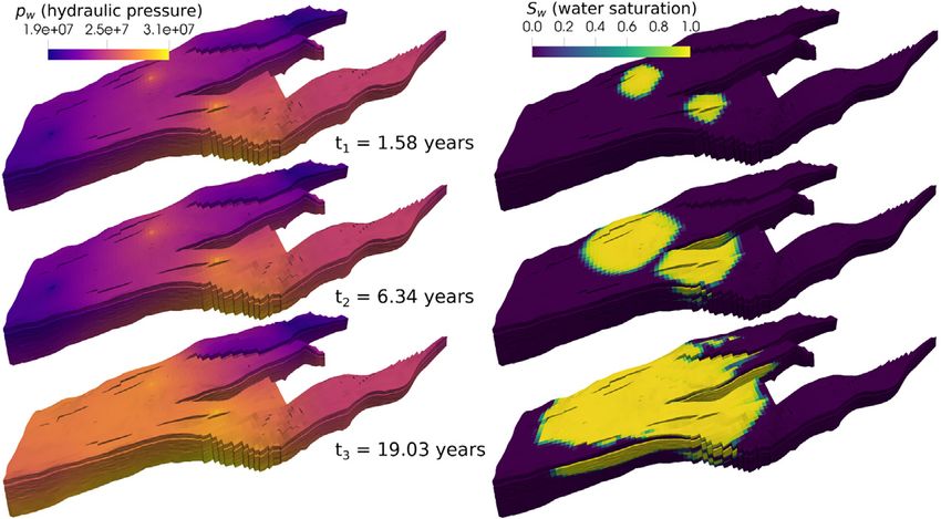
424               T. Koch, D. Gläser, K. Weishaupt et al. / Computers and Mathematics with Applications 81 (2021) 423–443

root–soil interaction [18,19], modeling of fuel cells [20], pore-network modeling [21], transport of therapeutic agents
through biological tissue [18,22–24], and subsurface–atmosphere coupling [25,26]. For a more comprehensive list of
publications that have been achieved with the help of DuMux , see dumux.org/publications.
   DuMux is based on the Distributed Unified Numerics Environment (Dune) [27–30], an open-source scientific numerical
software framework for solving partial differential equations, and is thus part of a larger community that goes beyond
the simulation of fluid–mechanical processes in porous media. Dune and DuMux are written in C++, using modern C++
programming techniques and C++ template meta programming for efficiency and generic interfaces. The Dune core
modules provide, among other things, multiple grid managers implementing a versatile common grid interface, linear
algebra abstraction and an iterative solver back-end [31], as well as abstractions facilitating parallel computing. DuMux is
designed and developed as a Dune module depending on the Dune core modules and optionally interacts with a number
of other Dune-based extension modules. The key features of DuMux are its comprehensive library of multi-phase and
multi-component flow and transport models, the flexible and modular fluid and material framework for constitutive
relations [1], abstractions for finite volume discretization schemes (see Section 3), and its focus on model coupling
(see Section 4).
   There are many other open-source projects focusing on Darcy-scale porous-medium flow and transport processes.
A list has been compiled in [32], and most references are given here again for the sake of completeness: MODFLOW,
water.usgs.gov/ogw/modflow/ [33], MRST, sintef.no/projectweb/mrst/ [34], OpenGeoSys, opengeosys.org [35], OPM, opm-
project.org [36,37], ParFlow, parflow.org [38], PFloTran, pflotran.org [39], PorePy, github.com/pmgbergen/porepy [40].
Furthermore, there are open-source numerical software frameworks with a broader focus such as deal.II, dealii.org [41],
Dune, dune-project.org [27,28], Feel++, feelpp.org [42], FEniCS, fenicsproject.org [43], MOOSE, mooseframework.org [44],
or OpenCMISS, opencmiss.org [45].
   This paper can be seen as a continuation of [1] which describes the code and the project at the beginning of the 2.X
release series. In the remainder of this introductory section, we provide a brief chronology of the development of DuMux
and some information on activities and measures that go beyond the development of the mainline code base. Section 2
introduces the general structure of the code and its design principles. Section 3 goes into more details by explaining
abstractions and software concepts for general finite volume schemes encountered in DuMux . Section 4 is devoted to
simulations coupling two or more computational domains and models. In Section 5, we briefly address new features in the
new version DuMux 3. Numerical examples that particularly highlight the strengths of the new multi-domain framework
are presented in Section 6. Finally, Section 7 discusses current limitations and perspectives.

1.1. History

    The following section briefly outlines the DuMux project history and its development. More details can be found in [32].
    The development of DuMux started at the Department of Hydromechanics and Modelling of Hydrosystems at the
University of Stuttgart (LH2) in January 2007. The software’s main goal is to facilitate research at the LH2, and provide
a framework to maintain and continuously develop research methods and results. After an initial development phase,
DuMux 1.0 was released under the GNU General Public License Version 2 (or later) [46] in July 2009.
    Since DuMux 1.0 exhibited several shortcomings regarding generality, modularity and usability, the code base was
refactored, leading to the release of DuMux 2.0 in February 2011 and an accompanying publication [1]. Since the beginning
of the 2.X release series, more emphasis was put on the sustainability of the code base and a streamlined release process.
In particular, two consecutive minor releases are to be backwards compatible in the sense that any code depending on
the previous minor release ought to work unchanged. However, compilation might emit deprecation warnings resulting
from interface changes. Since October 2013, DuMux 2.X has been semiannually released (minor releases) until release
2.12 in December 2017. Since release 2.7, Zenodo (zenodo.org) is employed to enable the citation of a specific release by
providing a digital object identifier (DOI) for each release tarball; see for example [47].
    In the 2.X release series, many improvements and enhancements, ranging from new modeling capabilities to additional
discretization schemes were introduced. Not all new features were (or could be) implemented in consistence with the
original design, leading to code which was inefficient and increasingly difficult to maintain. In November 2016, a small
team started to refactor and enhance the code base in a separate development line. Some of these changes are described
in detail in Section 2. Due to the vast amount of fundamental changes, maintaining backwards compatibility became
infeasible. Therefore, a new major release cycle was initiated.
    A preliminary DuMux version 3.0-alpha was released in December 2017 for users and developers to test and explore
the new structure and design. The new structure and several design considerations are described in Sections 2–5. Further
development, under consideration of the feedback from the DuMux community, lead to the release of DuMux 3.0 in
December 2018. In October 2019, DuMux 3.1 was released, resuming a new cycle of semiannual minor releases.

1.2. DuMux as a framework

   The main DuMux Git repository is developed and hosted at (git.iws.uni-stuttgart.de) and publicly accessible through
a GitLab server frontend. In the following, we address aspects of the DuMux research software that go beyond the
development of the main code base. After discussing quality assurance and reproducibility, we introduce the two modules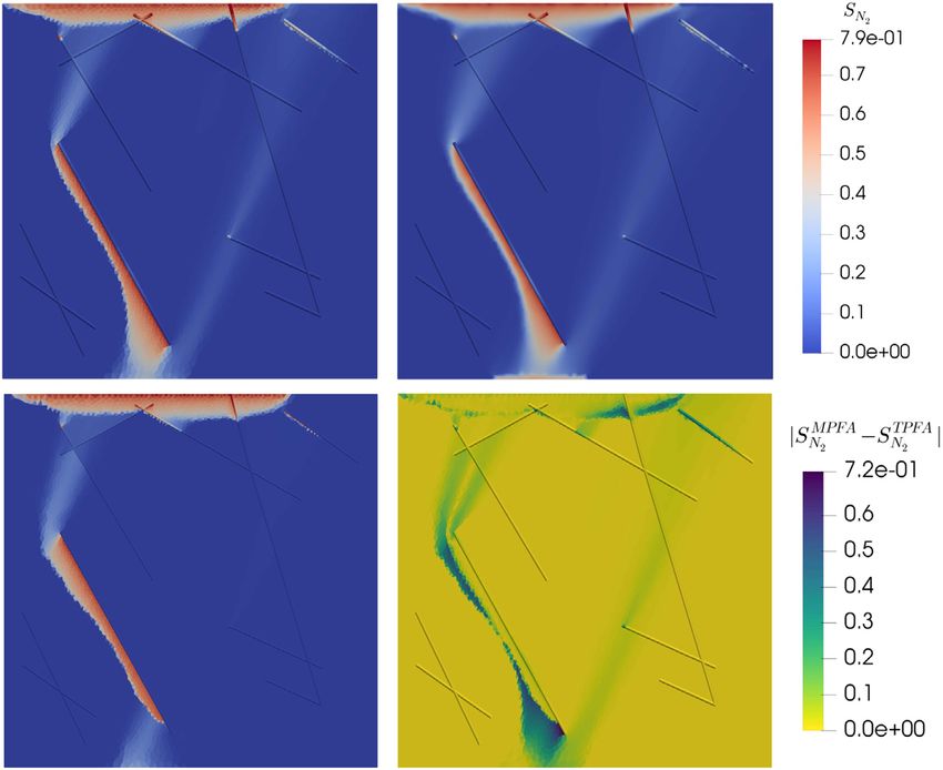
T. Koch, D. Gläser, K. Weishaupt et al. / Computers and Mathematics with Applications 81 (2021) 423–443                   425

dumux-course and dumux-lecture. More details about the development of DuMux and community building are given
in [32].
    DuMux is related to the Open Porous Media (OPM) initiative [37] which strives to develop software for ‘‘modeling
industrially and scientifically relevant flow and transport processes in porous media’’ [48]. In particular, the black-oil
simulator Flow is a main product of OPM and is built on top of the OPM modules opm-material and opm-models
(formerly ewoms). Both modules result from a fork of DuMux 2.2. DuMux can be used together with the OPM module
opm-grid which enables DuMux the use of corner-point grids—the de facto standard in the petroleum industry.
Quality assurance and reproducibility. Automated testing is indispensable for the sustained development of software [49].
Currently, there exist more than 400 unit and system tests for DuMux . The test suite is built and executed by a BuildBot
CI server at git.iws.uni-stuttgart.de/buildbot in an automated way, triggered by each commit to the master branch of
the DuMux Git repository. We regularly assess that the tests cover a large number of lines of code and work towards
increasing the coverage.1 To ensure the quality of newly developed capabilities and features, every corresponding addition
to the code base is to be accompanied by a test and documented appropriately. Moreover, each code change is reviewed
by at least one other developer in a transparent and public review process using GitLab.
   In addition to assuring quality of the code base, research results published with the help of DuMux should be
reproducible. To this end, the project DuMux -Pub was initiated in 2015. It provides the capabilities to archive and
document code used in scientific publications. A few simple tools automate the process from a DuMux application to a new
light-weight Dune module containing the source and data files required to reproduce the research results. Furthermore,
the required versions of all dependencies are automatically determined and documented. At the LH2 department, all
relevant scientific articles, as well as bachelor’s, master’s and doctoral theses, are accompanied by a DuMux -Pub module
hosted at git.iws.uni-stuttgart.de/dumux-pub [32]. As part of the ongoing project ‘‘Sustainable infrastructure for the
improved usability and archivability of research software on the example of the porous-media-simulator DuMux ’’ (SusI),2
these existing measures will be extended by automating the generation of Docker containers for DuMux -Pub modules
and the creation of web applications in order to easily reproduce the research results.
DuMuX course. The dumux-course module has been created for a DuMux course offered 2018 in Stuttgart. It is
continuously improved and enhanced along with the mainline development. While the module is used in conventional
DuMux courses with participants attending personally [32], it is also designed to be used independently by everyone who
would like to learn how to work with DuMux . All course exercises are documented and contain task descriptions and
solutions. Their contents range from a very basic first building and running experience to fairly advanced applications
based on coupled model equations. The module also contains the slides from the course providing broader context and
background information.
DuMuX lecture. The LH2 department offers Master level courses for different study programs (Environmental and Civil
Engineering, Water Resources Engineering and Management, Simulation Technology, or Computational Mechanics of
Materials and Structures), where computer exercises using DuMux are an essential component. The module dumux-
lecture contains all example applications used in these lectures, with most of the applications belonging to the lecture
‘‘Multiphase Modeling’’. Each application has its own folder containing problem setup and spatial parameter specifications,
as well as an input file where typically those runtime parameters can be specified that are of educational value for the
problem. Each example is accompanied by explanations and tasks.

2. Structure and design principles

   DuMux is designed as a research code framework. Foremost, this means that it is designed with an emphasis on
modularity. DuMux user code is usually developed in a separate Dune module that lists DuMux as its dependency. To
maintain flexibility for a user, DuMux follows the principle that all components of a simulation should be easily replaceable
with a new implementation, without modifying code in the DuMux module itself. For example, it is simple to change from
one of the implemented capillary–pressure relationships to a custom function, to modify the numerical flux computation,
and to change from a cell-centered to a vertex-centered finite volume discretization. DuMux profits from the modular
design of Dune. For example, an unstructured grid implementation can be exchanged for an efficient structured grid
implementation by changing a single line in the user code.
   To maintain computational efficiency, much of the modularity is realized through the use of C++ templates and generic
programming techniques such as traits and policies. Moreover, the developers of DuMux try to follow well-known object-
oriented design principles and the separation of algorithms and data structures, as for example in the design of the DuMux
material framework [50]. DuMux 3, which requires a C++14-compatible compiler, increasingly makes use of modern C++
features such as lambdas, type deduction, or smart pointers, to the benefit of usability, modularity, and efficiency.
   In the DuMux environment, the term model is used to describe a system of coupled partial differential equations (PDEs)
including constitutive equations needed for closure. Many models, in particular PDEs describing general non-isothermal

  1 A detailed weekly coverage report created with gcov, gcovr and GitLab CI is publicly available at pages.iws.uni-stuttgart.de/dumux-repositories/
dumux-coverage/.
  2 Funded by the German Research Foundation (DFG).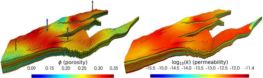
426                 T. Koch, D. Gläser, K. Weishaupt et al. / Computers and Mathematics with Applications 81 (2021) 423–443

multi-component multi-phase flow processes in porous media, are already implemented in DuMux . Furthermore, a user
can choose from a variety of constitutive laws to describe closure relations, and multiple fluid and solid systems and
components. More importantly, the code design also facilitates using custom implementations.
   The main components of a DuMux simulation are represented in the code by corresponding C++ classes. When using
one of the implemented models out-of-the-box, a user usually implements at least two such classes in addition to the
program’s main function. The Problem class defines boundary conditions, initial conditions (if necessary), and volumetric
source terms (if any), by implementing a defined class interface. The SpatialParams class defines the spatial distribution
of material parameters, such as porosity, permeability, or for example, parameters for the van Genuchten water retention
model (if applicable). The Problem class stores a pointer to an instance of the SpatialParams class. Moreover, each
simulation currently creates at least one tag (a C++ struct) which is used to specify several compile time options (properties)
of the simulation by means of partial template specialization. Code Example 1 shows how to set properties for a newly
defined tag. Properties can be extracted as traits of such a tag in other parts of the code. Depending on the chosen model,
more of such properties have to be defined and examples are provided for all existing models in DuMux . User defined
models can provide their own properties.
 1    namespace Dumux {
 2    namespace Properties {
 3
 4    // create a new type tag
 5    namespace TTag {
 6    struct Example { using InheritsFrom = std :: tuple ; };
 7    } // end namespace TTag
 8
 9    // set the Dune grid type
10    template  struct Grid
11    { using type = Dune :: UGGrid ; };
12
13    // set the problem type
14    template  struct Problem
15    { using type = UserProblem ; };
16
17    // set the spatial parameters type
18    template
19    struct SpatialParams
20    { using type = UserSpatialParams ; };
21
22    // set the fluid system type
23    template  struct FluidSystem
24    { using type = FluidSystems :: OnePLiquid ; };
25
26    } // end namespace Properties
27    } // end namespace Dumux

Code Example 1: An example of a property setting for DuMux 3. The simulation is configured to use a one-phase porous
medium model (OneP), a cell-centered two-point-flux-approximation discretization scheme (CCTpfaModel), and liquid
water as a fluid. The UserProblem and UserSpatialParams types are implementation- and user-defined. Header
includes are omitted for brevity. The types attached to the Example tag, can be extracted as traits, see GetPropType
in Code Example 2.

    A rather significant improvement in DuMux 3 concerns the way the program’s main function is written. In DuMux 2,
the main function called a predefined start function that determined the program flow. Modifications to the program
flow were made possible by numerous hook functions. For example, the Problem base class implemented a hook function
postTimeStep that could be overloaded by the user’s Problem implementation, injecting the notion of time and program
flow into the Problem class; a hook function addVtkOutputFields injected a notion of file I/O. This design concept
introduced many dependencies between classes and (as shown here for the Problem class) lead to the violation of the
well-known single responsibility principle, hindering modular design. Furthermore, due to the concept of hook functions,
it was very difficult to write simulations outside the predefined program flow in start. For example, all simulations were
considered transient and non-linear. Consequently, solving stationary equations was often realized by solving a single time
step and making sure that the assembled storage term is zero. Solving linear equations was realized by executing a single
iteration of a Newton method. On the positive side, a user had the possibility to realize most changes within a single
header file.
    In contrast, the program’s main function in DuMux 3 contains all of the main steps of the simulation, see Code
Example 2. Therefore, to solve a stationary PDE, the TimeLoop instance (l. 41) and the time loop (l. 53ff) can simply be
removed from the program flow. Similarly, the NewtonSolver class can be replaced by a LinearPDESolver to solve a
linear PDE. Finally, the I/O logic and other modifications to the main program flow can be directly written inside the main
function. As a result, the main program flow becomes arguably more transparent, which has been confirmed by feedback
from the DuMux user community. For more information on the steps of a DuMux simulation, we refer the interested
reader to the DuMux handbook [51].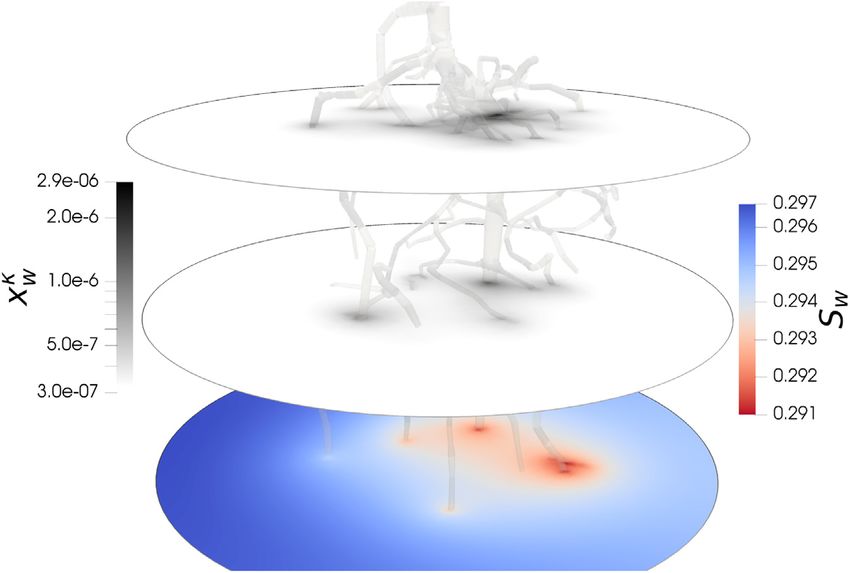
T. Koch, D. Gläser, K. Weishaupt et al. / Computers and Mathematics with Applications 81 (2021) 423–443   427

 1   int main(int argc , char ** argv)
 2   {
 3     using namespace Dumux ;
 4
 5       // an example tag from which multiple traits
 6       // can be extracted (see GetPropType below )
 7       using Tag = Properties :: TTag :: Example ;
 8
 9       // initialize MPI ( enables parallel runs)
10       Dune :: MPIHelper :: instance (argc , argv);
11
12       // parse command line arguments and a parameter file
13       Parameters :: init(argc , argv , "params . input ");
14
15       // create a Dune grid (from information in the parameter file)
16       using Grid = GetPropType ;
17       GridManager  gridManager ; gridManager .init ();
18
19       // create the finite volume grid geometry (see Section 3)
20       const auto leafGridView = gridManager .grid (). leafGridView ();
21       using GridGeometry = GetPropType ;
22       auto fvGridGeometry = std :: make_shared < GridGeometry >( leafGridView );
23       fvGridGeometry -> update ();
24
25       // the problem ( initial conditions , boundary conditions , sources )
26       using Problem = GetPropType ;
27       auto problem = std :: make_shared ( fvGridGeometry );
28
29       // the solution vector , set to the initial solution
30       using SolutionVector = GetPropType ;
31       SolutionVector x; problem -> applyInitialSolution (x);
32       auto xOld = x;
33
34       // the grid variables ( secondary variables on control volumes and faces )
35       using GridVariables = GetPropType ;
36       auto gridVariables = std :: make_shared < GridVariables >( problem , fvGridGeometry );
37       gridVariables ->init(x);
38
39       // get some time loop parameters and instantiate time loop
40       const auto tEnd = getParam ( "TimeLoop .TEnd ");
41       auto dt = getParam ( "TimeLoop . DtInitial ");
42       auto timeLoop = std :: make_shared (0, dt , tEnd);
43
44       // the assembler with time loop for transient problem & the solver
45       using Assembler = FVAssembler ;
46       auto assembler = std :: make_shared ( problem , fvGridGeometry , gridVariables , timeLoop );
47       assembler -> setPreviousSolution (xOld);
48       Dumux :: NewtonSolver  nonLinearSolver (assembler , linearSolver );
49
50       // initialize output module
51       ...
52
53       // time loop
54       timeLoop -> start (); do
55       {
56         // solve the non - linear system with time step control
57         nonLinearSolver . solve (x, * timeLoop );
58
59         // make the new solution the old solution
60         xOld = x; gridVariables -> advanceTimeStep ();
61
62         // advance the time loop to the next step
63         timeLoop -> advanceTimeStep ();
64
65         // report statistics of this time step
66         timeLoop -> reportTimeStep ();
67
68         // write output , set new time step size
69         ...
70
71       } while (! timeLoop -> finished ());
72
73       return 0;
74   }

Code Example 2: An example of a main function using DuMux 3 for solving a transient non-linear problem with a finite
volume scheme and numeric differentiation. The simulation can be run in parallel (MPI, distributed memory). Header
includes are omitted for brevity.
428                    T. Koch, D. Gläser, K. Weishaupt et al. / Computers and Mathematics with Applications 81 (2021) 423–443

3. Abstractions and concepts for general finite volume schemes

    One of the most important abstractions in DuMux is the grid geometry. The concept partly existed in DuMux 2 but
was significantly redesigned and has been casted into an object-oriented representation in DuMux 3. A grid geometry is
a wrapper around a grid view on a Dune grid instance. Dune grids are general hierarchical grids and grid views provide
read-only access to certain parts of the grid. In particular, a leaf grid view is a view on all grid entities without descendants
in the hierarchy (which are not refined), thus covering the whole domain (in sequential simulations) or the part of the
grid assigned to a single processor (in parallel simulations), while a level grid view is a view on all entities of a given level
of the refinement hierarchy. The grid geometry constructs, from such a grid view, all the geometrical and topological data
necessary to evaluate the discrete equations resulting from a given finite volume scheme. This abstraction allows us to
implement many different finite volume schemes in a unified way. In the following sections, we will present and motivate
the mathematical abstractions behind the grid geometry concept, describe their realizations in the code in form of C++
classes and provide an exemplary code snippet that illustrates how to use them.

3.1. Finite volume discretization

   Let us consider a domain Ω ⊂ Rn , 1 ≤ n ≤ 3, with boundary ∂ Ω , which is further decomposed into two subsets on
which Dirichlet and Neumann boundaries are specified, that is ∂ Ω = ∂ ΩD ∪ ∂ ΩN . Furthermore, let us consider a general
conservation equation,
      ∂m
         + ∇ ·ψ = q,                                                                in Ω ,                                       (3.1a)
      ∂t
                  ψ · n = gN ,                                                      on ∂ ΩN ,                                    (3.1b)

                     u = uD ,                                                       on ∂ ΩD ,                                    (3.1c)

              u(t = 0) = u0                                                         in Ω ,                                       (3.1d)

where m = m(u) is the conserved quantity depending on the primary variable u, ψ = ψ (u) is a flux term and q = q(u) a
source term. All terms may non-linearly depend on u. Eqs. (3.1a)–(3.1d) constitute a non-linear problem in u with initial
and boundary conditions.
                                                                                    ⋃
    We introduce the primary grid M with elements E ∈ M, such that Ωh =                E ∈M E is a discrete approximation of
                                                                          ⋃
Ω . Furthermore, we introduce a tessellation T of Ω , such that Ωh = K ∈T K , where each K ∈ T is a control volume
with measure |K | > 0. The control volumes K do not necessarily need to coincide with the elements E. However, for
cell-centered finite volume schemes, usually T ≡ M. Each control volume is partitioned into sub-control-volumes κ ,
where κ = K is one admissible partition. Moreover, the boundary of the control volume ∂ K consists of a finite number
of faces f ⊂ ∂ K which are either inner faces fI = ∂ K ∩ ∂ L, where L ∈ T is an adjacent control volume, or boundary faces
fB = ∂ K ∩∂ Ωh . Depending on the discretization method, it may be useful to partition the faces f into sub-(control-volume)-
                                                                                                                     ⋃
faces σ . We denote by EK the entire set of such sub-faces on ∂ K , forming a disjoint partition such that ∂ K = σ ∈E σ .
                                                                                                         ⋃                K
Accordingly, TK denotes the set of sub-control volumes embedded in a control volume K with K = κ∈T κ .
                                                                                                               K
    Integration of Eq. (3.1a) over a control volume and application of the divergence theorem yields
      ∫               ∑∫             ∫
              ∂m
                 dx +      ψ · n dΓ = q dx,                                                                                       (3.2)
          K   ∂t         f             K
                       f ⊂∂ K

where n is a unit outer normal vector on ∂ K . Using the concept of sub-control-volumes and sub-control-volume-faces,
allows to reformulate Eq. (3.2) as
      ∑ ∫ ∂m        ∑∫                ∑∫
               dx +        ψ · n dΓ =       q dx.                                                                                 (3.3)
      κ∈T κ ∂t      σ ∈E σ            κ∈T κ
              K                  K                      K
                                                                                                          ∫
   Let us now replace the exact flux over sub-face σ by the approximation FK ,σ ≈ σ ψ · n dΓ and approximate the
volume integrals in Eq. (3.3) to arrive at the discrete, control-volume-local formulation of Eq. (3.1a),
      ∑ mt +∆t − mt   ∑            ∑
          κ       κ
                    +      FK ,σ −     qκ = 0,                                                                                    (3.4)
      κ∈T
             ∆t       σ ∈E         κ∈T
              K                      K            K
T. Koch, D. Gläser, K. Weishaupt et al. / Computers and Mathematics with Applications 81 (2021) 423–443                     429

Fig. 1. Illustration of the configurations of control volumes and sub-faces on a computational grid for different discretization schemes. The tpfa and
mpfa scheme use the grid elements as control volumes (E ≡ K ≡ κ ), while in the box scheme the control volume is constructed around the grid
vertices by connecting the barycenters of all adjacent geometrical entities. The partition of the boundary ∂ K by the sub-faces σ is illustrated by
depicting the corners of each sub-face.

where the approximate integrals mκ and qκ depend on the specific finite volume method. The time derivative is
approximated by a backward or forward finite difference,3 determining the time level t or t + ∆t at which the flux
and source terms FK ,σ and q are evaluated. The expressions for the discrete fluxes FK ,σ depend on the actual underlying
finite volume scheme. Fore more detailed information, we refer to [52,53] for the box scheme, and [54] for two-point and
multi-point-flux-approximation finite volume schemes (tpfa and mpfa).
    If a backward Euler time discretization is chosen, the nonlinear system corresponding to Eq. (3.4) on each control
volume K is solved by Newton’s method. In each Newton step n, we compute a linearized discrete PDE system in residual
form
       A(un )∆u = A(un )(un − un+1 ) = r(un ),                                                                                                  (3.5)
                                                                                                          ∂r
where u now is the vector of primary variables for each degree of freedom, and A =            is the Jacobian of the residual r,
                                                                                                          ∂u
i.e. the discrete equation evaluated at un . The residual for a control volume K ∈ T is given by the left-hand-side of Eq. (3.4).
In the default configuration, the derivatives in the Jacobian matrix are approximated by numerical differentiation in
DuMux .

3.2. Element-wise assembly

    Dune grids and the connectivity information provided by the grid are rather element-centered (elements are grid
entities of co-dimension 0). For this reason, it is natural in Dune to choose an element-wise assembly of the residual. The
choice of T and hence the sub-control-volumes κ and sub-control-volume-faces σ is motivated by the goal of a convenient
implementation of an element-wise assembly for a given control volume scheme. Fig. 1 depicts the configurations of
control volumes and sub-faces as chosen in DuMux , exemplarily for the tpfa, mpfa and the box scheme. A corresponding
illustration for the mac scheme can be found, for example, in [55]. As illustrated in Fig. 1, the sub-control-volumes for
the box scheme are chosen such that the residual associated with a degree of freedom on a vertex can be split into
contributions from all neighboring elements. For the mpfa-o scheme, the sub-faces are defined such that each sub-face can
be associated to a grid vertex. This is motivated by the fact that the expressions for the discrete fluxes across the sub-faces
depend on the degrees of freedom within so-called interaction regions, constructed around the grid vertices [56].

3.3. Representation in the software implementation

   Sub-control-volumes κ and sub-control-volume-faces σ , as introduced in Section 3.1, are represented in the code by
objects of the classes SubControlVolume and SubControlVolumeFace. Depending on the caching model, which can be
selected by specifying a template argument, these objects are either stored in the GridGeometry instance, or constructed
on-the-fly on a per-element basis during the assembly. Furthermore, DuMux has the notion of a local view on the grid
geometry. The local view is an element-centered view that gives access to all κ and σ on an element, as well as all
connectivity and geometry information to assemble storage, flux, and source terms. For example, for a tpfa scheme, the
neighboring control volumes and associated primary and secondary variables have to be accessed to calculate the fluxes
over the control-volume interfaces. Code Example 3 shows how to assemble the total mass contained in a domain for
a given grid M. The presented code is identical for all introduced finite volume schemes. Similar to the range-based-
for syntax to iterate over all elements of a grid view provided by Dune, the local view on the grid geometry in DuMux
makes it possible to iterate over all sub-control-volumes associated with an element in a concise and readable way (l. 17).
Analogously, a range-generator for iterating over all sub-control-volume-faces associated with an element is provided.

  3 DuMux currently only implements the backward and forward Euler time discretization schemes.
430                   T. Koch, D. Gläser, K. Weishaupt et al. / Computers and Mathematics with Applications 81 (2021) 423–443

Fig. 2. Different types of model coupling in DuMux multi-domain simulations. (a) multi-physics models (on the same grid), (b) multiple
non-overlapping domains with sharp conforming or non-conforming interface, (c) multiple overlapping domains with different discretizations,
(d) conforming and non-conforming (embedded) mixed-dimensional domains (1D–2D, 1D–3D, 2D–3D). The different coupling modes can also be
combined. Typical mixed-dimensional simulations also solve multi-physics problems, or use different discretization schemes in the subdomains. The
number of subdomains is not limited to two.

 1    const double porosity = 0.4;
 2    const double density = 1000.0;
 3    double totalWaterMass = 0.0;
 4
 5    // iterate over all elements of the leaf grid view of the grid
 6    for (const auto& element : elements ( leafGridView ))
 7    {
 8        // construct a local view on the grid geometry
 9        auto fvGeometry = localView (* fvGridGeometry );
10
11        // the view has to be bound to the current element
12        // this is a no -op if the geometry is cached
13        fvGeometry .bind( element );
14
15        // iterate over all sub -control - volumes in the local view
16        // and accumulate the mass
17        for (const auto& scv : scvs( fvGeometry ))
18            totalWaterMass += saturation [scv. dofIndex ()] * porosity
19                              * density * scv. volume ();
20    }
21
22    std :: cout
T. Koch, D. Gläser, K. Weishaupt et al. / Computers and Mathematics with Applications 81 (2021) 423–443 431
3 // with respect to degrees of freedom in domain j
4 template
5 const std :: vector &
6 couplingStencil (Dune :: index_constant domainI ,
7 const Element & elementI ,
8 Dune :: index_constant domainJ ) const;
Code Example 4: The member function couplingStencil has to be implemented by all deriving coupling manager
implementations. The template arguments i and j are the indices of one pair of coupled subdomains. They are deduced
from the two index objects domainI and domainJ, passed as arguments to the function. In case two subdomain are not
coupled, the function is required to return a reference to an empty stencil vector. For domain i, an instance of the element
is passed, for which the residual in the element-wise assembly is to be computed. The function returns a vector of all
indices of degrees of freedom coupled to one of the degrees of freedom associated with element elementI.
Moreover, the coupling manager has to transfer data between the sub-problems. This general concept can be used to
implement a wide class of coupling schemes. Finding the coupling stencils often involves intersecting two grids. For this
purpose, DuMux provides efficient intersection algorithms based on axis-aligned bounding box volume hierarchy data
structures [60,61] computed for Dune grids. Code Example 5 shows how to intersect two given grid geometries and use
the connectivity information to construct a coupling stencil, that can be used, for example, in a non-conforming embedded
fracture model.4 The grid intersection and stencil computation is illustrated in Fig. 3.
1
2 // which degrees of freedom of the other domain does the element residual depend on?
3 using Stencils = std::vector;
4 Stencils lowDimCouplingStencils , bulkCouplingStencils ;
5 // resize to the number of grid elements
6 lowDimCouplingStencils . resize ( lowDimGridGeometry . gridView ().size(/* codim =*/ 0));
7 bulkCouplingStencils . resize ( bulkGridGeometry . gridView ().size(/* codim =*/ 0));
8
9 // intersect two grid geometries
10 // we choose domain ( first argument ): lowDim , target ( second argument ): bulk
11 // see
12 const auto glue = makeGlue ( lowDimGridGeometry , bulkGridGeometry );
13
14 // interate over all intersections
15 for (const auto& is : intersections (glue))
16 {
17 // the element index of the lowDim element of this intersection
18 const auto domainIdx = lowDimGridGeometry . elementMapper (). index (is. domainEntity ());
19 // there might be multiple bulk elements associated with this intersection
20 for ( unsigned int i = 0; i < is. numTargetNeighbors (); ++i)
21 {
22 // the element index of the bulk element of this intersection
23 const auto targetIdx = bulkGridGeometry . elementMapper (). index (is. targetEntity (i));
24 // insert target - domain index pair into the respective stencil
25 lowDimCouplingStencils [ domainIdx ]. insert ( targetIdx );
26 bulkCouplingStencils [ targetIdx ]. insert ( domainIdx );
27 }
28 }
Code Example 5: Sample code which intersects two grid geometries (see Section 3.1) and uses the resulting connectivity
information to construct coupling stencils for a cell-centered finite volume scheme. A bulk grid (bulk) is intersected
with an overlapping grid with lower dimension (lowDim) which may discretize a three-dimensional rock domain and a
network of two-dimensional fractures. (The code snippet is identical for 3D–2D and 2D–1D.) An intersection is Γ = Eb ∩ El ,
where Eb (targetEntity) is an element of the bulk grid and El (domainEntity) an element of the lower-dimensional
embedded grid. If there exist multiple such intersections with identical geometry (e.g. a fracture element coincides with
a face shared by two bulk elements), they are represented in the code by a single intersection object with access to all
elements (‘‘entities’’) associated with the intersection (‘‘neighbors’’). The interface of the glue object is similar to that
implemented in the Dune module dune-grid-glue [62] which implements an advancing front algorithm instead of an
algorithm based on spatial data structures used here.
4 The DuMux code for such a simulation (2D–3D embedded fracture model) can be found in the DuMux repository under test/multidomain/
embedded/2d3d/1p_1p.432 T. Koch, D. Gläser, K. Weishaupt et al. / Computers and Mathematics with Applications 81 (2021) 423–443
Fig. 3. Determination of the coupling stencil for an embedded fracture model using a cell-centered finite volume scheme. One grid, M1 = T1 =
{K , L, M }, consists of three squares (black), and a second grid, M2 = T2 = {A, B, C , D, F }, consists of five segments (blue). Intersections between the
grid element are highlighted in green. Each element E ∈ Mj , j ∈ {1, 2}, is associated with a degree of freedom uE with index iE , and an element
residual rE , see Eq. (3.5). The element residual is a function of degrees of freedom of both domains. The indices of these degrees of freedom are
collected in the stencil SE (same domain) and the coupling stencil SEc (other domain). For the presented example, SL = {iK , iL , iM }, SLc = {iC , iD }
(bulk coupling stencil in Code Example 5), SD = {iC , iD , iF }, SDc = {iL , iM } (lowdim coupling stencil in Code Example 5), and analogously for all other
elements. (For interpretation of the references to color in this figure legend, the reader is referred to the web version of this article.)
Furthermore, DuMux provides an assembler class for multi-domain models, which assembles the discrete PDE system
in residual form
A1 C12 ... C1n ∆ u1 r1
⎡ ⎤⎡ ⎤ ⎡ ⎤
⎢C21 A2 ⎥ ⎢ ∆ u2 ⎥ ⎢r 2 ⎥
⎢ .
⎣ . .. ⎥⎢ . ⎥ = ⎢ . ⎥,
⎦⎣ . ⎦ ⎣ . ⎦ (4.1)
. . . .
Cn1 An ∆ un rn
where Ai is the Jacobian of the discrete PDE system for subdomain i, and Cij is the coupling Jacobian with derivatives
∂r
of residuals of domain i with respect to degrees of freedom of domain j, Cij = ∂ ui . The assembler class and the matrix
j
class are generic, so that the sub-vectors ui and sub-matrices Ai can themselves have a block structure, and support an
arbitrary number of subdomains. The block structure can be exploited, for example, for constructing preconditioners for
a monolithic solver, or to algebraically implement schemes where the subdomain systems are solved successively in an
iterative algorithm.
The presented multi-domain concept has been successfully used to implement models with coupled flow and transport
processes in vascularized brain tissue [23,63], root–soil interaction models in the vadose zone [18], flow and transport
models for fractured rock systems [12,64], coupled porous medium flow and atmosphere flow (Darcy–Navier–Stokes) at
the soil surface [55], and a model that couples a pore-network model with a Navier–Stokes model [21].
5. New features in DuMux 3
Numerous new features are added in DuMux 3 in comparison with the 2.X series. We briefly mention the most
important changes. A complete redesign of many high-level class abstractions such as assembler, linear and non-linear
solvers, grid readers and grid geometry, and file I/O leads to more readable and flexible main functions, see also Section 2.
The numerous models are improved in terms of code reuse and modularity, so that code duplication is minimized and
readability improved. In addition to the fluid system concept, a solid system concept is introduced, which facilitated the
implementation of new models including mineralization or precipitation of substances that potentially modify the porous
matrix structure [17,65]. Porous material properties such as intrinsic permeability and porosity can be implemented
to depend (linearly or non-linearly) on the primary variables. We generalized thermal and chemical non-equilibrium
models to be combinable with any porous medium model. Multi-component diffusion can now be modeled by Maxwell–
Stefan diffusion. A versatile implementation of cell-centered mpfa-o scheme is now usable with all models [12]. The
Navier–Stokes models are redesigned to use a mac scheme on a staggered grid [21,55,66], including a Reynolds-averaged
Navier–Stokes model [67,68] with a variety of turbulence models (e.g. k − ϵ , k − ω), as well as a second-order upwind
scheme. We can now solve problems based on the two-dimensional shallow water equations. Finally, the multi-domain
module adds the functionality of versatile model coupling as described in Section 4.
6. Numerical examples
Previous versions of DuMux have been developed with a strong focus on multi-phase flow and transport in porous
media [1]. The quality of the multi-phase flow models has been maintained or improved5 in version 3. As an example,
we present a two-phase flow scenario based on the Norne data set.6 The porosity field, the isotropic heterogeneous
5 We refer to the DuMux changelog (https://git.iws.uni-stuttgart.de/dumux-repositories/dumux/blob/master/CHANGELOG.md).
6 Norne data set obtained from the module opm-data (Open Database License, https://github.com/OPM/opm-data).T. Koch, D. Gläser, K. Weishaupt et al. / Computers and Mathematics with Applications 81 (2021) 423–443 433 Fig. 4. Porosity and permeability field of the Norne formation. Permeability is isotropic and values are given in m2 . The left image additionally highlights the elements of the grid and displays the location of the injection (blue) and production wells (brown). (For interpretation of the references to color in this figure legend, the reader is referred to the web version of this article.) Fig. 5. Evolution of the wetting phase pressure (in Pa) and saturation. This is a new visualization of the data obtained with DuMux by Schneider et al. [58], based on the injection scenario originally presented in [70]. permeability field, the elements E of the computational grid M, and the injection and extraction wells are shown in Fig. 4. The computational domain is represented by a corner-point grid [69,70], using the dedicated Dune grid interface implementation of opm-grid [37]. The incompressible immiscible two-phase model equations and parameters are given in [70, Eqs. (56)–(60) and Table 3]. The nonlinear coupled PDEs are discretized with a tpfa cell-centered finite volume scheme in space and a backward Euler scheme in time. Initially, the domain is fully saturated with oil. Water is injected through two wells. Two extraction wells initially produce oil and an oil–water mixture at later times. The wells are modeled by fixed bore-hole pressures using a Peaceman well model [71]. The temporal evolution of the wetting phase pressure and saturation is shown in Fig. 5. The development of DuMux 3 has been particularly driven by a focus on model coupling. In the remainder of this section, three numerical examples demonstrate the flexibility of the new multi-domain framework in DuMux 3. In Section 6.1, free flow over a porous medium is modeled by coupling a Navier–Stokes model to a pore-network model. The domains are coupled at a common interface. Section 6.2 shows a simulation of two-phase flow in a fractured rock matrix. The fracture flow is computed on lower-dimensional domains conforming with the control-volume faces of the three-dimensional rock matrix domain discretization, which allows to model highly conductive fractures as well as impermeable fractures. The example shows the differences between a tpfa and an mpfa-o finite volume scheme for a rock matrix with anisotropic permeability. Finally, an example of root water uptake and tracer transport is given in Section 6.3. The roots are represented by a network of tubes embedded into the soil matrix. The mass exchange between the two non-conforming domains is realized with adequate source terms. The source code for these examples as well as instructions for the reproduction of the results can be found in the DuMux -pub module to this publication at git.iws.uni-stuttgart.de/dumux-pub/dumux2019. For pre- and post-processing of DuMux simulation results, we advertise a workflow based on a number of external open source tools such as Gmsh [72] (meshing), Gnuplot [73] and Matplotlib [74] (plotting), and ParaView [75] (visualization). The latter has been used to create the visualizations in Figs. 4–7, 9 and 10.
434                    T. Koch, D. Gläser, K. Weishaupt et al. / Computers and Mathematics with Applications 81 (2021) 423–443

Fig. 6. Velocity fields for the three scenarios. Re is based on the averaged velocity within the channel. Note the different color scale for the network
in the third scenario (bottom). pout = 0. (For interpretation of the references to color in this figure legend, the reader is referred to the web version
of this article.)
Source: Figure adapted from [21] (license: CC BY 4.0).

                           Fig. 7. Distribution of the mole fraction xt for the three different scenarios at different times.
                           Source: Figure adapted from [21] (license: CC BY 4.0).
T. Koch, D. Gläser, K. Weishaupt et al. / Computers and Mathematics with Applications 81 (2021) 423–443 435
Fig. 8. Domain and Dirichlet boundary conditions for the two-phase flow example through fractured porous media. The subscript hs refers to
hydrostatic pressure conditions.
Fig. 9. Nitrogen saturation distribution at the final simulation time t = 75 000 s obtained with the mpfa-o scheme (upper left), the box scheme
(upper right) and the tpfa scheme (lower left) for the example application of two-phase flow through a fractured porous medium. The lower right
image shows the difference in the saturations obtained with the mpfa-o and the tpfa scheme.
6.1. Coupling a free flow model with a pore-network model
This example is adapted from [21], where a coupled model of free channel flow adjacent to a porous medium is
presented with a detailed model description. We model transient multi-component flow over a random porous structure
in a two-dimensional model domain. The channel flow is governed by the Navier–Stokes equations, neglecting gravity
and dilatation [76],
∂ (ρ v)
+ ∇ · ρ vvT = ∇ · µ ∇v + (∇v)T − ∇p,
( ) [ ( )]
(6.1)
∂t436 T. Koch, D. Gläser, K. Weishaupt et al. / Computers and Mathematics with Applications 81 (2021) 423–443
Fig. 10. Simulation of root-water uptake of a white lupin and simultaneous tracer transport in the soil, shown at t = 3 d. Three horizontal cuts
through the soil domain are shown. The tracer, with mole fraction xκw , is not taken up by the roots and accumulates, particularly where the root
water uptake rate is highest. On the bottom slice, the water saturation Sw is shown. The saturation slightly decreases close to the roots. Its spatial
gradient depends on the flow resistances in soil and root, the current water distribution, and the prescribed transpiration rate rT .
with the fluid density ρ , the fluid velocity v, the fluid pressure p, and the dynamic viscosity µ. A molar balance equation
for each component κ ,
∂ (ρm xκ )
+ ∇ · (ρm xκ v − Dρm ∇xκ ) = 0, (6.2)
∂t
models advective and diffusive transport of the fluid components, where xκ is the component mole fraction, ρm the fluid
molar density, and D the binary diffusion coefficient. Diffusive fluxes are described by Fick’s law.
For modeling flow and transport in the porous medium, a pore-network model is used [77,78]. The complex pore-
scale geometry of the porous medium is transferred to a simplified geometry, the pore bodies and pore throats. For each
component κ , Eq. (6.2) is formulated discretely on each pore body where the primary variables are located. The advective
and diffusive fluxes are evaluated on the pore throats. We refer to [21] for further details.
Coupling conditions are formulated at the interface between the two models to ensure thermodynamic consistency.
At the locations where no throat intersects with the interface, a no-flow/no-slip condition for the Navier–Stokes model is
enforced. At the actual intersections, we prescribe the continuity of normal forces [79] resulting in a Neumann boundary
condition for the free flow domain,
) )]ff
ρ vvT − µ ∇v + (∇v)T + pI n = [p]pnm ,
[(( ( )
n· (6.3)
where the superscripts ff and pnm mark quantities of the free-flow and pore-network model, respectively. We use the
tangential part of the average velocity within the throat at the boundary [v]pnm as a slip condition for the free flow,
{ pnm
[v] · [t]ff on pore throat,
[v · t]ff = (6.4)
0 else,
where [t]ff is a unit tangential vector to the coupling interface.
The velocity within the throat is given by
Qt
[v]pnm = nt , (6.5)
At
where Qt is the volume flow within the throat, At is its respective cross-sectional area and nt is a unit vector parallel to
the pore throat, pointing towards the coupling interface. Finally, we require the conservation of mass
[(ρm xκ v − Dρm ∇ xκ ) · n]ff = −[(ρm xκ v − Dρm ∇ xκ ) · n]pnm (6.6)
and enforce the continuity of mole fractions at the interface,
[xκ ]ff = [xκ ]pnm . (6.7)T. Koch, D. Gläser, K. Weishaupt et al. / Computers and Mathematics with Applications 81 (2021) 423–443 437
The Navier–Stokes equations are discretized with a mac scheme on a staggered grid. The pore-network model is also
implemented in DuMux and will become part of stable code basis in an upcoming release. The pore-network is described
as a one-dimensional network embedded in a two-dimensional domain, using the Dune grid implementation dune-
foamgrid [80]. We used the DuMux multi-domain framework in order to achieve a fully monolithic coupling between
the two sub-models. Since only elements on the domain boundary are coupled in this example, we employed a simplified
intersection algorithm for creating the coupling stencils in comparison with Code Example 5. Instead of intersecting the
entire grid, only the end points (boundary pores) of the pore-network grid geometry are intersected with the channel
domain grid geometry to compute the coupling stencils. Furthermore, for the staggered grid discretization, we compute
separate coupling stencils for the degrees of freedom located at cell centers and those located on cell faces. Newton’s
method is used to solve the nonlinear system of equations in combination with SuiteSparse’s UMFPack [81] as a direct
linear solver. Implementation details can be found in the folder dumux/multidomain/boundary located in the DuMux
repository and in the DuMux -pub module accompanying this paper (see above).
The given example is discussed in detail in [21]. Fluid density and viscosity are assumed constant, with ρ =
1 × 10³ kg/m3 and µ = 1 × 10⁻³ Pa s. A tracer injected at the bottom of the pore network is transported upwards until
it reaches the free-flow channel through which it leaves the system at its left or right sides where fixed pressures are set
(see Fig. 6). All other sides of the channel are closed and no-flow/no-slip conditions hold. In the pore network, Dirichlet
conditions for p and xκ are set at the bottom while Neumann no-flow boundaries are assigned to the lateral sides. Varying
the pressure gradients in the free-flow channel yields three different scenarios. Fig. 6 shows the resulting velocity fields
where distinct preferential flow paths in the network and the influence of the inclined throats at the interface become
visible. Fig. 7 shows the temporal development of the concentration fields. At t1 , an average mole fraction of 5 × 10⁻⁴ is
reached while t2 corresponds to a value of 9 × 10⁻⁴ . While the first two cases reach these points after 14 and 50 s, the
higher pressure gradient in the channel for the case with Re = 55.24 repels the tracer, keeping it longer in the network.
As there is no imposed flow for the first case, the tracer spreads equally to the left and right side of the channel while in
the other two cases, the pressure gradient drives the tracer towards the right outlet. The formation of a boundary layer
at the interface can be observed which becomes thinner for the higher Re case.
6.2. Two-phase flow through fractured porous media
The example shown in this section is inspired by an exercise of the DuMux -course7 and considers the buoyancy-
driven upwards migration of gaseous nitrogen in an initially fully water-saturated fractured porous medium. In this
model, the fractures are assumed to represent very thin heterogeneities with substantially differing material parameters
in comparison to the surrounding porous medium. The thin nature of these inclusions favors a dimension-reduced
description of the fractures as entities of co-dimension 1, on which cross-section averaged PDEs are solved and appropriate
coupling conditions describe the interaction with the surrounding porous medium. Such approaches have been widely
reported in the literature for both single-phase flow (see e.g. [82–84]) and two-phase flow (see e.g. [85–87]) in fractured
porous media. In the approach presented in this example, the two subdomains are not discretized independently, but it
requires the facets of the higher-dimensional grid (bulk grid) to be conforming with the elements of the lower-dimensional
grid for the fractures. Therefore, we currently rely on grid file formats that allow the extraction of both grids from a
single file together with the connectivity information between them. The implementation in this example uses mesh files
generated by Gmsh [72]. This facilitates the determination of the coupling stencils in comparison with non-conforming
methods (see Code Example 5), since grid intersection at runtime is avoided. All classes and functions related to this
approach can be found in the dumux/multidomain/facet folder of the DuMux repository. For further details on the
numerical scheme, we refer to [12,64].
The fracture network geometry used in this example is taken from [84] and is shown together with the boundary
conditions in Fig. 8. The computational domain comprises a two-dimensional domain for the matrix, Ωm and a one-
dimensional domain for the fracture network, Ωf . We denote by Γm the outer boundary of Ωm and further decompose
this into ΓmD and ΓmN , referring to the subsets on which Dirichlet and Neumann conditions are specified, respectively. The
boundary of Ωf is denoted with Γf . Furthermore, we introduce the partitions ΩfC and ΩfB such that Ωf = ΩfC ∪ ΩfB , which
refer to the conductive (superscript C) and blocking fractures (superscript B). Finally, we define the interfaces between
the matrix domain and the conductive and blocking fractures as γC = Ωm ∩ ΩfC and γB = Ωm ∩ ΩfB . Making use of this
notation, we state the governing system of equations as follows:
krβ,i ( )
vβ,i + Ki ∇pβ,i − ρβ g = 0, in Ωi , (6.8a)
( µβ )
∂ φm ρβ Sβ,m ( )
+ ∇ · ρβ vβ,m = 0, in Ωm , (6.8b)
( ∂t )
∂ a φf ρβ Sβ,f ( )
+ ∇ · a ρβ vβ,f = [[ρβ vβ,m · n]], in Ωf , (6.8c)
∂t
7 The exercise can be found at git.iws.uni-stuttgart.de/dumux-repositories/dumux-course/tree/master/exercises/exercise-fractures.You can also read