Groundwater erosion of coastal gullies along the Canterbury coast (New Zealand): a rapid and episodic process controlled by rainfall intensity and ...
←
→
Page content transcription
If your browser does not render page correctly, please read the page content below
Earth Surf. Dynam., 9, 1–18, 2021
https://doi.org/10.5194/esurf-9-1-2021
© Author(s) 2021. This work is distributed under
the Creative Commons Attribution 4.0 License.

            Groundwater erosion of coastal gullies along the
          Canterbury coast (New Zealand): a rapid and episodic
               process controlled by rainfall intensity and
                          substrate variability
         Aaron Micallef1,2 , Remus Marchis3 , Nader Saadatkhah1 , Potpreecha Pondthai4 , Mark E. Everett4 ,
       Anca Avram5,6 , Alida Timar-Gabor5,6 , Denis Cohen2 , Rachel Preca Trapani2 , Bradley A. Weymer1 , and
                                                 Phillipe Wernette7
                               1 GEOMAR Helmholtz Centre for Ocean Research, Kiel, Germany
         2 Marine   Geology and Seafloor Surveying, Department of Geosciences, University of Malta, Msida, Malta
                  3 Department of Geological Sciences, University of Canterbury, Christchurch, New Zealand
                        4 Department of Geology and Geophysics, Texas A&M University, Texas, USA
            5 Faculty of Environmental Science and Engineering, Babeş-Bolyai University, Cluj-Napoca, Romania
       6 Interdisciplinary Research Institute on Bio-Nano-Sciences, Babeş-Bolyai University, Cluj-Napoca, Romania
                         7 School of the Environment, University of Windsor, Windsor, Ontario, Canada

                                Correspondence: Aaron Micallef (amicallef@geomar.de)

                                   Received: 14 April 2020 – Discussion started: 2 June 2020
                      Revised: 25 October 2020 – Accepted: 12 November 2020 – Published: 8 January 2021

      Abstract. Gully formation has been associated to groundwater seepage in unconsolidated sand- to gravel-sized
      sediments. Our understanding of gully evolution by groundwater seepage mostly relies on experiments and nu-
      merical simulations, and these rarely take into consideration contrasts in lithology and permeability. In addition,
      process-based observations and detailed instrumental analyses are rare. As a result, we have a poor understanding
      of the temporal scale of gully formation by groundwater seepage and the influence of geological heterogeneity
      on their formation. This is particularly the case for coastal gullies, where the role of groundwater in their for-
      mation and evolution has rarely been assessed. We address these knowledge gaps along the Canterbury coast
      of the South Island (New Zealand) by integrating field observations, luminescence dating, multi-temporal un-
      occupied aerial vehicle and satellite data, time domain electromagnetic data and slope stability modelling. We
      show that gully formation is a key process shaping the sandy gravel cliffs of the Canterbury coastline. It is an
      episodic process associated to groundwater flow that occurs once every 227 d on average, when rainfall intensi-
      ties exceed 40 mm d−1 . The majority of the gullies in a study area southeast (SE) of Ashburton have undergone
      erosion, predominantly by elongation, during the last 11 years, with the most recent episode occurring 3 years
      ago. Gullies longer than 200 m are relict features formed by higher groundwater flow and surface erosion > 2 ka
      ago. Gullies can form at rates of up to 30 m d−1 via two processes, namely the formation of alcoves and tunnels
      by groundwater seepage, followed by retrogressive slope failure due to undermining and a decrease in shear
      strength driven by excess pore pressure development. The location of gullies is determined by the occurrence
      of hydraulically conductive zones, such as relict braided river channels and possibly tunnels, and of sand lenses
      exposed across sandy gravel cliffs. We also show that the gully planform shape is generally geometrically similar
      at consecutive stages of evolution. These outcomes will facilitate the reconstruction and prediction of a prevalent
      erosive process and overlooked geohazard along the Canterbury coastline.

Published by Copernicus Publications on behalf of the European Geosciences Union.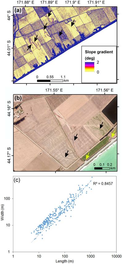
2                                                                    A. Micallef et al.: Groundwater erosion of coastal gullies

1     Introduction                                                 age has been shown to unambiguously lead to channel for-
                                                                   mation in unconsolidated sand- to gravel-sized sediments
1.1    Coastal gullies                                             (Lapotre and Lamb, 2018; Dunne, 1990), e.g. gravel-braided
                                                                   river deposits in Alaska (Sunderlin et al., 2014) and the Can-
Gullies can be incised into coastal cliffs and bluffs in a vari-   terbury Plains (Schumm and Phillips, 1986), conglomerates
ety of geologic settings around the world, owing their forma-      in the Kalahari (Nash et al., 1994), outwash and alluvial
tion to a complex interaction of hydrologic, lithospheric, tec-    sands in Florida (Schumm et al., 1995), Martha’s Vineyard
tonic and atmospheric processes. While much research has           (Uchupi and Oldale, 1994) and Vocorocas (Coelho Netto et
focused on gully formation and evolution in non-coastal set-       al., 1988), dune sand and tephra in South Taranaki (Pillans,
tings in response to changes, such as land cover and use, nat-     1985), and granodiorite regolith in the Obara area of Japan
ural hazards and/or changes in precipitation, relatively little    (Onda, 1994). In sediments finer than sands, erosion is typi-
work has focused on gully geomorphology and morphody-              cally limited by detachment of the grains at the seepage face.
namics in coastal cliffs and bluffs. The most commonly ac-         In silts and clays, the permeability is so low that the ground-
cepted mechanism for coastal gully formation is through con-       water discharge is often less than that required to overcome
centrated overland flow and knick point migration (Ye et al.,      the cohesive forces of the grains (Dunne, 1990). The role of
2013; Leyland and Darby, 2008, 2009; Mackey et al., 2014;          groundwater seepage and channel formation in bedrock, on
Limber and Barnard, 2018). Changes in land cover and use           the other hand, remains controversial (Lamb et al., 2006; Pel-
due to agriculture, logging, forest fires and other factors can    letier and Baker, 2011).
decrease surface roughness and increase concentrated over-            Our understanding of channel evolution by groundwater
land flow, which, given sufficient energy and/or time, can         seepage is predominantly derived from theoretical, experi-
erode a narrow section of coastal cliff and form a knick point.    mental and numerical models (Howard, 1995; Lobkovsky et
Depending on the resistive forces (e.g. geology and uplift)        al., 2004; Chu-Agor et al., 2008; Wilson et al., 2007; Petroff
relative to the erosive force of the overland flow, this knick     et al., 2011; Pelletier and Baker, 2011; Higgins, 1982). Such
point will migrate inland over time, incising a gully into the     studies suggest that the velocity at which channel heads ad-
cliff or bluff. Recent work has focused on modelling coastal       vance is a function of the groundwater flux and the capac-
gully formation and evolution as knick point migration (Lim-       ity of seepage water to transport sediment from the seepage
ber and Barnard, 2018).                                            face (Fox et al., 2006; Howard and McLane, 1988; Abrams
   Coastal cliff stability and gully incision can be affected by   et al., 2009; Howard, 1988), and that channel head erosion
processes of concentrated overland flow, quarrying by waves        occurs by episodic headwall slumping (Kochel et al., 1985;
at the base of the cliff and groundwater discharge (Limber         Howard, 1990). Channels incised by groundwater seepage
and Barnard, 2018; Kline et al., 2014), although it is unclear     have been shown to branch at a characteristic angle of 72◦
when and where each of these factors is important (Collins         at stream tips, which increases to 120◦ near stream junctions
and Sitar, 2009, 2011). While overland flow is a common            (Devauchelle et al., 2012; Yi et al., 2017), whereas grow-
formation mechanism, it is possible to have coastal gullies        ing indentations competing for draining groundwater results
form where the cliff is affronted by a beach, which limits the     in periodically spaced channels (Dunne, 1990; Schorghofer
basal quarrying or notching by waves, and where there is no        et al., 2004). Channel network geometry appears to be deter-
outward sign of overland flow. Relatively little attention has     mined by the external groundwater flow field rather than flow
been paid to the potentially important role of groundwater as      within the channels themselves (Devauchelle et al., 2012).
a driver of coastal gully formation and evolution, despite the        A number of fundamental questions related to the evo-
potential for groundwater to affect the geotechnical proper-       lution of channels by groundwater seepage in unconsol-
ties of coastal cliffs (Collins and Sitar, 2009, 2011).            idated sediments remain unanswered. First, the temporal
                                                                   scale at which channels form is poorly quantified due to the
1.2    Channel erosion by groundwater seepage                      paucity of process-based observations and detailed instru-
                                                                   mental analysis. Field observations of groundwater processes
Groundwater has been implicated as an important geomor-            are rare (e.g. Onda, 1994), primarily due to the difficulty with
phic agent in channel network development, both on Earth           accessing the headwalls of active channels, the potentially
and on Mars (Kochel and Piper, 1986; Higgins, 1984; Dunne,         long timescales involved and the complexity of the erosive
1990; Malin and Carr, 1999; Harrison and Grimm, 2005;              process (Dunne, 1990; Chu-Agor et al., 2008). Quantitative
Salese et al., 2019; Abotalib et al., 2016). The classic model     assessments of channel evolution have relied on experimen-
entails a channel headwall that lowers the local hydraulic         tal and numerical analyses, but these tend to be based on sim-
head and focuses groundwater flow to a seepage face. This          plistic assumptions about flow processes and hydraulic char-
leads to upstream erosion by undercutting, the rate of which       acteristics. Experimental approaches are based on a range
is limited by the capacity of seepage water to transport sed-      of different methods, limiting comparison of their outcomes
iment from the seepage face (Dunne, 1990; Howard and               (Nash, 1996). Published erosion rates vary between 2–5 cm
McLane, 1988; Abrams et al., 2009). Groundwater seep-              per century (Schumm et al., 1995; Abrams et al., 2009) and

Earth Surf. Dynam., 9, 1–18, 2021                                                       https://doi.org/10.5194/esurf-9-1-2021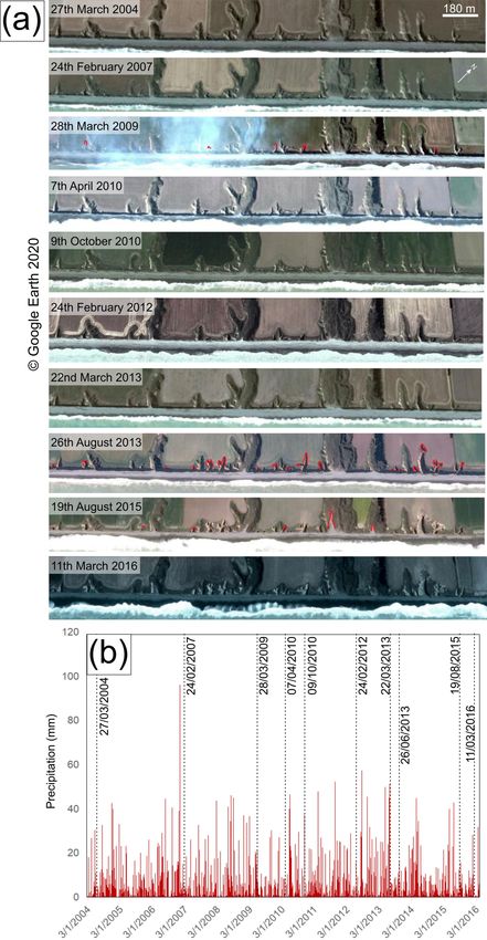
A. Micallef et al.: Groundwater erosion of coastal gullies                                                                   3

450–1600 m3 per year (Coelho Netto et al., 1988). Second,        cemented matrix-supported outwash gravel, which is capped
the influence of geologic heterogeneities on channel evolu-      by up to 1 m of post-glacial loess and modern soil (Berger
tion is also poorly understood. Lithological strength and per-   et al., 1996). The cliff face is punctuated by ∼ 0.5 m thick
meability contrasts are rarely simulated by experimental and     lenses of sand or clean gravel.
numerical analyses. Third, there are only a few places where
the mechanisms by which seepage erosion occurs have been         3     Materials and methods
clearly defined (e.g. Abrams et al., 2009). Basic observations
and measurements of channel erosion rates and substrate ge-      3.1     Data
ologic heterogeneities are needed to test and quantify models
for channel formation and improve our ability to reconstruct     3.1.1    Field visits
and predict landscape evolution by groundwater-related pro-      Site visits were carried out in May 2017 and 2019. Dur-
cesses.                                                          ing these visits, geomorphic features of interest were noted
                                                                 and photographed and samples were collected. Samples in-
1.3    Objectives                                                cluded outcropping sediment layers across the cliff face for
                                                                 grain size analyses, sediments with coating for geochemical
In this study, we revisited the Canterbury Plains study site
                                                                 analyses and loess sediments for geochronological analysis
(Schumm and Phillips, 1986) and carried out field obser-
                                                                 (NZ13A and NZ14A; Fig. 1). The latter were collected from
vations, geochronological analyses, repeated remote sensing
                                                                 the base of the loess draping the flanks of the two largest
surveys, near-surface geophysical surveying and slope stabil-
                                                                 gullies, above the boundary with the underlying gravels, by
ity modelling of coastal gullies to (i) identify the processes
                                                                 hammering stainless steel tubes into the sediment and ensur-
by which groundwater erodes gullies along the coast, (ii) as-
                                                                 ing that the material was not exposed to light.
sess the influence of geological/permeability heterogeneity
on the gully formation process and (iii) quantify the timing
of gully erosion and its key controls.                           3.1.2    Unoccupied aerial vehicle (UAV) surveys
                                                                 Unoccupied aerial vehicle (UAV) surveys were carried out
2     Regional setting                                           using DJI Phantom 4 Pro and DJI Mavic Pro drones. The
                                                                 surveys were carried out after rainfall events and on the fol-
The flat to gently inclined Canterbury Plains, located in the    lowing dates: 11 May, 19 and 30 June, 11, 15, 23 and 29 July,
eastern South Island of New Zealand, extend from sea level       4 and 26 August, 11 and 23 September, and 6, 13 and 30 Oc-
up to 400 m above sea level and cover an area of 185 km          tober 2017. The drones were flown at an altitude of 40–55 m,
by 75 km (Fig. 1a). A series of high-energy braided rivers       a speed of 5 m s−1 and side lap of 65 %–70 %. A total of
emerge from the > 3500 m high Southern Alps and flow             eight ground control points were selected, and their loca-
southeastwards to the shoreline (Kirk, 1991). The plains         tion and elevation were determined by differential GPS with
were formed by the coalescence of several alluvial fans          centimetre-scale horizontal and vertical accuracy. Orthopho-
sourced from the these rivers (Leckie, 2003; Browne and          tos and digital elevation models with a horizontal resolution
Naish, 2003). The Quaternary sedimentary sequence com-           of 10 cm per pixel were generated from the UAV data using
prises a > 600 m thick succession of cyclically stacked          DroneDeploy. The mean distance between the ground con-
fluvio-deltaic gravel, sand and mud with associated aeo-         trol points and the generated orthophoto and model grid cell
lian deposits and palaeosols (Browne and Naish, 2003; Bal,       centres was 0.03 m. Root mean square and bias were used to
1996). The gravels consist of greywacke and represent a va-      estimate the vertical accuracy of the digital elevation mod-
riety of channel-fill beds and bar forms, whereas the iso-       els (equations in Laporte-Fauret et al., 2019). The root mean
lated bodies of sand are relict bars and abandoned chan-         square error and bias were 0.05 and 0.03 m, respectively. The
nels. The interglacial sediments are better sorted and have      model elevations were slightly underestimated (0.1 m).
higher permeability than the glacial outwash, resulting in a
wide range of hydraulic conductivities (Scott, 1980). New
                                                                 3.1.3    Near-surface geophysics
Zealand’s largest groundwater resource is hosted in the grav-
els down to at least 150 m depth (Davey, 2006). The up-          Time domain electromagnetic (TEM) measurements were
per Quaternary sediments are exposed along a 70 km long          carried out in May 2019 using the Geonics (Canada) G-
coastline southwest of the Banks Peninsula (Moreton et al.,      TEM system (Fig. 1b). The operating principles of the in-
2002). This coastline is retrograding at approximately 0.5–      ductive TEM technique are described in Nabighian and Mac-
1 m yr−1 and consists of cliffs fringed by mixed gravel and      nae (1991) and Fitterman (2015). The survey parameters in-
sand beaches (Gibb, 1978). The study area is a 2.5 km long       cluded four turns, a 10 × 10 m2 square TX loop and a TX cur-
stretch of cultivated coastline located 16 km to the southeast   rent output of 1 A. The G-TEM was operated in a fixed offset
of Ashburton (Fig. 1b). The coastline within the study area      sounding configuration, which is termed “slingram” mode,
consists of a 15–20 m thick exposure of poorly sorted and un-    in which the RX coil was placed 30 m from the centre of the

https://doi.org/10.5194/esurf-9-1-2021                                                    Earth Surf. Dynam., 9, 1–18, 2021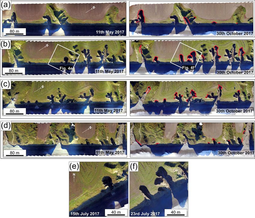
4                                                                          A. Micallef et al.: Groundwater erosion of coastal gullies

Figure 1. (a) Digital elevation model of the Canterbury Plains (source – Environment Canterbury), located along the eastern coast of the
South Island of New Zealand, showing the location of mapped gullies. The location of figure is shown in the inset. (b) Mosaic of aerial pho-
tographs of the study area (see a for location; source – Environment Canterbury). The location of luminescence dating (optically stimulated
luminescence – OSL) samples, G-TEM transects and other figures is shown. (c–d) Enlarged sections of the aerial and site photographs of the
luminescence-dating sampling sites of NZ13A and NZ14A.

TX loop and the TX–RX pair moved together along a linear                3.1.4    Other data
transect at 5 m station spacing, maintaining the 30 m offset.
                                                                        Satellite images with a horizontal resolution of 1 m per pixel
The maximum depth of investigation of the G-TEM system
                                                                        and dating back to 2004 were obtained from Google Earth.
is given approximately by the following formula:
                                                                        Precipitation records dating back to 1927 were provided by
d = 8.94L0.4 ρ 0.25 ,                                          (1)      Environment Canterbury. The latter also provided a time se-
                                                                        ries of water level data since 2015 from a 30 m deep well
where L (metres) is the TX loop size, and ρ ( m)                       located 10 km to the northeast of the study area.
is the upper layer resistivity (Geonics, 2016). Setting
ρ = 100  m yields a depth of investigation of d =71 m,                 3.2     Methods
whereas ρ = 1000 m yields d = 126 m. Our investigation
                                                                        3.2.1    Sample analyses
depth in New Zealand may be slightly greater than these val-
ues since the Geonics formula assumes a one-turn TX loop                Sediment samples were analysed for grain size distribution
carrying a current of 3 A, whereas we used a more powerful              using sieves following the American Society for Testing and
combination of four turns at 1.5 A. At each station, a con-             Materials (ASTM) D0422 protocol. The composition of the
sistent 1D smooth model of electrical resistivity vs. depth             coating on selected sediment outcrops within the gullies was
was performed based on the iterative Occam-regularised in-              determined using X-ray fluorescence.
version method (Constable et al., 1987) and using IXG-TEM
commercial software (Interpex, 2012). This is a standard 1D
                                                                        3.2.2    Luminescence dating
TDEM inversion code that has previously been successfully
used in coastal hydrogeophysical studies (e.g. Pondthai et al.,         Luminescence dating is a numerical-age technique that uses
2020).                                                                  optically and thermally sensitive signals measured in the

Earth Surf. Dynam., 9, 1–18, 2021                                                              https://doi.org/10.5194/esurf-9-1-2021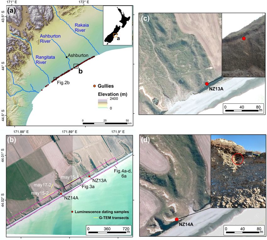
A. Micallef et al.: Groundwater erosion of coastal gullies                                                                       5

form of light emissions in the constituent minerals that form      factor of safety Ff is calculated using the following (Fred-
sediment deposits. Quartz and feldspars are among the most         lund and Krahn, 1977; Fredlund et al., 1981):
often used minerals. Sediment ages obtained via lumines-                 P 0
cence dating reflect the last exposure of the analysed mineral             (c β cos α + (N − uβ) tan φ 0 cos α)
                                                                   Ff =         P            P                  ,           (2)
grains to daylight, when the resetting (called bleaching) of                       N sin α − D cos ω
the previously incorporated luminescence signal occurs.
   In order to obtain luminescence ages, two types of mea-         where c0 (in kilopascal) is the effective cohesion, φ 0 (in de-
surements were performed. The dose accrued by the crystal          grees) is the effective angle of friction, u (in kilopascal) is
from natural radioactivity since its last exposure to daylight     pore water pressure, D (in kilonewtons) is the concentrated
(called the palaeodose) was determined as an equivalent dose       point load, β (in metres) represents the slice base length, ω
(De ). This was done by measuring the light emission of the        (in degrees) is the angle between the top part of the slope and
crystal upon optical stimulation and matching this emission        surface forces, and α (in degrees) is inclination of the slice
to signals generated by the exposure to a known dose of radi-      base. N is the normal force acting on the slice base and can
ation given in the laboratory. This is expressed as the amount     be computed by the following:
of absorbed energy per mass of mineral (1 J kg−1 = 1 Gy –
                                                                   N = W cos α − kW sin α + [D cos (ω + α − 90)],              (3)
Gray). Radioactivity measurements were carried out on each
sample in order to determine the annual dose (Da ), which
                                                                   where W (in kilonewtons) is the slice weight (unit weight
represents the rate at which the environmental dose was de-
                                                                   γs (in kilonewtons per cubic metre) × volume (in cubic me-
livered to the sample (Gy ka−1 ). The age was obtained by di-
                                                                   tres)), and k is the hydraulic conductivity (in metres per sec-
viding the two determined parameters. As low luminescence
                                                                   ond).
sensitivity and poor dosimetric characteristics were reported
                                                                      We also modelled the groundwater flow and pore pressure
for quartz from sediments in New Zealand (see Preusser et
                                                                   distribution within the soil using the Poisson equation, which
al., 2009, and the references cited therein), we have used sig-
                                                                   is the generalised form of the Laplace equation (Whitaker,
nals from feldspars by the application of infrared stimula-
                                                                   1986) as follows:
tion based on the post-IR-IRSL225 (Buylaert et al., 2009) and
post-IR-IRSL290 (Thiel et al., 2011) protocols on polymin-              ∂ 2h       ∂ 2h
eralic fine (4–11 µm) grains as well as coarse (63–90 µm)          kx        + k y      = q,                                   (4)
                                                                        ∂x 2       ∂y 2
potassium feldspars.
   A detailed description of luminescence-dating methodol-         where q is the total discharge (in cubic metres per second), kx
ogy, including sample preparation, equivalent dose deter-          and ky are equal to the hydraulic conductivity (in metres per
mination, annual dose determination, luminescence proper-          second) in the horizontal and vertical directions, respectively,
ties (including residual doses, dose recovery tests and fading     and h is the hydraulic head (in metres).
tests), is presented in the Supplement.                               Equation (4) applies to water flow under steady-state and
                                                                   homogeneous conditions, whereas the following equation is
3.2.3   Morphological change detection                             applicable to dynamic and inhomogeneous conditions:

The method used to measure gully aerial erosion in between          ∂      ∂h       ∂       ∂h          ∂θ
                                                                        kx      +        ky      =q+ ,                          (5)
surveys entailed the manual delineation of shapefiles around       ∂x      ∂x      ∂y       ∂y          ∂t
gully boundaries for each survey (using orthophotos, digital
elevation models and slope gradient maps, in the case of the       where ∂θ/∂t describes how the volumetric water content
UAV data, and satellite images, in the case of the Google          changes over the time.
Earth data), the estimation of their areas and the compari-          The water transfer theory accounts for transient behaviour,
son of the latter in between surveys. The uncertainty inher-       which can be defined by the following equation (Domenico
ent in this approach is related to the digitisation of the gully   and Schwartz, 1997):
boundaries. We made sure that a vertex was added at least
                                                                            dMst
every 5 pixels for both the UAV (0.5 m) and Google Earth           Mst =         = min − mout + Ms ,                           (6)
data (5 m). This ensures that a minimum erosion of 0.25 m2                   dt
(in the case of the UAV data) and 25 m2 (in the case of the        where min is the cumulative mass of water that enters the
Google Earth data) was detected.                                   porous medium, mout is equal to the mass of water that leaves
                                                                   the porous medium, and Ms is the mass source within the
3.2.4   Slope stability modelling                                  representative elementary volume. The rate of increase in the
                                                                   mass of water stored within the representative elementary
We developed a slope stability model based on the limit equi-      volume is as follows:
librium and segmentation strategy of the Bishop method,
whereby a soil mass is discretised into vertical slices. The       Mst = Mw + Mv ,                                             (7)

https://doi.org/10.5194/esurf-9-1-2021                                                         Earth Surf. Dynam., 9, 1–18, 2021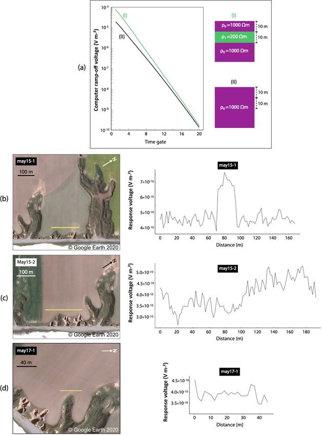
6                                                                    A. Micallef et al.: Groundwater erosion of coastal gullies

where Mw and Mv represent the rate of change in liquid wa-
ter and water vapour, respectively.
   The relationship between water level and changes in pore
water pressure can be expressed by the following:

u = ρw ghw ,                                                (8)

where ρw is the water density, and hw is the height of the
water column.
   Changes in vertical stress due to changes in pore water
pressure can be represented by the pore water pressure coef-
ficient B (Skempton, 1954), which is defined as follows:

B = 1u/1σ1 ,                                                (9)

where 1σ1 is the change in the major principal stress, which
is often assumed, for simplicity, to be equal to the change in
vertical stress (σ v). The coefficient then becomes the follow-
ing:

B = 1u/1σ v.                                               (10)

B is a general way of describing pore water conditions in a
slope stability analysis.
   The mechanical and hydraulic soil properties employed in
this model are listed in Table 1 and were obtained from Dann
et al. (2009) and Aqualinc Research Limited (2007). We
modelled two scenarios based on the available rainfall data
(see Sect. 4.4). The first is a 3 d long intense rainfall event
((I-D)3 ) covering the period 20–22 July 2017. The second is
a 14 d period with occasional, low-intensity rain ((I-D)14 ) be-
tween 21 June and 4 July 2017. Each scenario is modelled for
two sandy gravel slopes with different permeabilities – one
with a 0.5 m thick sand lens and the other with a 0.5 m thick
gravel lens. Both lenses are located at a height of 5 m above
sea level. Lateral water inflow and surface water infiltration
were estimated from the hydrological model in Micallef et
al. (2020). Slope stability modelling and groundwater anal-
yses were carried out using the Slide2 software package by
Rocscience.

4     Results

4.1    Gullies along the Canterbury coast – distribution
       and morphology
We have mapped 315 gullies (locally also known as dongas)
along 70 km of the Canterbury coastline (mean of 4.5 gullies
per square kilometre of coastline). The spatial distribution       Figure 2. (a) Slope gradient map of the study area. Black arrows in-
of the gullies is clustered (nearest-neighbour ratio of 0.33,      dicate relict infilled channels. (b) Aerial photograph of Coldstream
with a z score of −22.67 and a p value of 0); the majority         on the Canterbury coast (source – Environment Canterbury). Black
of the gullies are located between the Rakaia and Rangitata        arrows indicate relict infilled channels. Yellow arrows indicate gul-
rivers (Fig. 1a), particularly in the vicinity of the Ashburton    lies. Location shown in Fig. 1a. (c) Plot of length vs. width for gul-
River. The heads of many gullies connect to shallow, relict        lies mapped along the Canterbury coastline.
meandering channels (Fig. 2a). Some of these channels are
visible in aerial photographs, in spite of the terrain having
been worked by farmers (Fig. 2b).

Earth Surf. Dynam., 9, 1–18, 2021                                                         https://doi.org/10.5194/esurf-9-1-2021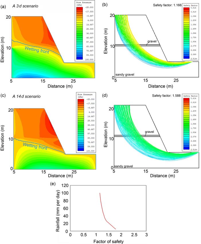
A. Micallef et al.: Groundwater erosion of coastal gullies 7
Table 1. Mechanical and hydraulic soil properties used in slope stability modelling.
Soil type Unit weight Cohesion Friction Saturated hydraulic Residual water content Saturated water content
(kN m−3 ) (kPa) angle (◦ ) conductivity (m3 m−3 ) (m3 m−3 )
(m d−1 )
γs c ϕ k θr θs
Sand 20.5 7 34.5 3.216 0.01 0.078
Sandy gravel 23 8 37 0.64 0.01 0.128
Gravel 24 4 36.5 7.376 0.016 0.142
In plan view, the gullies are predominantly linear to
slightly sinuous (sinuosity of 1–1.3) and characterised by a
concave head. In profile, the gullies have linear, gently slop-
ing (2–10◦ ) axes, with a concave break of slope separating
the axis from a steep (up to 70◦ ) head. In cross section, the
gullies are U-shaped, with walls of up to 70◦ in slope gra-
dient. The gullies are between 5 and 1134 m long (mean of
116 m) and between 3 and 637 m wide (mean of 56 m). Gul-
lies generally exhibit a constant width with a distance ups-
lope. They have a length-to-width ratio that varies between
1 and 7.9, with a mean of 2 (standard deviation of 0.89;
Fig. 2c).
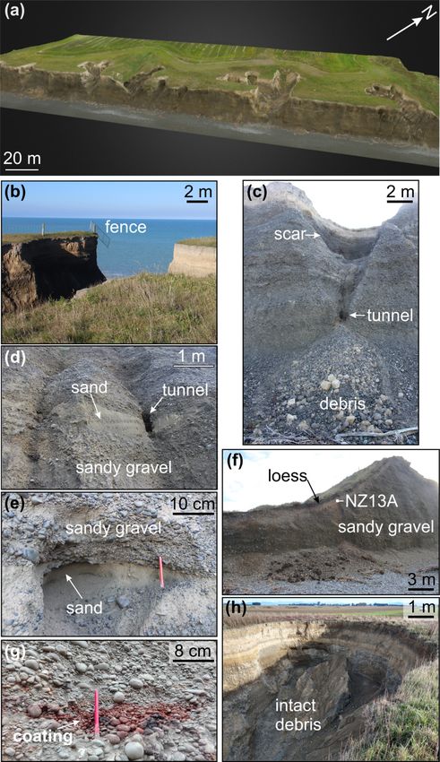
4.2 Field site observations
In May 2017, our study area hosted 33 gullies that vary be-
tween 15 and 600 m in length (Figs. 1b, 3a). During the
site visits, we did not encounter evidence of surface flow.
However, the middle to lower sections of the gully walls
and cliffs were consistently wet. These sections were also
characterised by failure scars and alcoves, particularly above
the sandy lenses. Alcoves were also encountered at the base
of gully heads, where they were wet and up to 1 m deep
(Fig. 3e). Some sandy layers outcropping across the cliff
face hosted tunnels (Fig. 3c–d). Above these tunnels, theatre-
shaped scars with a shallow and narrow gully at their base
were observed (Fig. 3c). At the base of the scars, the gully
heads and some gully mouths, we encountered mass move-
ment debris that was occasionally intact and that predomi-
nantly consisted of gravel, sandy gravel and loess (Fig. 3c,
h). Gullies have gravel-covered irregular floors. Whereas
the smaller gullies have a U-shaped cross section, the three
longest gullies have gently sloping V-shaped cross sections,
with loess draping their walls (Fig. 3f). Sandy and clean
gravel layers outcropping within the gullies were wet; the
former appeared weathered, whereas the latter were coated
by Fe and Mn (Fig. 3g). Fences were locally seen suspended
across a number of gullies (Fig. 3b).
Figure 3. (a) Orthophoto map of part of the study area draped on a
3D digital elevation model. Location shown in Fig. 1b. (b–h) Pho-
tographs of features of geomorphic interest taken at the study area.
The location of sample NZ13A is shown in (f).
https://doi.org/10.5194/esurf-9-1-2021 Earth Surf. Dynam., 9, 1–18, 2021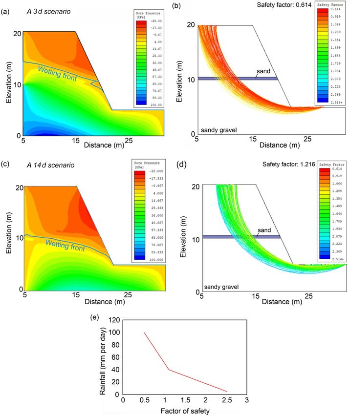
8                                                                   A. Micallef et al.: Groundwater erosion of coastal gullies

4.3     Infrared stimulated luminescence ages                     a major rainfall event between 16 and 23 June 2013, when
                                                                  171 mm of rain fell in 7 d (with up to 51 mm falling in 1 d;
Four sets of infrared stimulated luminescence ages are pre-       Fig. 6b). The other erosion episodes include the five gullies
sented in Table 2. The pIRIR290 ages are higher than the ages     eroded by 28 March 2009, after a storm of 46 mm d−1 on
obtained by applying the pIRIR225 protocol. The cause of          31 July 2008, and the five gullies eroded by 19 October 2015,
this difference is not yet fully understood, although it can      after a storm of 43 mm d−1 on 19 June 2015.
partially be attributed to the results of the dose recovery
test and the poor bleachability of the pIRIR290 signals com-
pared to pIRIR225 signals (Buylaert et al., 2011). Consider-      4.5   Geophysical data
ing that no anomalous behaviour of the investigated signals       The location of the G-TEM transects is shown in Fig. 1b. An
was observed (see the Supplement), we are unable to explain       attempt was made to invert the G-TEM slingram-mode re-
the overestimation of the K-feldspar ages compared to the         sponses with 30 m TX–RX offset, using a 1D Occam inver-
polymineralic fine-grain ages in the case of NZ13A, espe-         sion. A representative inversion result is shown in Fig. 7. The
cially since the opposite behaviour is observed in the case       resistivity model is presented in Fig. 7b, whereas the corre-
of sample NZ14A. However, considering a 95 % confidence           sponding model response with the actual data points is shown
level, infrared-stimulated luminescence ages obtained using       in Fig. 7a. The best-calculated smooth depth profile clearly
different methods broadly overlap, with the only exception        does not fit well with the measured signal, and there is exces-
being the pIRIR225 ages obtained on K-feldspars on sample         sive structure in the ∼ 10–20 m depth range, including the
NZ14A, which we regard as an outlier.                             very low resistivity layer (∼ 10−4 m) at depths in excess
                                                                  of ∼ 12–15 m. The resistivity values between 40 and 100 m
4.4     Morphological changes                                     depth are lower than sea water resistivity (0.3 m), which is
                                                                  not reasonable. The inability to fit a 1D model to the slingram
4.4.1    Short-term morphological changes
                                                                  responses suggests that the geoelectrical subsurface structure
By comparing the orthophotos and digital elevation models         is strongly heterogeneous within the footprint of the G-TEM
generated from the UAV data acquired during the various site      transmitter. As a result, we cannot trust 1D inversions of the
visits between May and October 2017, we document the for-         slingram-mode data in such a 3D geological environment.
mation of three new gullies (up to 30 m long; Figs. 4e–f)         We did not try to use the 1D inversion software to further
and the enlargement of 30 gullies (primarily by elongation        analyse and interpret the G-TEM data. However, even though
and occasionally by widening and branching; Fig. 4a–d). The       the individual slingram-mode responses cannot be fitted reli-
new gullies formed at locations where there was a small land-     ably by a 1D model, we can still analyse the lateral changes
slide scar in the middle of the cliff. There was no change in     in the observed response curves along the slingram profiles
form in three of the gullies. Figure 5 shows the total area       to reveal information about subsurface heterogeneity; this is
eroded between surveys (which amounts to approximately            elaborated on below.
3273 m2 ), the daily precipitation and the associated changes        Instead of performing 1D inversions, we present time gate
in water table height. Only three surveys recorded gully ero-     plots for all three transects. A time gate plot is defined as a
sion. A total of two of these surveys happened soon after         graph of the observed G-TEM voltage response, evaluated at
rainfall events of > 40 mm in 1 d (Fig. 5). The most impor-       a particular time gate, as a function of a position along a pro-
tant of these covers the period between 15 and 23 July 2017       file. Time gate plots are a useful alternative for exploring the
when 95 % of the material was removed and the three new           lateral variability in the G-TEM response along a profile in
gullies were formed (Figs. 4–5). During this period, a total      the event that the sounding curves at individual stations can-
of 153 mm of rain fell (up to 120 mm on 21 July 2017 alone,       not be fitted with 1D models. It is presumed that the variabil-
which was the most intense rainfall event since 1936), result-    ity in a time gate plot is correlated with lateral heterogeneity
ing in a 1.5 m rise in the water table. A third survey occurred   in the subsurface geoelectrical structure, since a 1D Earth
6 d after the 21 July 2017 storm, with 22 mm of rain falling      structure would yield no spatial variability in a time gate
in 1 d. The material eroded from the gullies was deposited at     plot. In general, due to lengthy signal-averaging times, ambi-
the base of the cliffs as gravel cones, which were remodelled     ent electromagnetic noise from the environment adds a very
by debris flows during the ensuing precipitation events and       small contribution to TDEM responses, such that any along-
subsequently disappeared from the orthophotos.                    profile variations are likely caused by geological heterogene-
                                                                  ity. However, there is not a straightforward relationship be-
4.4.2    Long-term morphological changes
                                                                  tween the magnitude of the TDEM voltage at any given time
                                                                  gate and the resistivity within a particular subsurface volume.
For the period 2004–2015, we used satellite imagery to map        The situation becomes more complicated since the true Earth
the formation of six new gullies and the elongation of 22         is characterised by multiscale heterogeneity, such that spa-
gullies. A total of 18 of these erosion episodes are recorded     tial variations in the geology at all length scales superimpose
in the image taken on 26 August 2013 (Fig. 6a). This follows      their individual responses on one another to produce the final

Earth Surf. Dynam., 9, 1–18, 2021                                                      https://doi.org/10.5194/esurf-9-1-2021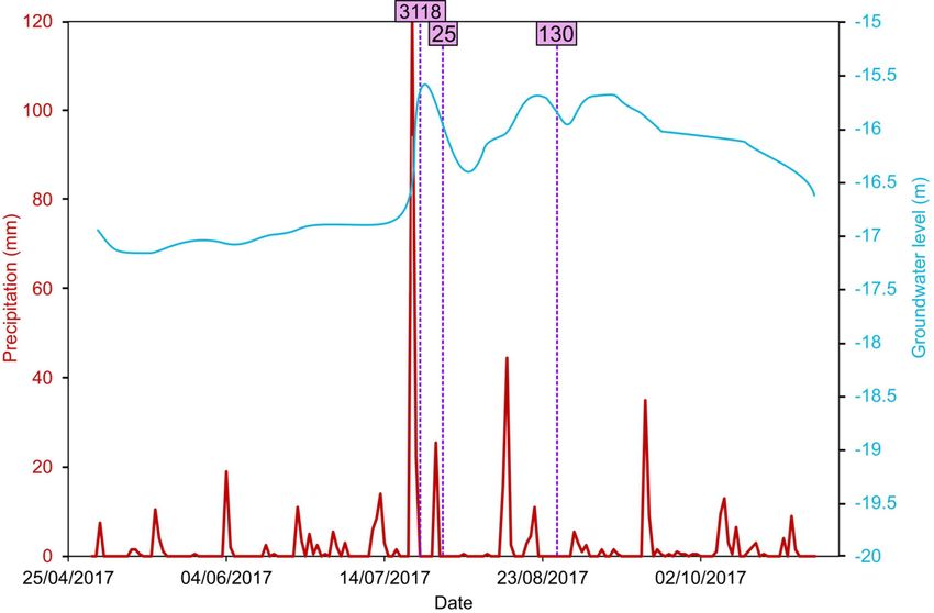
A. Micallef et al.: Groundwater erosion of coastal gullies                                                                              9

Table 2. Summary of the pIRIR225 and pIRIR290 ages obtained on polymineralic fine grains (4–11 µm) and coarse K-feldspars (63–90 µm).
The infrared stimulated luminescence ages were determined considering 15 % water content. Uncertainties are given at 1σ , with a 68 %
confidence level. Further details are available in the Supplement.

                                                   Age (ka) pIRIR225                 Age (ka) pIRIR290
                            Sample code     Polymineralic fine   K-feldspars    Polymineralic    K-feldspars
                                                       grains    (63–90 µm)        fine grains   (63–90 µm)
                            NZ13A                   16.0 ± 1.4     20.1 ± 1.5       20.9 ± 2.0     26.2 ± 2.1
                            NZ14A                    4.6 ± 0.4      1.9 ± 0.1        6.0 ± 0.7      3.1 ± 0.3

Figure 4. (a–d) Orthophotographs of the study area at the start and end of the UAV surveys, ordered from southwest to northeast. Red lines
mark eroded areas. Location shown in Fig. 1b. Orthophotographs from a part of the study area on (e) 15 July 2017 and (f) 23 July 2017.
Location shown in (b).

https://doi.org/10.5194/esurf-9-1-2021                                                            Earth Surf. Dynam., 9, 1–18, 2021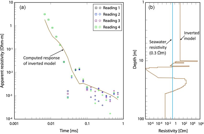
10                                                                        A. Micallef et al.: Groundwater erosion of coastal gullies

Figure 5. Daily precipitation (for Ashburton District Council) and
groundwater level records (from a well located 10 km northeast of
the study area) for the period 1 May to 31 October 2017 (source –
Environment Canterbury). The pink lines mark the surveys during
which gully erosion was observed (the value in the pink box corre-
sponds to the eroded area in square metres; uncertainty is 0.25 m2 ).

overall TDEM response that is measured. Thus, any analy-
sis of the spatial variability in a time gate plot, while infor-
mative, is largely qualitative and indicates only a first-order
spatial distribution of causative subsurface structures.
   Specifically, the amplitude of the G-TEM slingram re-
sponse (in units of 10−10 V m−2 ) at the first time gate is plot-
ted as a function of the station number along a profile. Fig-
ure 8a displays a 1D model (I) that contains a conductive
layer of 200 m between a 10 and 20 m depth in a homoge-
neous 1000 m background. The 1D model (i) is motivated
by the inversion results of deep-penetrating 40 × 40 m TX
loop TDEM soundings carried out on top of the cliffs several
tens of metres inland (Weymer et al., 2020), which revealed
such a conductive zone at these depths. Unlike the slingram
profiles, the deeper-penetrating, larger-loop sounding curves
are readily fitted by a 1D model. This model generates a G-
TEM slingram response that has a substantially larger ramp-
off voltage amplitude at all time gates than the model does
(ii) without the conductive layer, as shown in Fig. 8a. Thus,           Figure 6. (a) Satellite imagery of the study area between the
we regard an enhancement in the response at the first time              27 March 2004 and 11 March 2016 (source – © Google; Maxar
gate as indicative of a conductive zone at depth beneath the            Technologies). Eroded areas are marked by red lines. (b) Daily
                                                                        precipitation record for this period for Ashburton District Council
slingram station. The spatial analysis of the time gate plots is
                                                                        (source – Environment Canterbury). The dates on which the satellite
not a conventional approach in time domain electromagnet-               imagery was collected are denoted.
ics, but it is somewhat analogous to the spatial analysis of the
apparent resistivity profiles in frequency domain electromag-
netics using terrain conductivity meters (e.g. Weymer et al.,
2016). This is based on the idea that the G-TEM response at a           at time gate number 1, which is the first sampled point of the
fixed time gate carries information similar to that of a terrain        transient response immediately after the TX current has been
conductivity meter response at a fixed frequency.                       switched off. Near the middle of this transect, there is a dis-
   The first time gate profile of transect May15-1 is located           tinctive peak that is much higher than the background. The
upslope of small but recently eroded gullies (Fig. 8b). In this         peak is ∼ 20–30 m wide, and it appears in a similar fashion
figure, the first time gate profile is a plot as a function of the      on each of the gates 1 through 7 (not shown here), although
distance along the transect of the G-TEM ramp-off voltage               it cannot be clearly observed after gate 7. Transect May15-2

Earth Surf. Dynam., 9, 1–18, 2021                                                             https://doi.org/10.5194/esurf-9-1-2021
A. Micallef et al.: Groundwater erosion of coastal gullies 11
Figure 7. A 1D inversion result for G-TEM data, shown as squares and diamonds (representing positive and negative responses, respectively),
at a station located 6 m from start of profile May15-1. (a) The computed resistivity depth profile displayed as a curve passing through data
points. (b) The best-fit model is marked as the brown line, while the light blue line is the inferred seawater resistivity.
is located upslope of recently eroded gullies in the southwest associated to high pore pressures within the sand lens, and
and relatively less active gullies in the northeast of the inves- then to 0.614, as a result of a decrease in the shear strength
tigated area (Fig. 8c). Lateral variations are evident along the of the lower slope material due to an increase in pore pressure
192 m length of the profile. The high-amplitude response at (Fig. 9a–b). A rainfall intensity of 40 mm d−1 is required to
the start of the profile (going from the southwest to the north- bring the factor of safety below 1 (Fig. 9e), and up to 4.4 m3
east) is followed by a drop in amplitude near the midpoint of of water is estimated to have seeped out of the cliff face to
the profile, after which there is continuous fluctuation at a erode 1650 m3 of material. In the case of the second scenario
lower amplitude until the end of the profile. The time gate ((I-D)14 ), changes in pore water pressure did not result in
plots for gates 2 to 7 remain similar in shape to that of the either tunnelling or slope failure. This only resulted in a de-
time gate 1 plot and, hence, are not shown. After time gate 7, crease in the effective stress and in the factor of safety (1.216;
the time gate plots start to lose coherence due to the low Fig. 9c–d).
signal-to-noise ratio of the decaying RX voltage at late times
after TX ramp off. The G-TEM slingram profile May17-2
4.6.2 Slope with gravel lens
was acquired upslope of the tributary of a large gully cov-
ered by mature vegetation (Fig. 8d). As shown in Sect. 4.4, The factor of safety of the slope prior to any rainfall event
the size and location of this gully have been persistent over is 1.793. For the first scenario ((I-D)3 ), the factor of safety
recent years, in contrast to the neighbouring, smaller gullies decreased to 1.166, and neither tunnelling nor slope failure
that are under active development. Transect May17-2 shows occurred (Fig. 10a–b). In the case of the second scenario ((I-
a lower amplitude response in comparison to the previous D)14 ), the outcome is the same, with the factor of safety de-
two transects (Fig. 8). creasing to just 1.588 (Fig. 10c–d). The factor of safety does
Based on all three profiles, a general observation that can not reach a value lower than 1 for rainfall intensities of up to
be made is that the first time gate amplitude of the slingram 120 mm d−1 (Fig. 10e).
response is higher upslope of the more recently active gullies.
5 Discussion
4.6 Slope stability modelling
4.6.1 Slope with sand lens
Gullies are characteristic landforms along the Canterbury
coast (Fig. 1a). They are an important driver of coastal geo-
The factor of safety of the slope prior to any rainfall event morphic change and loss in agricultural land. In the following
was 2.514. During the first scenario ((I-D)3 ), the factor of sections, we integrate field observations with the modelling
safety decreased to 1.371, due to undermining by tunnelling results to infer how coastal gullies are formed by groundwa-
https://doi.org/10.5194/esurf-9-1-2021 Earth Surf. Dynam., 9, 1–18, 202112 A. Micallef et al.: Groundwater erosion of coastal gullies
Figure 8. (a) G-TEM slingram response for an electrical model (I), containing a conductive zone at a depth of 10–20 m, and for a model
(II), without the conductive zone. First time gate profiles of G-TEM slingram transects of (b) May15-1, (c) May 15-2 and (d) May17-2 are
shown. The yellow line marks a slingram transect, the length of which can be determined from the scale bar. Source of background imagery
– © Google; Maxar Technologies.
ter erosion, the role that lithology and permeability play in 5.1 Coastal gully formation by groundwater-related
gully initiation and evolution and the temporal scale of gully processes
formation.
The Canterbury gullies initiate and evolve via two types of
groundwater-related processes. The first process is the seep-
age erosion of sand, which leads to the formation of alcoves
and tunnels. This inference is based on the exclusive occur-
Earth Surf. Dynam., 9, 1–18, 2021 https://doi.org/10.5194/esurf-9-1-2021A. Micallef et al.: Groundwater erosion of coastal gullies 13 Figure 9. Model results for a sandy gravel slope with a sand lens. Estimated pore water pressure and factor of safety after 3 d for the first scenario ((I-D)3 ) (a–b) and 14 d for the second scenario ((I-D)14 ) (c–d). (e) Plot of rainfall intensity vs. factor of safety for the for first scenario ((I-D)3 ) for the slope with sand lens. The results shown are for the end of the simulation for each scenario. rence of tunnels in sandy layers at the study site (Fig. 3c– ure, which results in the elongation of the gullies and, to a e). Seepage erosion lowers the overall factor of safety of the lesser extent, widening and branching along the gully walls. slope, as demonstrated by slope stability model results for the According to the slope stability model in Fig. 9a, up to 4.4 m3 slope with sand lens scenario, and is a precursor to the second of seepage water is required to erode 1650 m3 of sediments, process, which is slope failure (Fig. 3c). Site observations which contrasts with the inference by Howard (1988) that (Fig. 3h), the UAV data (Fig. 4) and satellite imagery (Fig. 5) 100–1000 times more water than volume of eroded sediment show that gullies primarily evolve by retrogressive slope fail- must be discharged in order to create a sapping valley. We https://doi.org/10.5194/esurf-9-1-2021 Earth Surf. Dynam., 9, 1–18, 2021
14                                                                           A. Micallef et al.: Groundwater erosion of coastal gullies

Figure 10. Model results for sandy gravel slope with gravel lens. Estimated pore water pressure and factor of safety after 3 d for the first
scenario ((I-D)3 ) (a–b) and 14 d for the second scenario ((I-D)14 ) (c–d). (e) Plot of rainfall intensity vs. factor of safety for the for first
scenario ((I-D)3 . The results shown are for the end of the simulation for each scenario.

infer that wave erosion is responsible for the removal of the              5.2   Influence of geological/permeability heterogeneity
failed material at the gully mouths and the base of the cliff.                   on gully formation
Isotropic scaling of length with width (Fig. 2c) suggests that
gully planform shape is generally geometrically similar at                 Two factors control the location of gullies. The first factor is
consecutive stages of evolution.                                           the occurrence of sand lenses across a sandy gravel cliff face.
                                                                           This geological framework is conducive to alcove formation,

Earth Surf. Dynam., 9, 1–18, 2021                                                                  https://doi.org/10.5194/esurf-9-1-2021
A. Micallef et al.: Groundwater erosion of coastal gullies 15
tunnelling and slope failure (Fig. 3c–e). The higher perme- 5.3 Temporal scale of gully formation
ability of the sand and clean gravel lenses, in comparison to
the surrounding sandy gravel (Table 1), facilitates faster wa- Morphological changes derived from the time series of UAV
ter transfer to the cliff face; this is also corroborated by the data (Figs. 4–5) and satellite imagery (Fig. 6), and the ob-
weathering in the sandy layers and Fe and Mn deposits in the servations of suspended fences across gullies (Fig. 3b), sug-
clean gravel layers (Fig. 3g). Alcoves and tunnels only form gest that gully formation is rapid (on daily timescales) and
in the sand lenses; however, the latter develop higher pore recent (< 3 years ago). It is an episodic process that occurs
pressures, and sand is easier to entrain and remove in com- after a threshold is exceeded. This threshold entails a rain-
parison to clean gravel in view of its lower shear strength fall intensity of > 40 mm d−1 , which occurs once every 227 d
(Table 1). Slope failure only occurs in sandy gravel slopes on average. The threshold value is based on UAV and satel-
with sand lenses (Figs. 9–10). The higher pore pressure de- lite imagery observations, which show that gullies form af-
veloped in the sand lenses is transferred to the sandy gravel ter rainfall events, with an intensity higher than 40 mm d−1
slopes, resulting in a larger decrease in the shear strength and (Figs. 5, 6), and the plot of the factor of safety with rainfall
higher water table in comparison to the sandy gravel slope intensity from the slope stability model for the first scenario
with gravel lens. ((I-D)3 for the slope with sand lens (Fig. 9). The erosion rate
The second factor is a hydraulically conductive zone ups- documented in our study area is up to 30 m d−1 (Fig. 4e-f),
lope of the gully. This inference is supported by the following which is the highest rate documented for gullies formed by
observations: (i) braided river channel infills, which tend to groundwater so far.
comprise highly permeable, coarse-grained materials (More- The majority of the gullies in our study area have shown
ton et al., 2002), lead into the gullies’ heads (Fig. 2a–b); evidence of erosion in the past 11 years (Figs. 4, 6). The
(ii) clustered distribution of gullies between the two braided luminescence-dating results (Table 2), however, suggest that
rivers with the highest flow rates (Rakaia and Rangitata the two largest gullies have largely been inactive during at
rivers; Environment Canterbury, 2019; Fig. 1a); (iii) geo- least the last 2 ka; recent erosion is only documented in
physical observations (Fig. 8). With regards to the G-TEM small gullies located in the central section of their mouths
slingram time gate plots (Fig. 8), we interpret the higher- (Figs. 4, 6). This contrasts with the inference by Schumm and
amplitude responses on the time gate 1 plots that are pref- Phillips (1986) that they were formed by the spillage of water
erentially located upslope of recently active gullies as being from swamps behind the cliffs in the 19th century. We there-
zones of relatively high electrical conductivity in the sub- fore propose that the short gullies (< 200 m in length) are
surface at depths of ∼ 10 m. These zones are suggestive of recently active features, whereas the largest gullies are relict
buried groundwater conduits made up of gravel and/or sandy features that formed as a result of higher groundwater flow,
units (Weymer et al., 2020) or tunnels formed by subsurface and possibly surface erosion, in the past. The age of sam-
groundwater flow in sand units. Further analysis of the G- ple NZ13A suggests that this may have occurred during the
TEM data, including 2D modelling and inversion, is required Last Glacial Maximum. Such a difference in age, and pos-
to ascertain the subsurface hydraulic geometry responsible sibly formation process, between gullies of different lengths
for the along-profile amplitude variations. This is elaborated may explain the different cross sectional shape and higher
on in the Supplement. The above observations confirm the scatter in the plot of length vs. width for the longer gullies
importance of spatial variations in hydrogeological proper- (Fig. 2c).
ties as a factor controlling the location of a gully. This had
initially been suggested by Dunne (1990) and has been doc- 6 Conclusions
umented for gullies in bedrock environments (Laity and Ma-
lin, 1985; Newell, 1970). Development of gullies downslope Gully erosion is a prevalent process shaping the Canterbury
of permeable conduits may also explain why most of the ero- coast of the South Island of New Zealand. In this study,
sion entails the elongation of existing gullies rather than for- we have integrated field observations, luminescence dating,
mation of new ones (Figs. 4, 6). It also agrees with the re- multi-temporal UAV and satellite data, time domain elec-
sults of the experimental modelling by Berhanu et al. (2012), tromagnetic surveying and slope stability modelling to con-
which suggest that channels grow preferentially at their tip strain the controlling factors and temporal scales of gully
when the groundwater flow is driven by an upstream flow. formation. Our results indicate that gully development in
If seaward-directed groundwater conduits are responsible for sandy gravel cliffs is a groundwater-related, episodic process
the location of gullies, the G-TEM results predict that, along that occurs when rain falls at intensities of > 40 mm d−1 .
the Canterbury coast, we should generally observe active At the study area, such rainfall events occur at a mean fre-
gully development downslope of peaks in slingram time gate quency of once every 227 d. Gullies have been developing,
plots. If this is the case, G-TEM could be used to identify the primarily by elongation, in the last 11 years, with the lat-
locations of incipient and even future gully development. est episode dating to 3 years ago. Gullies form within days,
and erosion rates can reach values of up to 30 m d−1 . Gul-
lies longer than 200 m, on the other hand, appear to be relict
https://doi.org/10.5194/esurf-9-1-2021 Earth Surf. Dynam., 9, 1–18, 202116 A. Micallef et al.: Groundwater erosion of coastal gullies
features that formed by higher groundwater flow and sur- Review statement. This paper was edited by Claire Masteller and
face erosion > 2 ka ago. The key processes responsible for reviewed by two anonymous referees.
gully development are the formation of alcoves and tunnels
in sandy lenses by groundwater seepage erosion, followed
by retrogressive slope failure. The latter is a result of under-
mining and a decrease in shear strength due to excess pore References
pressure development in the lower part of the slope. The lo-
cation of the gullies is controlled by the occurrence of hy- Abotalib, A. Z., Sultan, M., and Elkadiri, R.: Groundwater pro-
draulically conductive zones, which comprise relict braided cesses in Saharan Africa: Implications for landscape evolution
river channels, and possibly tunnels, and sand lenses exposed in arid environments, Earth-Sci. Rev., 156, 108–136, 2016.
across the sandy gravel cliff. We also show that gully plan- Abrams, D. M., Lobkovsky, A. E., Petroff, A. P., Straub, K. M.,
form shape is generally geometrically similar at consecutive McElroy, B., Mohrig, D., Kudrolli, A., and Rothman, D. H.:
stages of evolution. The outcomes of our study can improve Growth laws for channel networks incised by groundwater flow,
the reconstruction and prediction of an overlooked geohazard Nat. Geosci., 2, 193–196, 2009.
along the Canterbury coastline. Aqualinc Research Limited: Canterbury groundwater model 2.
Christchurch (NZ), Aqualinc Research Limited, L07079/1, 2007.
Bal, A. A.: Valley fills and coastal cliff s buried beneath an allu-
vial plain: Evidence from variation of permeabilities in gravel
Code and data availability. We used DroneDeploy software
aquifers, Canterbury Plains, New Zealand, J. Hydrol., 35, 1–27,
(https://www.dronedeploy.com/, DroneDeploy, 2017), IXG-TEM
1996.
software (http://www.interpex.com/, Interpex, 2020) and the Slide2
Berger, G. W., Tonkin, P. J., and Pillans, B.: Thermo-luminescence
slope stability programme (https://www.rocscience.com/software/
ages of post-glacial loess, Rakaia River, South Island, New
slide2, Rocscience, 2020) in this paper. All data from this study
Zealand, Quaternary Int., 35/36, 177–182, 1996.
appear in the tables, figures, main text and the Supplement.
Berhanu, M., Petroff, A. P., Devauchelle, O., Kudrolli, A., and
Rothman, D. H.: Shape and dynamics of seepage erosion
in a horiztonal granular bed, Phys. Rev. E, 86, 041304,
Supplement. The supplement related to this article is available https://doi.org/10.1103/PhysRevE.86.041304, 2012.
online at: https://doi.org/10.5194/esurf-9-1-2021-supplement. Browne, G. H. and Naish, T. R.: Facies development and sequence
architecture of a late Quaternary fluvial-marine transition, Can-
terbury Plains and shelf, New Zealand: implications for forced
Author contributions. AM designed the study and drafted the regressive deposits, Sediment. Geol., 158, 57–86, 2003.
paper, which was revised by all co-authors. AM, RM, PP, ME, BAW Buylaert, J.-P., Murray, A. S., and Thomsen, K. J.: Testing the po-
and PW participated in the fieldwork. RM and RPT interpreted the tential of an elevated temperature IRSL signal from K-feldspar,
UAV data and satellite imagery. NS and DC carried out the slope Radio Measurements, 44, 560–565, 2009.
stability modelling. PP and ME processed the geophysical data. AA Buylaert, J. P., Thiel, C., Murray, A. S., Vandenberghe, D., Yi, S.,
and ATG were in charge of the luminescence dating. and Lu, H.: IRSL and post-IR IRSL residual doses recorded
in modern dust samples from the Chinese Loess Plateau,
Geochronometria, 38, 432–440, 2011.
Competing interests. The authors declare that they have no con- Chu-Agor, M. L., Fox, G. A., Cancienne, R. M., and Wilson, G.
flict of interest. V.: Seepage caused tension failures and erosion undercutting of
hillslopes, J. Hydrol., 359, 247–259, 2008.
Coelho Netto, A. L., Fernandes, N. F., and Edegard de Deus, C.:
Acknowledgements. We are grateful to Robbie Bennett, Gullying in the southeastern Brazilian Plateau, Bananal, SP,
Clark Fenton and Daniele Spatola for their assistance during the in: Proceedings of the Porto Alegre Symposium, Porto Alegre,
fieldwork and to Environment Canterbury for the provision of the Brazil, 11–15 December 1988, 35–42, 1988.
data. Collins, B. D. and Sitar, N.: Geotechnical properties of weakly and
moderately cemented sands in steep slopes, J. Geotech. Geoenv-
iron., 135, 1359–1366, 2009.
Collins, B. D. and Sitar, N.: Stability of steep slopes in cemented
Financial support. This project has received funding from
sands, J. Geotech. Geoenviron., 137, 43–51, 2011.
the European Research Council (ERC) under the European
Constable, S. C., Parker, R. L., and Constable, C. G.: Occam’s in-
Union’s Horizon 2020 research and innovation programme (grant
version: Apractical algorithm for generating smooth models from
nos. MARCAN 677898 and INTERTRAP 678106).
EM sounding data, Geophysics, 52, 289–300, 1987.
Dann, R., Close, M., Flinto, M., Hector, R., Barlow, H., Thomas,
The article processing charges for this open-access
S., and Francis, G.: Characterization and estimation of hydraulic
publication were covered by a Research
properties in an alluvial gravel vadose zone, Vadose Zone J., 8,
Centre of the Helmholtz Association.
651–663, 2009.
Davey, G.: Definition of the Canterbury Plains Aquifers, Environ-
ment Canterbury, UK, U06/10, 2006.
Earth Surf. Dynam., 9, 1–18, 2021 https://doi.org/10.5194/esurf-9-1-2021You can also read