PhysCap: Physically Plausible Monocular 3D Motion Capture in Real Time

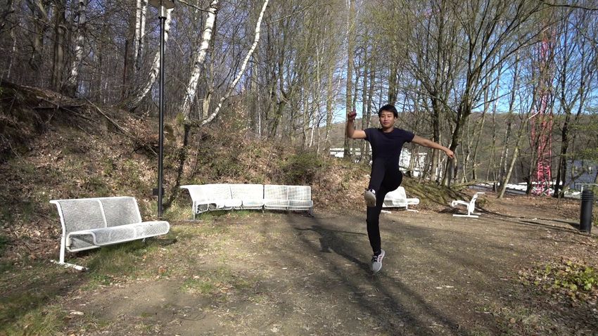
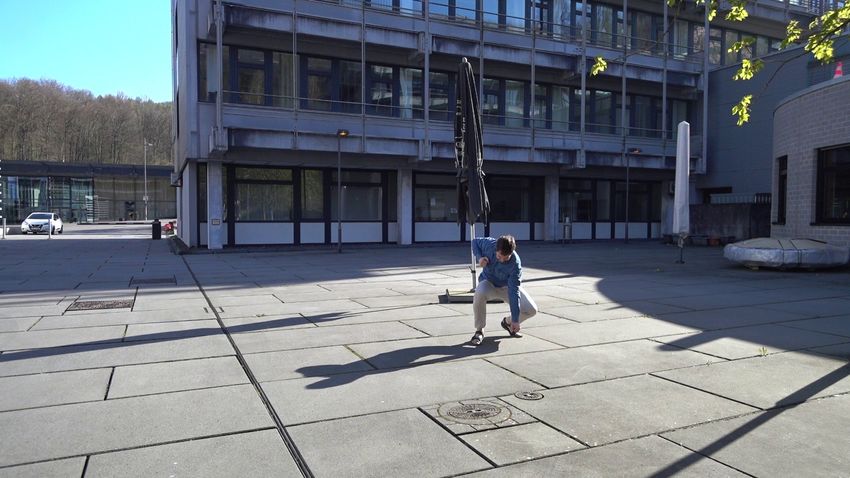
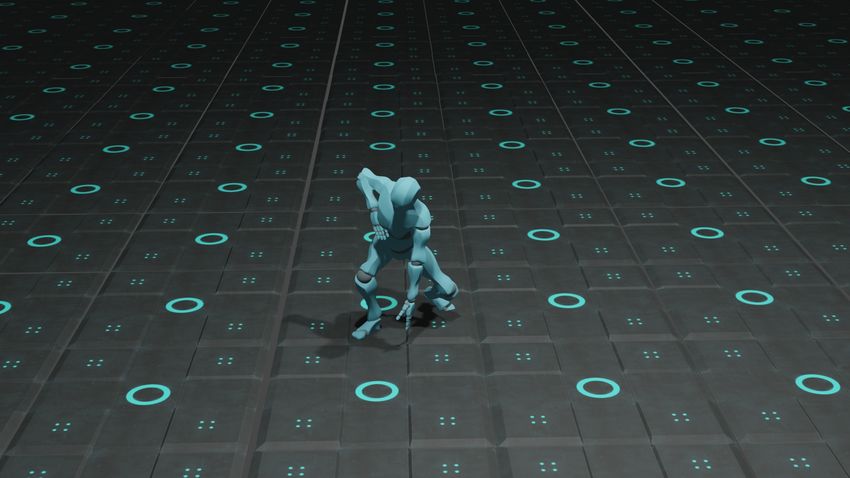
PhysCap: Physically Plausible Monocular 3D Motion Capture in Real
Time
SOSHI SHIMADA, Max Planck Institute for Informatics, Saarland Informatics Campus
VLADISLAV GOLYANIK, Max Planck Institute for Informatics, Saarland Informatics Campus
WEIPENG XU, Facebook Reality Labs
CHRISTIAN THEOBALT, Max Planck Institute for Informatics, Saarland Informatics Campus

Fig. 1. PhysCap captures global 3D human motion in a physically plausible way from monocular videos in real time, automatically and without the use of
markers. (Left:) Video of a standing long jump [Peng et al. 2018] and our 3D reconstructions. Thanks to its formulation on the basis of physics-based dynamics,
our algorithm recovers challenging 3D human motion observed in 2D while significantly mitigating artefacts such as foot sliding, foot-floor penetration,
unnatural body leaning and jitter along the depth channel that troubled earlier monocular pose estimation methods. (Right:) Since the output of PhysCap is
environment-aware and the returned root position is global, it is directly suitable for virtual character animation, without any further post-processing. The 3D
characters are taken from [Adobe 2020]. See our supplementary video for further results and visualisations.

Marker-less 3D human motion capture from a single colour camera has seen We, therefore, present PhysCap, the first algorithm for physically plau-
significant progress. However, it is a very challenging and severely ill-posed sible, real-time and marker-less human 3D motion capture with a single
problem. In consequence, even the most accurate state-of-the-art approaches colour camera at 25 fps. Our algorithm first captures 3D human poses purely
have significant limitations. Purely kinematic formulations on the basis of kinematically. To this end, a CNN infers 2D and 3D joint positions, and
individual joints or skeletons, and the frequent frame-wise reconstruction subsequently, an inverse kinematics step finds space-time coherent joint
in state-of-the-art methods greatly limit 3D accuracy and temporal stability angles and global 3D pose. Next, these kinematic reconstructions are used
compared to multi-view or marker-based motion capture. Further, captured as constraints in a real-time physics-based pose optimiser that accounts for
3D poses are often physically incorrect and biomechanically implausible, or environment constraints (e.g., collision handling and floor placement), grav-
exhibit implausible environment interactions (floor penetration, foot skating, ity, and biophysical plausibility of human postures. Our approach employs
unnatural body leaning and strong shifting in depth), which is problematic a combination of ground reaction force and residual force for plausible root
for any use case in computer graphics. control, and uses a trained neural network to detect foot contact events in im-
 ages. Our method captures physically plausible and temporally stable global
This work was funded by the ERC Consolidator Grant 4DRepLy (770784). 3D human motion, without physically implausible postures, floor penetra-
Authors’ addresses: Soshi Shimada, Max Planck Institute for Informatics, Saarland tions or foot skating, from video in real time and in general scenes. PhysCap
Informatics Campus , sshimada@mpi-inf.mpg.de; Vladislav Golyanik, Max Planck achieves state-of-the-art accuracy on established pose benchmarks, and we
Institute for Informatics, Saarland Informatics Campus, golyanik@mpi-inf.mpg.de;
Weipeng Xu, Facebook Reality Labs, xuweipeng@fb.com; Christian Theobalt, Max propose new metrics to demonstrate the improved physical plausibility and
Planck Institute for Informatics, Saarland Informatics Campus , theobalt@mpi-inf.mpg. temporal stability.
de.
 CCS Concepts: • Computing methodologies → Computer graphics;
 Motion capture.
Permission to make digital or hard copies of part or all of this work for personal or
classroom use is granted without fee provided that copies are not made or distributed Additional Key Words and Phrases: Monocular Motion Capture, Physics-
for profit or commercial advantage and that copies bear this notice and the full citation
on the first page. Copyrights for third-party components of this work must be honored. Based Constraints, Real Time, Human Body, Global 3D
For all other uses, contact the owner/author(s).
© 2020 Copyright held by the owner/author(s).
 ACM Reference Format:
0730-0301/2020/12-ART235 Soshi Shimada, Vladislav Golyanik, Weipeng Xu, and Christian Theobalt.
https://doi.org/10.1145/3414685.3417877 2020. PhysCap: Physically Plausible Monocular 3D Motion Capture in Real

 ACM Trans. Graph., Vol. 39, No. 6, Article 235. Publication date: December 2020.

235:2 • Soshi Shimada, Vladislav Golyanik, Weipeng Xu, and Christian Theobalt

Time. ACM Trans. Graph. 39, 6, Article 235 (December 2020), 16 pages. https: captures physically and anatomically plausible poses that correctly
//doi.org/10.1145/3414685.3417877 adhere to physics and environment constraints. To this end, we
 rethink and bring together in new way ideas from kinematics-based
1 INTRODUCTION monocular pose estimation and physics-based human character
3D human pose estimation from monocular RGB images is a very animation.
active area of research. Progress is fueled by many applications The first stage of our algorithm is similar to [Mehta et al. 2017b]
with an increasing need for reliable, real time and simple-to-use and estimates 3D body poses in a purely kinematic, physics-agnostic
pose estimation. Here, applications in character animation, VR and way. A convolutional neural network (CNN) infers combined 2D
AR, telepresence, or human-computer interaction, are only a few and 3D joint positions from an input video, which are then refined in
examples of high importance for graphics. a space-time inverse kinematics to yield the first estimate of skeletal
 Monocular and markerless 3D capture of the human skeleton is joint angles and global 3D poses. In the second stage, the foot contact
a highly challenging and severely underconstrained problem [Ko- and the motion states are predicted for every frame. Therefore, we
valenko et al. 2019; Martinez et al. 2017; Mehta et al. 2017b; Pavlakos employ a new CNN that detects heel and forefoot placement on
et al. 2018; Wandt and Rosenhahn 2019]. Even the best state-of-the- the ground from estimated 2D keypoints in images, and classifies
art algorithms, therefore, exhibit notable limitations. Most methods the observed poses into stationary or non-stationary. In the third
capture pose kinematically using individually predicted joints but stage, the final physically plausible 3D skeletal joint angle and pose
do not produce smooth joint angles of a coherent kinematic skeleton. sequence is computed in real time. This stage regularises human mo-
Many approaches perform per-frame pose estimates with notable tion with a torque-controlled physics-based character represented
temporal jitter, and reconstructions are often in root-relative but by a kinematic chain with a floating base. To this end, the optimal
not global 3D space. Even if a global pose is predicted, depth predic- control forces for each degree of freedom (DoF) of the kinematic
tion from the camera is often unstable. Also, interaction with the chain are computed, such that the kinematic pose estimates from the
environment is usually entirely ignored, which leads to poses with first stage – in both 2D and 3D – are reproduced as closely as possi-
severe collision violations, e.g., floor penetration or the implausible ble. The optimisation ensures that physics constraints like gravity,
foot sliding and incorrect foot placement. Established kinematic for- collisions, foot placement, as well as physical pose plausibility (e.g.,
mulations also do not explicitly consider biomechanical plausibility balancing), are fulfilled. To summarise, our contributions in this
of reconstructed poses, yielding reconstructed poses with improper article are:
balance, inaccurate body leaning, or temporal instability. • The first, to the best of our knowledge, marker-less monocular
 We note that all these artefacts are particularly problematic in the 3D human motion capture approach on the basis of an explicit
aforementioned computer graphics applications, in which tempo- physics-based dynamics model which runs in real time and
rally stable and visually plausible motion control of characters from captures global, physically plausible skeletal motion (Sec. 4).
all virtual viewpoints, in global 3D, and with respect to the physi- • A CNN to detect foot contact and motion states from images
cal environment, are critical. Further on, we note that established (Sec. 4.2).
metrics in widely-used 3D pose estimation benchmarks [Ionescu • A new pose optimisation framework with a human parametri-
et al. 2013; Mehta et al. 2017a], such as mean per joint position error sed by a torque-controlled simulated character with a floating
(MPJPE) or 3D percentage of correct keypoints (3D-PCK), which base and PD joint controllers; it reproduces kinematically cap-
are often even evaluated after a 3D rescaling or Procrustes align- tured 2D/3D poses and simultaneously accounts for physics
ment, do not adequately measure these artefacts. In fact, we show constraints like ground reaction forces, foot contact states
(see Sec. 4, and supplemental video) that even some top-performing and collision response (Sec. 4.3).
methods on these benchmarks produce results with substantial tem- • Quantitative metrics to assess frame-to-frame jitter and floor
poral noise and unstable depth prediction, with frequent violation penetration in captured motions (Sec. 5.3.1).
of environment constraints, and with frequent disregard of physi- • Physically-justified results with significantly fewer artefacts,
cal and anatomical pose plausibility. In consequence, there is still such as frame-to-frame jitter, incorrect leaning, foot sliding
a notable gap between monocular 3D pose human estimation ap- and floor penetration than related methods (confirmed by a
proaches and the gold standard accuracy and motion quality of user study and metrics), as well as state-of-the-art 2D and 3D
suit-based or marker-based motion capture systems, which are un- accuracy and temporal stability (Sec. 5).
fortunately expensive, complex to use and not suited for many of
the aforementioned applications requiring in-the-wild capture. We demonstrate the benefits of our approach through experimen-
 We, therefore, present PhysCap – a new approach for easy-to- tal evaluation on several datasets (including newly recorded videos)
use monocular global 3D human motion capture that significantly against multiple state-of-the-art methods for monocular 3D human
narrows this gap and substantially reduces the aforementioned arte- motion capture and pose estimation.
facts, see Fig. 1 for an overview. PhysCap is, to our knowledge, the
first method that jointly possesses all the following properties: it is 2 RELATED WORK
fully-automatic, markerless, works in general scenes, runs in real Our method mainly relates to two different categories of approaches
time, captures a space-time coherent skeleton pose and global 3D – (markerless) 3D human motion capture from colour imagery, and
pose sequence of state-of-the-art temporal stability and smooth- physics-based character animation. In the following, we review
ness. It exhibits state-of-the-art posture and position accuracy, and related types of methods, focusing on the most closely related works.

ACM Trans. Graph., Vol. 39, No. 6, Article 235. Publication date: December 2020.

PhysCap: Physically Plausible Monocular 3D Motion Capture in Real Time • 235:3

 Multi-View Methods for 3D Human Motion Capture from RGB. Results of all aforementioned methods frequently violate laws of
Reconstructing humans from multi-view images is well studied. physics, and exhibit foot-floor penetrations, foot sliding, and un-
Multi-view motion capture methods track the articulated skeletal balanced or implausible poses floating in the air, as well as notable
motion, usually by fitting an articulated template to imagery [Bo jitter. Some methods try to reduce jitter by exploiting temporal
and Sminchisescu 2010; Brox et al. 2010; Elhayek et al. 2016, 2014; information [Kanazawa et al. 2019; Kocabas et al. 2020], e.g., by
Gall et al. 2010; Stoll et al. 2011; Wang et al. 2018; Zhang et al. 2020]. estimating smooth multi-frame scene trajectories [Peng et al. 2018].
 Other methods, sometimes termed performance capture methods, [Zou et al. 2020] try to reduce foot sliding by ground contact con-
additionally capture the non-rigid surface deformation, e.g., of cloth- straints. [Zanfir et al. 2018] jointly reason about ground planes and
ing [Cagniart et al. 2010; Starck and Hilton 2007; Vlasic et al. 2009; volumetric occupancy for multi-person pose estimation. [Monsz-
Waschbüsch et al. 2005]. They usually fit some form of a template part et al. 2019] jointly infer coarse scene layout and human pose
model to multi-view imagery [Bradley et al. 2008; De Aguiar et al. from monocular interaction video, and [Hassan et al. 2019] use a
2008; Martin-Brualla et al. 2018] that often also has an underlying pre-scanned 3D model of scene geometry to constrain kinematic
kinematic skeleton [Gall et al. 2009; Liu et al. 2011; Vlasic et al. 2008; pose optimisation. To overcome the aforementioned limitations, no
Wu et al. 2012]. Multi-view methods have demonstrated compelling prior work formulates monocular motion capture on the basis of an
results and some enable free-viewpoint video. However, they re- explicit physics-based dynamics model and in real-time, as we do.
quire expensive multi-camera setups and often controlled studio
environments. Physics-Based Character Animation. Character animation on the
 basis of physics-based controllers has been investigated for many
 Monocular 3D Human Motion Capture and Pose Estimation from years [Barzel et al. 1996; Sharon and van de Panne 2005; Wrotek et al.
RGB. Marker-less 3D human pose estimation (reconstruction of 2006], and remains an active area of research, [Andrews et al. 2016;
3D joint positions only) and motion capture (reconstruction of Bergamin et al. 2019; Levine and Popović 2012; Zheng and Yamane
global 3D body motion and joint angles of a coherent skeleton) 2013]. [Levine and Popović 2012] employ a quasi-physical simula-
from a single colour or greyscale image are highly ill-posed prob- tion that approximates a reference motion trajectory in real-time.
lems. The state of the art on monocular 3D human pose estimation They can follow non-physical reference motion by applying a direct
has greatly progressed in recent years, mostly fueled by the power actuation at the root. By using proportional derivative (PD) con-
of trained CNNs [Habibie et al. 2019; Mehta et al. 2017a]. Some trollers and computing optimal torques and contact forces, [Zheng
methods estimate 3D pose by combining 2D keypoints prediction and Yamane 2013] make a character follow a reference motion cap-
with body depth regression [Dabral et al. 2018; Newell et al. 2016; tured while keeping balance. [Liu et al. 2010] proposed a proba-
Yang et al. 2018; Zhou et al. 2017] or with regression of 3D joint bilistic algorithm for physics-based character animation. Due to the
location probabilities [Mehta et al. 2017b; Pavlakos et al. 2017] in a stochastic property and inherent randomness, their results evince
trained CNN. Lifting methods predict joint depths from detected 2D variations, but the method requires multiple minutes of runtime per
keypoints [Chen and Ramanan 2017; Martinez et al. 2017; Pavlakos sequence. Andrews et al. [2016] employ rigid dynamics to drive a
et al. 2018; Tomè et al. 2017]. Other CNNs regress 3D joint loca- virtual character from a combination of marker-based motion cap-
tions directly [Mehta et al. 2017a; Rhodin et al. 2018; Tekin et al. ture and body-mounted sensors. This animation setting is related
2016]. Another category of methods combines CNN-based keypoint to motion transfer onto robots. [Nakaoka et al. 2007] transferred
detection with constraints from a parametric body model, e.g., by human motion captured by a multi-camera marker-based system
using reprojection losses during training [Bogo et al. 2016; Brau and onto a robot, with an emphasis on leg motion. [Zhang et al. 2014]
Jiang 2016; Habibie et al. 2019]. Some works approach monocular leverage depth cameras and wearable pressure sensors and apply
multi-person 3D pose estimation [Rogez et al. 2019] and motion physics-based motion optimisation. We take inspiration from these
capture [Mehta et al. 2020], or estimate non-rigidly deforming hu- works for our setting, where we have to capture in a physically
man surface geometry from monocular video on top of skeletal correct way and in real time global 3D human motion from im-
motion [Habermann et al. 2020, 2019; Xu et al. 2020]. In addition ages, using intermediate pose reconstruction results that exhibit
to greyscale images, [Xu et al. 2020] use an asynchronous event notable artefacts and violations of physics laws. PhysCap, therefore,
stream from an event camera as input. Both these latter directions combines an initial kinematics-based pose reconstruction with PD
are complementary but orthogonal to our work. controller based physical pose optimisation.
 The majority of methods in this domain estimates 3D pose as a Several recent methods apply deep reinforcement learning to
root-relative 3D position of the body joints [Kovalenko et al. 2019; virtual character animation control [Bergamin et al. 2019; Lee et al.
Martinez et al. 2017; Moreno-Noguer 2017; Pavlakos et al. 2018; 2019; Peng et al. 2018]. Peng et al. [2018] propose a reinforcement
Wandt and Rosenhahn 2019]. This is problematic for applications learning approach for transferring dynamic human performances
in graphics, as temporal jitter, varying bone lengths and the often observed in monocular videos. They first estimate smooth motion
not recovered global 3D pose make animating virtual characters trajectories with recent monocular human pose estimation tech-
hard. Other monocular methods are trained to estimate parameters niques, and then train an imitating control policy for a virtual char-
or joint angles of a skeleton [Zhou et al. 2016] or parametric model acter. [Bergamin et al. 2019] train a controller for a virtual charac-
[Kanazawa et al. 2018]. [Mehta et al. 2020, 2017b] employ inverse ter from several minutes of motion capture data which covers the
kinematics on top of CNN-based 2D/3D inference to obtain joint expected variety of motions and poses. Once trained, the virtual
angles of a coherent skeleton in global 3D and in real-time. character can follow directional commands of the user in real time,

 ACM Trans. Graph., Vol. 39, No. 6, Article 235. Publication date: December 2020.

235:4 • Soshi Shimada, Vladislav Golyanik, Weipeng Xu, and Christian Theobalt

while being robust to collisional obstacles. Other work [Lee et al.
2019] combines a muscle actuation model with deep reinforcement
learning. [Jiang et al. 2019] express an animation objective in muscle
actuation space. The work on learning animation controllers for
specific motion classes is inspirational but different from real-time
physics-based motion capture of general motion.
 Physically Plausible Monocular 3D Human Motion Capture. Only
a few works on monocular 3D human motion capture using explicit
physics-based constraints exist [Li et al. 2019; Vondrak et al. 2012;
Wei and Chai 2010; Zell et al. 2017]. [Wei and Chai 2010] capture
3D human poses from uncalibrated monocular video using physics Fig. 2. Our virtual character used in stage III. The forefoot and heel links
constraints. Their approach requires manual user input for each are involved in the mesh collision checks with the floor plane in the physics
frame of a video. In contrast, our approach is automatic, runs in engine [Coumans and Bai 2016].
real time, and uses a different formulation for physics-based pose
optimisation geared to our setting. [Vondrak et al. 2012] capture
bipedal controllers from a video. Their controllers are robust to volumetric extent of a body part via a collision proxy. The forefoot
perturbations and generalise well for a variety of motions. However, and heel links, centred at the respective joints of our character (see
unlike our PhysCap, the generated motion often looks unnatural Fig. 2), are used to detect foot-floor collisions during physics-based
and their method does not run in real time. [Zell et al. 2017] capture pose optimisation.
poses and internal body forces from images only for certain classes Throughout our algorithm, we represent the pose of our character
of motion (e.g., lifting and walking) by using a data-driven approach, by a combined vector q ∈ R [Featherstone 2014]. The first three
but not an explicit forward dynamics approach handling a wide entries of q contain the global 3D root position in Cartesian coor-
range of motions, like ours. dinates, the next three entries encode the orientation of the root,
 Our PhysCap bears most similarities with the rigid body dynam- and the remaining entries are the joint angles. When solving for
ics based monocular human pose estimation by Li et al. [2019]. the physics-based motion capture result, the motion of the physics-
Li et al. estimate 3D poses, contact states and forces from input based character will be controlled by the vector of forces denoted
videos with physics-based constraints. However, their method and by ∈ R interacting with gravity, Coriolis and centripetal forces
our approach are substantially different. While Li et al. focus on c ∈ R . The root of our character is not fixed and can globally move
object-person interactions, we target a variety of general motions, in the environment, which is commonly called a floating-base sys-
including complex acrobatic motions such as backflipping without tem. Let the velocity and acceleration of q be q¤ ∈ R and q¥ ∈ R ,
objects. Their method does not run in real time and requires manual respectively. Using the finite-difference method, the relationship
annotations on images to train the contact state estimation networks. between q, q¤ , q¥ can be written as
In contrast, we leverage the PD controller based inverse dynamics
 q¤ +1 = q¤ + q¥ ,
tracking, which results in physically plausible, smooth and natural (1)
skeletal pose and root motion capture in real time. Moreover, our q +1 = q + q¤ +1,
contact state estimation network relies on annotations generated in where represents the simulation step index and = 0.01 is the
a semi-automatic way. This enables our architecture to be trained simulation step size.
on large datasets, which results in the improved generalisability. For the motion to be physically plausible, q¥ and the vector of
No previous method of the reviewed category “physically plausible forces must satisfy the equation of motion [Featherstone 2014]:
monocular 3D human motion capture” combines the ability of our
algorithm to capture global 3D human pose of similar quality and M(q) q¥ − = J G − c(q, q¤ ), (2)
physical plausibility in real time. where M ∈ R × is a joint space inertia matrix which is composed
 of the moment of inertia of the system. It is computed using the
3 BODY MODEL AND PRELIMINARIES Composite Rigid Body algorithm [Featherstone 2014]. J ∈ R6 × 
The input to PhysCap is a 2D image sequence I , ∈ {1, . . . , }, is a contact Jacobi matrix which relates the external forces to joint
where is the total number of frames and is the frame index. coordinates, with denoting the number of links where the contact
We assume a perspective camera model and calibrate the camera force is applied. G ∈ R 6 ×3 transforms contact forces ∈ R 3 
and floor location before tracking starts. Our approach outputs a into the linear force and torque [Zheng and Yamane 2013].
physically plausible real-time 3D motion capture result q ℎ ∈ R Usually, in a floating-base system, the first six entries of which
(where is the number of degrees of freedom) that adheres to the correspond to the root motion are set to 0 for a humanoid char-
image observation, as well as physics-based posture and environ- acter control. This reflects the fact that humans do not directly
ment constraints. For our human model, = 43. Joint angles are control root translation and orientation by muscles acting on the
parametrised by Euler angles. The mass distribution of our char- root, but indirectly by the other joints and muscles in the body. In
acter is computed following [Liu et al. 2010]. Our character model our case, however, the kinematic pose q which our final physi-
has a skeleton composed of 37 joints and links. A link defines the cally plausible result shall reproduce as much as possible (see Sec. 4),

ACM Trans. Graph., Vol. 39, No. 6, Article 235. Publication date: December 2020.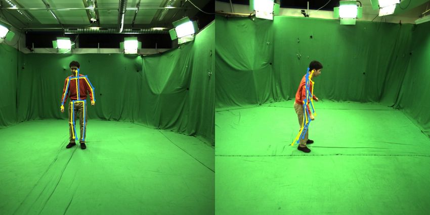

PhysCap: Physically Plausible Monocular 3D Motion Capture in Real Time • 235:5

 Input Image
 Stage I: Stage III:
 Kinematic Pose Estimation Physics-Based
 Global Pose Optimisation
 Output

 Stage I: Kinematic Pose Estimation Stage II: Foot Contact and Motion State Prediction
 CNN 2D Heatmaps 3D Location Maps Skeleton Fitting

 Stage III: Physics-Based Global Pose Optimisation
 Iterate Times

 i) Kinematic ii) Set iv) Pose Tracking
 v) Pose Update
 Pose Correction PD Controller Optimisation
 iii) GRF
 Estimation

Fig. 3. Overview of our pipeline. In stage I, the 3D pose estimation network accepts RGB image I as input and returns 2D joint keypoints K along with
the global 3D pose q 
 , i.e., root translation, orientation and joint angles of a kinematic skeleton. In stage II, K is fed to the contact and motion state
 
detection network. Stage II returns the contact states of heels and forefeet as well as a label b that represents if the subject in I is stationary or not. In stage
III, q 
 and b are used to iteratively update the character pose respecting physics laws. After the pose update iterations, we obtain the final 3D pose
q ℎ . Note that the orange arrows in stage III represent the steps that are repeated in the loop in every iteration. Kinematic pose correction is performed
 
only once at the beginning of stage III.

is estimated from a monocular image sequence (see stage I in Fig. 3), so far into stationary and non-stationary – this is stored in one
which contains physically implausible artefacts. Solving for joint binary flag. It also estimates binary foot-floor contact flags, i.e., for
torque controls that blindly make the character follow, would make the toes and heels of both feet, resulting in four binary flags (Sec. 4.2).
the character quickly fall down. Hence, we keep the first six entries This stage outputs the combined state vector b ∈ R5 .
of in our formulation and can thus directly control the root posi- The third and final stage of PhysCap is the physically plausible
tion and orientation with an additional external force. This enables global 3D pose estimation (Sec. 4.3). It combines the estimates from
the final character motion to keep up with the global root trajectory the first two stages with physics-based constraints to yield a physi-
estimated in the first stage of PhysCap, without falling down. cally plausible real-time 3D motion capture result that adheres to
 physics-based posture and environment constraints q ℎ ∈ R . In
 the following, we describe each of the stages in detail.
4 METHOD
Our PhysCap approach includes three stages, see Fig. 3 for an
overview. The first stage performs kinematic pose estimation. This 4.1 Stage I: Kinematic Pose Estimation
encompasses 2D heatmap and 3D location map regression for each Our kinematic pose estimation stage follows the real-time VNect
body joint with a CNN, followed by a model-based space-time pose algorithm [Mehta et al. 2017b], see Fig. 3, stage I. We first predict
optimisation step (Sec. 4.1). This stage returns 3D skeleton pose in heatmaps of 2D joints and root-relative location maps of joint po-
 
joint angles q ∈ R along with the 2D joint keypoints K ∈ R ×2 sitions in 3D with a specially tailored fully convolutional neural
for every image; denotes the number of 2D joint keypoints. As network using a ResNet [He et al. 2016] core. The ground truth joint
 
explained earlier, this initial kinematic reconstruction q is prone locations for training are taken from the MPII [Andriluka et al. 2014]
to physically implausible effects such as foot-floor penetration, foot and LSP [Johnson and Everingham 2011] datasets in the 2D case,
skating, anatomically implausible body leaning and temporal jitter, and MPI-INF-3DHP [Mehta et al. 2017a] and Human3.6m [Ionescu
especially notable along the depth dimension. et al. 2013] datasets in the 3D case.
 The second stage performs foot contact and motion state detection, Next, the estimated 2D and 3D joint locations are temporally
which uses 2D joint detections K to classify the poses reconstructed filtered and used as constraints in a kinematic skeleton fitting step

 ACM Trans. Graph., Vol. 39, No. 6, Article 235. Publication date: December 2020.

235:6 • Soshi Shimada, Vladislav Golyanik, Weipeng Xu, and Christian Theobalt

a) balanced posture b) unbalanced posture

 : Centre of Gravity
 (CoG)

 (a) (b) (c)

 Left foot Left foot Fig. 5. (a) An exemplary frame from the Human 3.6M dataset with the
 : Base of Support ground truth reprojections of the 3D joint keypoints. The magnified view
 : Projected CoG in the red rectangle shows the reprojected keypoint that deviates from the
 Right foot Right foot onto ground rotation centre (the middle of the knee). (b) Schematic visualisation of the
 reference motion correction. Readers are referred to Sec. 4.3.1 for its details.
 (c) Example of a visually unnatural standing (stationary) pose caused by
Fig. 4. (a) Balanced posture: the CoG of the body projects inside the base of physically implausible knee bending.
support. (b) Unbalanced posture: the CoG does not project inside the base
of support, which causes the human to start losing a balance.
 to know foot-floor contact states. Another important aspect of the
 physical plausibility of biped poses, in general, is balance. When
that optimises the following energy function: a human is standing or in a stationary upright state, the CoG of
 
 E (q 
 ) =EIK (q 
 ) + Eproj. (q )+ her body projects inside a base of support (BoS). The BoS is an
 (3) area on the ground bounded by the foot contact points, see Fig. 4
 
 Esmooth (q ) + Edepth (q ). for a visualisation. When the CoG projects outside the BoS in a
The energy function (3) contains four terms (see [Mehta et al. 2017b]), stationary pose, a human starts losing balance and will fall if no
i.e., the 3D inverse kinematics term EIK , the projection term Eproj. , correcting motion or step is applied. Therefore, maintaining a static
the temporal stability term Esmooth and the depth uncertainty cor- pose with an extensive leaning, as often observed in the results of
rection term Edepth . EIK is the data term which constrains the 3D monocular pose estimation, is not physically plausible (Fig .4-(b)).
pose to be close to the 3D joint predictions from the CNN. Eproj. The aforementioned CoG projection criterion can be used to correct
enforces the pose q to reproject it to the 2D keypoints (joints) imbalanced stationary poses [Coros et al. 2010; Faloutsos et al. 2001;
detected by the CNN. Note that this reprojection constraint, to- Macchietto et al. 2009]. To perform such correction in stage III, we
gether with calibrated camera and calibrated bone lengths, enables need to know if a pose is stationary or non-stationary (whether it
computation of the global 3D root (pelvis) position in the camera is a part of a locomotion/walking phase).
space. Temporal stability is further imposed by penalising the root’s Stage II, therefore, estimates foot-floor contact states of the feet
acceleration and variations along the depth channel by Esmooth and in each frame and determines whether the pose of the subject in I 
Edepth , respectively. The energy (3) is optimised by non-linear least is stationary or not. To predict both, i.e., foot contact and motion
squares (Levenberg-Marquardt algorithm [Levenberg 1944; Mar- states, we use a neural network whose architecture extends Zou et
quardt 1963]), and the obtained vector of joint angles and the root al. [2020] who only predict foot contacts. It is composed of temporal
 
rotation and position q of a skeleton with fixed bone lengths are convolutional layers with one fully connected layer at the end. The
smoothed by an adaptive first-order low-pass filter [Casiez et al. network takes as input all 2D keypoints K from the last seven
2012]. Skeleton bone lengths of a human can be computed, up to time steps (the temporal window size is set to seven), and returns
a global scale, from averaged 3D joint detections of a few initial for each image frame binary labels indicating whether the subject
frames. Knowing the metric height of the human determines the is in the stationary or non-stationary pose, as well as the contact
scale factor to compute metrically correct global 3D poses. state flags for the forefeet and heels of both feet encompassed in b .
 The result of stage I is a temporally-consistent joint angle se- The supervisory labels for training this network are automatically
quence but, as noted earlier, captured poses can exhibit artefacts computed on a subset of the 3D motion sequences of the Human3.6M
and contradict physical plausibility (e.g., evince floor penetration, [Ionescu et al. 2013] and DeepCap [Habermann et al. 2020] datasets
incorrect body leaning, temporal jitter, etc.). using the following criteria: the forefoot and heel joint contact labels
 are computed based on the assumption that a joint in contact is not
4.2 Stage II: Foot Contact and Motion State Detection sliding, i.e., the velocity is lower than 5 cm/sec. In addition, we use
 a height criterion, i.e., the forefoot/heel, when in contact with the
The ground reaction force (GRF) – applied when the feet touch
 floor, has to be at a 3D height that is lower than a threshold ℎ thres. . To
the ground – enables humans to walk and control their posture.
 determine this threshold for each sequence, we calculate the average
The interplay of internal body forces and the ground reaction force 
controls human pose, which enables locomotion and body balancing heel ℎℎ 
 avg and forefoot ℎ avg heights for each subject using the
by controlling the centre of gravity (CoG). To compute physically first ten frames (when both feet touch the ground). Thresholds are
 
plausible poses accounting for the GRF in stage III, we thus need then computed as ℎℎ thres.
 = ℎℎ 
 avg + 5cm for heels and ℎ thres. =

ACM Trans. Graph., Vol. 39, No. 6, Article 235. Publication date: December 2020.

PhysCap: Physically Plausible Monocular 3D Motion Capture in Real Time • 235:7

ℎ avg + 5cm for the forefeet. This second criterion is needed since, estimated 3D pose q is often not physically plausible. Therefore,
otherwise, a foot in the air that is kept static could also be labelled prior to torque-based optimisation, we pre-correct a pose q from
as being in contact. stage I if it is 1) stationary and 2) unbalanced, i.e., the CoG projects
 We also automatically label stationary and non-stationary poses outside the BoS. If both correction criteria are fulfilled, we compute
on the same sequences. When standing and walking, the CoG of the angle between the ground plane normal and the vector 
the human body typically lies close to the pelvis in 3D, which cor- that defines the direction of the spine relative to the root in the local
responds to the skeletal root position in both the Human3.6M and character’s coordinate system (see Fig. 5-(b) for the schematic visu-
DeepCap datasets. Therefore, when the velocity of 3D root is lower alisation). We then correct the orientation of the virtual character
than a threshold , we classify the pose as stationary, and non- towards a posture, for which CoG projects inside BoS. Correcting
stationary otherwise. In total, around 600 sets of contact and mo- in one large step could lead to instabilities in physics-based pose
tion state labels for the human images are generated. optimisation. Instead, we reduce by a small rotation of the virtual
 character around its horizontal axis (i.e., the axis passing through
4.3 Stage III: Physically Plausible Global 3D Pose the transverse plane of a human body) starting with the corrective
 Estimation angle = 10 for the first frame. Thereby, we accumulate the degree
 
Stage III uses the results of stages I and II as inputs, i.e., q and of correction in for the subsequent frames, i.e., +1 = + 10 .
 . It transforms the kinematic motion estimate into a physically Note that is decreasing for every frame and the correction step
plausible global 3D pose sequence that corresponds to the images is performed for all subsequent frames until 1) the pose becomes
and adheres to anatomy and environmental constraints imposed non-stationary or 2) CoG projects inside BoS1 .
by the laws of physics. To this end, we represent the human as However, simply correcting the spine orientation by the skeleton
a torque-controlled simulated character with a floating base and rotation around the horizontal axis can lead to implausible standing
PD joint controllers [A. Salem and Aly 2015]. The core is to solve poses, since the knees can still be unnaturally bent for the obtained
an energy-based optimisation problem to find the vector of forces upright posture (see Fig. 5-(c) for an example). To account for that,
 and accelerations q¥ of the character such that the equations of we adjust the respective DoFs of the knees and hips such that the
motion with constraints are fulfilled (Sec. 4.3.5). This optimisation relative orientation between upper legs and spine, as well as upper
is preceded by several preprocessing steps applied to each frame. and lower legs, are more straight. The hip and knee correction
 
 First i), we correct q if it is strongly implausible based on starts if both correction criteria are still fulfilled and is already
several easy-to-test criteria (Sec. 4.3.1). Second ii), we estimate the very small. Similarly to the correction, we introduce accumulator
desired acceleration q¥ ∈ R necessary to reproduce q based variables for every knee and every hip. The correction step for
on the PD control rule (Secs. 4.3.2). Third iii), in input frames in knees and hips is likewise performed until 1) the pose becomes
which a foot is in contact with the floor (Sec. 4.3.3), we estimate the non-stationary or 2) CoG projects inside BoS1 .
ground reaction force (GRF) (Sec. 4.3.4). Fourth iv), we solve the
optimisation problem (10) to estimate and accelerations q¥ where 4.3.2 Computing the Desired Accelerations. To control the physics-
the equation of motion with the estimated GRF and the contact based virtual character such that it reproduces the kinematic esti-
 , we set the desired joint acceleration q
 mate q ¥ following the
constraint to avoid foot-floor penetration (Sec. 4.3.5) are integrated
as constraints. Note that the contact constraint is integrated only PD controller rule:
when the foot is in contact with the floor. Otherwise, only the 
 q¥ = q¥ + (q − q) + ( q¤ − q¤ ). (4)
equation of motion without GRF is introduced as a constraint in
(10). v) Lastly, the pose is updated using the finite-difference method The desired acceleration q¥ is later used in the GRF estimation
(Eq. (1)) with the estimated acceleration q¥ . The steps ii) - v) are step (Sec. 4.3.4) and the final pose optimisation (Sec. 4.3.5). Con-
iterated = 4 times for each frame of video. trolling the character motion on the basis of a PD controller in the
 As also observed by [Andrews et al. 2016], this two-step optimi- system enables the character to exert torques which reproduce the
sation iii) and iv) reduces direct actuation of the character’s root kinematic estimate q while significantly mitigating undesired
as much as possible (which could otherwise lead to slightly un- effects such as joint and base position jitter.
natural locomotion), and explains the kinematically estimated root
position and orientation by torques applied to other joints as much 4.3.3 Foot-Floor Collision Detection. To avoid foot-floor penetra-
as possible when there is a foot-floor contact. Moreover, this two- tion in the final pose sequence and to mitigate contact position
step optimisation is computationally less expensive rather than sliding, we integrate hard constraints in the physics-based pose
estimating q¥ , and simultaneously [Zheng and Yamane 2013]. optimisation to enforce zero velocity of forefoot and heel links in
Our algorithm thus finds a plausible balance between pose accuracy, Sec. 4.3.5. However, these constraints can lead to unnatural motion
physical accuracy, the naturalness of captured motion and real-time in rare cases when the state prediction network may fail to estimate
performance. the correct foot contact states (e.g., when the foot suddenly stops
 in the air while walking). We thus update the contact state output
4.3.1 Pose Correction. Due to the error accumulation in stage I ′
 of the state prediction network b , ∈ {1,...,4} , to yield b , as
(e.g., as a result of the deviation of 3D annotations from the joint ∈ {1,...,4}

rotation centres in the skeleton model, see Fig. 5-(a), as well as inac-
curacies in the neural network predictions and skeleton fitting), the 1 either after the correction or already in q 
 provided by stage I

 ACM Trans. Graph., Vol. 39, No. 6, Article 235. Publication date: December 2020.

235:8 • Soshi Shimada, Vladislav Golyanik, Weipeng Xu, and Christian Theobalt

follows: Table 1. Names and duration of our six newly recorded outdoor sequences
 captured using SONY DSC-RX0 at 25 fps.
 
 
  1, b 
 if ( = 1 and ℎ < ) or
 ′
 
 
 b , ∈{1,...,4} = the -th link collides with the floor plane, (5)
  Sequence ID Sequence Name Duration [sec]
  0,
 
 otherwise.
  1 building 1 132
This means we consider a forefoot or heel link to be in contact only 2 building 2 90
if its height ℎ is less than a threshold = 0.1m above the calibrated 3 forest 105
ground plane. 4 backyard 60
 In addition, we employ the Pybullet [Coumans and Bai 2016] 5 balance beam 1 21
physics engine to detect foot-floor collision for the left and right 6 balance beam 2 12
foot links. Note that combining the mesh collision information
with the predictions from the state prediction network is necessary
 (Sec. 4.3.4) in the equation of motion. In addition, we introduce
because 1) the foot may not touch the floor plane in the simulation
 contact constraints to prevent foot-floor penetration and foot slid-
when the subject’s foot is actually in contact with the floor due to
 , and 2) the foot can penetrate into the mesh ing when contacts are detected.
the inaccuracy of q 
 Let r¤ be the velocity of the -th contact link. Then, using the
floor plane if the network misdetects the contact state when there
 relationship between r¤ and q¤ [Featherstone 2014], we can write:
is actually a foot contact in I .
 J q¤ = r¤ . (8)
4.3.4 Ground Reaction Force (GRF) Estimation. We first compute
the GRF – when there is a contact between a foot and floor – When the link is in contact with the floor, the velocity perpendicular
which best explains the motion of the root as coming from stage to the floor has to be zero or positive to prevent penetration. Also,
I. However, the target trajectory from stage I can be physically we allow the contact links to have a small tangential velocity 
implausible, and we will thus eventually also require a residual force to prevent an immediate foot motion stop which creates visually
directly applied on the root to explain the target trajectory; this unnatural motion. Our contact constraint inequalities read:
force will be computed in the final optimisation. To compute the 0 ≤ ¤ , | ¤ | ≤ , and | ¤ | ≤ , (9)
GRF, we solve the following minimisation problem:
 where ¤ is the normal component of r¤ , and ¤ along with ¤ are
 min ∥M1 q¥ − J 1 G ∥, the tangential elements of r¤ .
 (6)
 s.t. ∈ , Using the desired acceleration q¥ (Eq. (4)), the equation of mo-
 tion (2), optimal GRF estimated in (6) and contact constraints (9),
where ∥·∥ denotes ℓ 2 -norm, and M1 ∈ R 6× together with J 1 ∈
 we formulate the optimisation problem for finding the physics-based
R 6×6 are the first six rows of M and J that correspond to the motion capture result as:
root joint, respectively. Since we do not consider sliding contact,
the contact force has to satisfy friction cone constraints. Thus, we min ∥ q¥ − q¥ ∥ + ∥ ∥,
 q¥ , 
formulate a linearised friction cone constraint . That is, s.t. M¥q − = J G − c(q, q¤ ), and (10)
 n o
 = ∈ R 3 | > 0, ≤ 
 
 ¯ , ≤ 
 
 ¯ , (7) 0 ≤ ¤ , | ¤ | ≤ , | ¤ | ≤ , ∀ .
 The first energy term forces the character to reproduce q . The
 
where is a normal component, and are the tangential second energy term is the regulariser that minimises to prevent
components of a contact force at the -th contact position; is the overshooting, thus modelling natural human-like motion.
a friction coefficient which we set to 0.8 and the √friction coefficient After solving (10), the character pose is updated by Eq. (1). We
of inner linear cone approximation reads ¯ = / 2. iterate the steps ii) - v) (see stage III in Fig. 3) = 4 times, and stage
 The GRF is then integrated into the subsequent optimisation III returns the -th output from v) as the final character pose q ℎ .
step (10) to estimate torques and accelerations of all joints in the
 The final output of stage III is a sequence of joint angles and global
body, including an additional residual direct root actuation compo-
 root translations and rotations that explains the image observations,
nent that is needed to explain the difference between the global 3D
 follows the purely kinematic reconstruction from stage I, yet is
root trajectory of the kinematic estimate and the final physically
 physically and anatomically plausible and temporally stable.
correct result. The aim is to keep this direct root actuation as small
as possible, which is best achieved by a two-stage strategy that first 5 RESULTS
estimates the GRF separately. Moreover, we observed this two-step
 We first provide implementation details of PhysCap (Sec. 5.1) and
optimisation enables faster computation than estimating , q¥ and 
 then demonstrate its qualitative state-of-the-art results (Sec. 5.2).
all at once. It is hence more suitable for our approach which aims at
 We next evaluate PhysCap’s performance quantitatively (Sec. 5.3)
real-time operation.
 and conduct a user study to assess the visual physical plausibility
4.3.5 Physics-Based Pose Optimisation. In this step, we solve an of the results (Sec. 5.4).
 
optimisation problem to estimate and q¥ to track q using the We test PhysCap on widely-used benchmarks [Habermann et al.
equation of motion (2) as a constraint. When contact is detected 2020; Ionescu et al. 2013; Mehta et al. 2017a] as well as on backflip
(Sec. 4.3.3), we integrate the estimated ground reaction force and jump sequences provided by [Peng et al. 2018]. We also collect

ACM Trans. Graph., Vol. 39, No. 6, Article 235. Publication date: December 2020.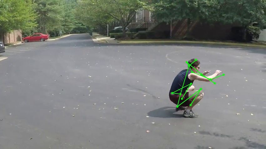

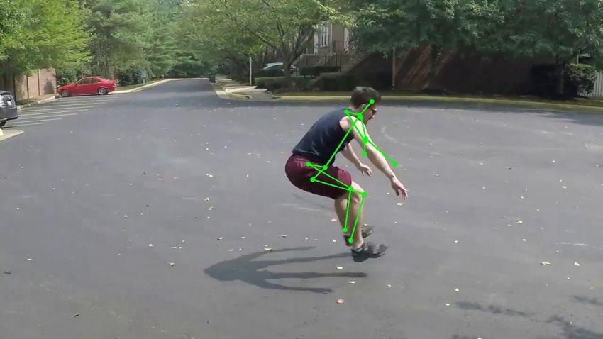
PhysCap: Physically Plausible Monocular 3D Motion Capture in Real Time • 235:9

a) Frontal View Reference View Frontal View Reference View
 Time

2D Projection

 3D Pose

b)

2D Projection

 Fig. 7. Reprojected 3D keypoints onto two different images with different
 view angles for squatting. Frontal view images are used as inputs and images
 3D Pose of the reference view are used only for quantitative evaluation. Our results
 are drawn in light blue, wheres the results by VNect [Mehta et al. 2017b] are
 provided in yellow. Our reprojections are more feasible, which is especially
 noticeable in the reference view. See also our supplementary video.

Fig. 6. Two examples of reprojected 3D keypoints obtained by our ap-
proach (light blue colour) and Vnect [Mehta et al. 2017b] (yellow colour) employ the Pybullet [Coumans and Bai 2016] as a physics engine
together with the corresponding 3D visualisations from different view angles. for the character motion visualisation and collision detection. In
PhysCap produces much more natural and physically plausible postures this paper, we set the proportional gain value and derivative
whereas Vnect suffers from unnatural body leaning (see also the supple- gain value for all joints to 300 and 20, respectively. For the root
mentary video).
 angular acceleration, and are set to 340 and 30, respectively.
 and of the root linear acceleration are set to 1000 and 80,
a new dataset with various challenging motions. It features six respectively. These settings are used in all experiments.
sequences in general scenes performed by two subjects2 recorded
at 25 fps. For the recording, we used SONY DSC-RX0, see Table 1 5.2 Qualitative Evaluation
for more details on the sequences. The supplementary video and result figures in this paper, in particu-
 lar Figs. 1 and 11 show that PhysCap captures global 3D human poses
5.1 Implementation in real time, even of fast and difficult motions, such as a backflip
Our method runs in real time (25 fps on average) on a PC with and a jump, which are of significantly improved quality compared
a Ryzen7 2700 8-Core Processor, 32 GB RAM and GeForce RTX to previous monocular methods. In particular, captured motions
2070 graphics card. In stage I, we proceed from a freely available are much more temporally stable, and adhere to laws of physics
demo version of VNect [Mehta et al. 2017b]. Stages II and III are with respect to the naturalness of body postures and fulfilment of
implemented in python. In stage II, the network is implemented environmental constraints, see Figs. 6–8 and 10 for the examples of
with PyTorch [Paszke et al. 2019]. In stage III, we use the Rigid Body more natural 3D reconstructions. These properties are essential for
Dynamics Library [Felis 2017] to compute dynamic quantities. We many applications in graphics, in particular for stable real-time char-
2 thevariety of motions per subject is high; there are only two subjects in the new acter animation, which is feasible by directly applying our method’s
dataset due to COVID-19 related recording restrictions output (see Fig. 1 and the supplementary video).

 ACM Trans. Graph., Vol. 39, No. 6, Article 235. Publication date: December 2020.

235:10 • Soshi Shimada, Vladislav Golyanik, Weipeng Xu, and Christian Theobalt

 of testing a method on multiple sequences and reporting the accu-
 racy of 3D joint positions as well as the accuracy of the reprojection
 into the input views. The accuracy in 3D is evaluated by mean per
 joint position error (MPJPE) in mm, percentage of correct keypoints
 (PCK) and the area under the receiver operating characteristic (ROC)
 curve abbreviated as AUC. The reprojection or mean pixel error
 input
 2 is obtained by projecting the estimated 3D joints onto the in-
 put images and taking the average per frame distance to the ground
 input
 truth 2D joint positions. We report 2 and its standard deviation
 input
 denoted by 2 with the images of size 1024 × 1024 pixels.
 As explained earlier, these metrics only evaluate limited aspects
 of captured 3D poses and do not account for essential aspects of
 temporal stability, smoothness and physical plausibility in recon-
 structions such as jitter, foot sliding, foot-floor penetration and
 unnaturally balanced postures. As we show in the supplemental
 video, top-performing methods on MPJPE and 3D PCK can fare
 poorly with respect to these criteria. Moreover, MPJPE and PCK
 are often reported after rescaling of the result in 3D or Procrustes
 alignment, which further makes these metrics agnostic to the afore-
 mentioned artefacts. Thus, we introduce four additional metrics
 which allow to evaluate the physical plausibility of the results, i.e.,
 reprojection error to unseen views 2 side , motion jitter error 
 ℎ
 and two floor penetration errors – Mean Penetration Error (MPE)
 and Percentage of Non-Penetration (PNP).
 When choosing a reference side view for 2 side , we make sure
 that the viewing angle between the input and side views has to be
 sufficiently large, i.e., more than ∼ 15 . Otherwise, if a side view is
 close to the input view, such effects as unnatural leaning forward
Fig. 8. Several visualisations of the results by our approach and VNect can still remain undetected by 2 side in some cases. After reprojection
[Mehta et al. 2017b]. The first and second rows show our estimated 3D of a 3D structure to an image plane of a side view, all further steps for
poses after reprojection in the input image and its 3D view, respectively. side are similar to the steps for the standard reprojection
 calculating 2 
Similarly, the third and fourth rows show the reprojected 3D pose and 3D side , i.e., the standard deviation of side .
view for VNect. Note that our motion capture shows no foot penetration error. We also report 2 2 
into the floor plane whereas such artefact is apparent in the VNect results. To quantitatively compare the motion jitter, we report the devi-
 ation of the temporal consistency from the ground truth 3D pose.
 Our smoothness error ℎ is computed as follows:
5.3 Quantitative Evaluation , −1
 =∥p , 
 − p ∥,
In the following, we first describe our evaluation methodology in , , −1
Sec. 5.3.1. We evaluate PhysCap and competing methods under a va- =∥p − p ∥, (11)
 ℎ = 1 Í Í | − |,
riety of criteria, i.e., 3D joint position, reprojected 2D joint positions, =1 =1 
foot penetration into the floor plane and motion jitter. We compare
our approach with current state-of-the-art monocular pose estima- where p , represents the 3D position of joint in the time frame . 
tion methods,i.e., HMR [Kanazawa et al. 2018], HMMR [Kanazawa and denote the total numbers of frames in the video sequence and
et al. 2019] and Vnect [Mehta et al. 2017b] (here we use the so-called target 3D joints, respectively. The subscripts and stand for the
demo version provided by the authors with further improved ac- predicted output and ground truth, respectively. A lower ℎ
curacy over the original paper due to improved training). For the indicates lower motion jitter in the predicted motion sequence.
comparison, we use the benchmark dataset Human3.6M [Ionescu MPE and PNP measure the degree of non-physical foot penetra-
et al. 2013], the DeepCap dataset [Habermann et al. 2020] and MPI- tion into the ground. MPE is the mean distance between the floor
INF-3DHP [Mehta et al. 2017a]. From the Human3.6M dataset, we and 3D foot position, and it is computed only when the foot is in
use the subset of actions that does not have occluding objects in the contact with the floor. We use the ground truth foot contact labels
frame, i.e., directions, discussions, eating, greeting, posing, purchases, (Sec. 4.2) to judge the presence of the actual foot contacts. The com-
taking photos, waiting, walking, walking dog and walking together. plementary PNP metric shows the ratio of frames where the feet
From the DeepCap dataset, we use the subject 2 for this comparison. are not below the floor plane over the entire sequence.

5.3.1 Evaluation Methodology. The established evaluation method- 5.3.2 Quantitative Evaluation Results. Table 2 summarises MPJPE,
ology in monocular 3D human pose estimation and capture consists PCK and AUC for root-relative joint positions with (first row) and

ACM Trans. Graph., Vol. 39, No. 6, Article 235. Publication date: December 2020.

PhysCap: Physically Plausible Monocular 3D Motion Capture in Real Time • 235:11

Table 2. 3D error comparison on benchmark datasets with VNect [Mehta et al. 2017b], HMR [Kanazawa et al. 2018] and HMMR [Kanazawa et al. 2019]. We
report the MPJPE in mm, PCK at 150 mm and AUC. Higher AUC and PCK are better, and lower MPJPE is better. Note that the global root positions for HMR
and HMMR were estimated by solving optimisation with a 2D projection loss using the 2D and 3D keypoints obtained from the methods. Our method is on
par with and often close to the best-performing approaches on all datasets. It consistently produces the best global root trajectory. As indicated in the text,
these widely-used metrics in the pose estimation literature only paint an incomplete picture. For more details, please refer Sec. 5.3.

 DeepCap Human 3.6M MPI-INF-3DHP
 MPJPE [mm] ↓ PCK[%] ↑ AUC[%]↑ MPJPE [mm] ↓ PCK[%] ↑ AUC[%]↑ MPJPE [mm] ↓ PCK[%] ↑ AUC[%]↑
 ours 68.9 95.0 57.9 65.1 94.8 60.6 104.4 83.9 43.1
 Vnect 68.4 94.9 58.3 62.7 95.7 61.9 104.5 84.1 43.2
 Procrustes
 HMR 77.1 93.8 52.4 54.3 96.9 66.6 87.8 87.1 50.9
 HMMR 75.5 93.8 53.1 55.0 96.6 66.2 106.9 79.5 44.8
 ours 113.0 75.4 39.3 97.4 82.3 46.4 122.9 72.1 35.0
 Vnect 102.4 80.2 42.4 89.6 85.1 49.0 120.2 74.0 36.1
 no Procrustes
 HMR 113.4 75.1 39.0 78.9 88.2 54.1 130.5 69.7 35.7
 HMMR 101.4 81.0 42.0 79.4 88.4 53.8 174.8 60.4 30.8
 ours 110.5 80.4 37.0 182.6 54.7 26.8 257.0 29.7 15.3
 Vnect 112.6 80.0 36.8 185.1 54.1 26.5 261.0 28.8 15.0
 global root position
 HMR 251.4 19.5 8.4 204.2 45.8 22.1 505.0 28.6 13.5
 HMMR 213.0 27.7 11.3 231.1 41.6 19.4 926.2 28.0 14.5

Table 3. 2D projection error of a frontal view (input) and side view (non- Table 4. Comparison of temporal smoothness on the DeepCap [Haber-
input) on DeepCap dataset [Habermann et al. 2020]. PhysCap performs mann et al. 2020] and Human 3.6M datasets [Ionescu et al. 2013]. PhysCap
similarly to VNect on the frontal view, and significantly better on the side significantly outperforms VNect and HMR, and fares comparably to HMMR
view. For further details, see Sec. 5.3 and Fig. 7 in terms of this metric. For a detailed explanation, see Sec. 5.3.

 Front View Side View Ours Vnect HMR HMMR
 input input side [pixel] side
 2 [pixel] 2 2 2 ℎ 6.3 11.6 11.7 8.1
 DeepCap
 Ours 21.1 6.7 35.5 16.8 ℎ 4.1 8.6 9.0 5.1
 Vnect [Mehta et al. 2017b] 14.3 2.7 37.2 18.1 ℎ 7.2 11.2 11.2 6.8
 Human 3.6M
 ℎ 6.9 10.1 12.7 5.9
without (second row) Procrustes alignment before the error compu-
tation for our and related methods. We also report the global root
 Table 5. Comparison of Mean Penetration Error (MPE) and Percentage
position accuracy in the third row. Since HMR and HMMR do not
 of Non-Penetration (PNP) on DeepCap dataset [Habermann et al. 2020].
return global root positions as their outputs, we estimate the root PhysCap significantly outperforms VNect on this metric, measuring an
translation in 3D by solving an optimisation with 2D projection essential aspect of physical motion correctness.
energy term using the 2D and 3D keypoints obtained from these
algorithms (similar to the solution in VNect). The 3D bone lengths MPE [mm] ↓ ↓ PNP [%] ↑
of HMR and HMMR were rescaled so that they match the ground Ours 28.0 25.9 92.9
truth bone lengths. Vnect [Mehta et al. 2017b] 39.3 37.5 45.6
 In terms of MPJPE, PCK and AUC, our method does not outper-
form the other approaches consistently but achieves an accuracy
that is comparable and often close to the highest on Human3.6M,
DeepCap and MPI-INF-3DHP. In the third row, we additionally explicitly models physical pose plausibility, it excels VNect in the
evaluate the global 3D base position accuracy, which is critical for side view, which reveals VNect’s implausibly leaning postures and
character animation from the captured data. Here, PhysCap consis- root position instability in depth, also see Figs. 6 and 7.
tently outperforms the other methods on all the datasets. To assess motion smoothness, we report ℎ and its standard
 As noted earlier, the above metrics only paint an incomplete deviation ℎ in Table 4. Our approach outperforms Vnect and
picture. Therefore, we also measure the 2D projection errors to the HMR by a big margin on both datasets. Our method is better than
input and side views on the DeepCap dataset, since this dataset HMMR on DeepCap dataset and marginally worse on Human3.6M.
includes multiple synchronised views of dynamic scenes with a HMMR is one of the current state-of-the-art algorithms that has an
 input explicit temporal component in the architecture.
wide baseline. Table 3 summarises the mean pixel errors 2 and
 side together with their standard deviations. In the frontal view, i.e.,
 Table 5 summarises the MPE and PNP for Vnect and PhysCap
 2 on DeepCap dataset. Our method shows significantly better results
 input
on 2 , VNect has higher accuracy than PhysCap. However, this compared to VNect, i.e., about a 30% lower MPE and a by 100%
comes at the prize of frequently violating physics constraints (floor better result in PNP, see Fig. 8 for qualitative examples. Fig. 9 shows
penetration) and producing unnaturally leaning and jittering 3D plots of contact forces as the functions of time calculated by our
poses (see also the supplemental video). In contrast, since PhysCap approach on the walking sequence from our newly recorded dataset

 ACM Trans. Graph., Vol. 39, No. 6, Article 235. Publication date: December 2020.