ALMA resolves giant molecular clouds in a tidal dwarf galaxy

A&A 645, A97 (2021)
https://doi.org/10.1051/0004-6361/202038955 Astronomy
c ESO 2021 &
 Astrophysics

 ALMA resolves giant molecular clouds in a tidal dwarf galaxy? , ??
M. Querejeta1 , F. Lelli2 , E. Schinnerer3 , D. Colombo4 , U. Lisenfeld5,6 , C. G. Mundell7 , F. Bigiel8 , S. García-Burillo1 ,
 C. N. Herrera9 , A. Hughes10,11 , J. M. D. Kruijssen12 , S. E. Meidt13 , T. J. T. Moore14 , J. Pety9,15 , and A. J. Rigby2

 1
 Observatorio Astronómico Nacional, Alfonso XII, 3, 28014 Madrid, Spain
 e-mail: m.querejeta@oan.es
 2
 School of Physics and Astronomy, Cardiff University, 5 The Parade, CF24 3AA Cardiff, UK
 3
 Max-Planck-Institut für Astronomie, Königstuhl 17, 69117 Heidelberg, Germany
 4
 Max-Planck-Institut für Radioastronomie, Auf dem Hügel 9, 53121 Bonn, Germany
 5
 Departamento de Física Teórica y del Cosmos, Universidad de Granada, 18071 Granada, Spain
 6
 Instituto Carlos I de Física Teórica y Computacional, Facultad de Ciencias, 18071 Granada, Spain
 7
 Department of Physics, University of Bath, Claverton Down, Bath BA2 7AY, UK
 8
 Argelander-Institut für Astronomie, Universität Bonn, Auf dem Hügel 71, 53121 Bonn, Germany
 9
 IRAM, 300 rue de la Piscine, 38406 Saint Martin, d’Hères, France
 10
 Université de Toulouse, UPS-OMP, 31028 Toulouse, France
 11
 CNRS, IRAP, Av. du Colonel Roche BP 44346, 31028 Toulouse Cedex 4, France
 12
 Astronomisches Rechen-Institut, Zentrum für Astronomie der Universität Heidelberg, Mönchhofstraße 12-14, 69120 Heidelberg,
 Germany
 13
 Sterrenkundig Observatorium, Universiteit Gent, Krijgslaan 281 S9, 9000 Gent, Belgium
 14
 Astrophysics Research Institute, Liverpool John Moores University, IC2, Liverpool Science Park, 146 Brownlow Hill, Liverpool
 L3 5RF, UK
 15
 Sorbonne Université, Observatoire de Paris, Université PSL, CNRS, LERMA, 75005 Paris, France

 Received 16 July 2020 / Accepted 30 October 2020

 ABSTRACT

 Tidal dwarf galaxies (TDGs) are gravitationally bound condensations of gas and stars that formed during galaxy interactions. Here we
 present multi-configuration ALMA observations of J1023+1952, a TDG in the interacting system Arp 94, where we resolved CO(2–1)
 emission down to giant molecular clouds (GMCs) at 0.6400 ∼ 45 pc resolution. We find a remarkably high fraction of extended molecu-
 lar emission (∼80−90%), which is filtered out by the interferometer and likely traces diffuse gas. We detect 111 GMCs that give a sim-
 ilar mass spectrum as those in the Milky Way and other nearby galaxies (a truncated power law with a slope of −1.76 ± 0.13). We also
 study Larson’s laws over the available dynamic range of GMC properties (∼2 dex in mass and ∼1 dex in size): GMCs follow the size-
 mass relation of the Milky Way, but their velocity dispersion is higher such that the size-linewidth and virial relations appear super-
 linear, deviating from the canonical values. The global molecular-to-atomic gas ratio is very high (∼1) while the CO(2–1)/CO(1–0)
 ratio is quite low (∼0.5), and both quantities vary from north to south. Star formation predominantly takes place in the south of the
 TDG, where we observe projected offsets between GMCs and young stellar clusters ranging from ∼50 pc to ∼200 pc; the largest
 offsets correspond to the oldest knots, as seen in other galaxies. In the quiescent north, we find more molecular clouds and a higher
 molecular-to-atomic gas ratio (∼1.5); atomic and diffuse molecular gas also have a higher velocity dispersion there. Overall, the or-
 ganisation of the molecular interstellar medium in this TDG is quite different from other types of galaxies on large scales, but the
 properties of GMCs seem fairly similar, pointing to near universality of the star-formation process on small scales.
 Key words. galaxies: dwarf – galaxies: interactions – galaxies: star formation – galaxies: ISM – galaxies: kinematics and dynamics

1. Introduction lar populations, but this is not always the case (Fensch et al.
 2016). Such a dark matter-free setting, which is subject to tidal
When galaxies collide, a portion of the gas is ejected by tidal forces from their neighbours, affords the possibility of testing
forces and may eventually collapse under self-gravity, giving theories of star formation in an extreme dynamical environment.
rise to new low-mass galaxies along the tidal debris. These new- While TDGs have been extensively mapped through deep opti-
born systems, known as tidal dwarf galaxies (TDGs), are thought cal imaging, only a few studies have looked at their molecular
to be devoid of dark matter, but they retain the metallicity of gas content and distribution, and these studies target spatial res-
the galaxy from which they were originally stripped (Duc et al. olutions that are too coarse to resolve individual giant molecular
2000; Duc 2012; Lelli et al. 2015). TDGs tend to have high gas clouds (GMCs; e.g. Braine et al. 2000, 2001; Duc et al. 2007;
fractions and they are often active star-formers (Braine et al. Lisenfeld et al. 2016).
2001; Lisenfeld et al. 2016); many of them also host old stel- One of the most fundamental challenges of modern astro-
 ?
 Full Table A.3 is only available at the CDS via anonymous ftp physics is understanding the process by which gas transforms
to cdsarc.u-strasbg.fr (130.79.128.5) or via http://cdsarc. into stars, and how this process is orchestrated as a function
u-strasbg.fr/viz-bin/cat/J/A+A/645/A97 of the environment. Indeed, theories of galactic-scale star for-
 ??
 Movie is available at https://www.aanda.org mation and cosmological simulations of galaxy formation are

 Article published by EDP Sciences A97, page 1 of 20

A&A 645, A97 (2021)

both guided by the Kennicutt-Schmidt relation (Schmidt 1959; (traced by optical blue colours, Hα, and UV emission, as well as
Kennicutt 1998), the observed correlation between the star for- young stellar clusters resolved with HST; see Fig. 1).
mation rate surface density ΣSFR and neutral gas surface density There might be some evidence for low-level star formation in
Σgas (e.g. Schaye & Dalla Vecchia 2008; Semenov et al. 2018). the north-west of the TDG (see Sect. 4.4), but this is very limited
The correlation between star formation rates and the amount of compared to the vigorous star formation activity in the south.
molecular gas is also known to be very tight (e.g. Bigiel et al. Thus, we distinguish two environments within the TDG: the
2008; Schruba et al. 2011; Leroy et al. 2013). quiescent north and the star-forming south, separated by a dec-
 An increasing body of observational work suggests that, lination cut at Dec = 19◦ 510 5000 (Fig. 1). This cut is motivated
when molecular gas is probed down to GMC scales, its proper- by the two main concentrations of H i, which are connected by
ties depend on local physical conditions (Hughes et al. 2013b; a thin bridge on the eastern end. It might also be possible that
Colombo et al. 2014; Pan & Kuno 2017). Dynamical effects these two gas condensations correspond to two close-by but dis-
have been proposed to explain the differences in the state of tinct TDGs, but the existing H i data does not allow us to test
molecular gas and its ability to form stars (e.g. Luna et al. this scenario by studying their internal dynamics. The absence
2006; Meidt et al. 2018, 2013; Kruijssen et al. 2014; Renaud of detectable near-infrared continuum suggests a scarcity of old
et al. 2015). Cloud-cloud collisions have also been suggested stars in the TDG (M?old < 4.7×108 M corrected for our distance;
as a trigger of star formation (e.g. Tan 2000; Fujimoto et al. Mundell et al. 2004), implying that this must be a young TDG
2014; Dobbs et al. 2015; Torii et al. 2015). Several other fac- which might not be in dynamical equilibrium.
tors, such as changes in the incident radiation field, might fur- TDGs constitute exciting laboratories to study how gas
ther contribute to the observed differences in the shapes of assembles within a newborn galaxy. In particular, it is yet not
GMC mass spectra between M51, M33, and the Large Mag- known how quickly gas condenses into compact structures in
ellanic Cloud (Hughes et al. 2013a), or NGC 6946, NGC 628, such a pristine system and whether those structures are simi-
and M101 (Rebolledo et al. 2015). These environmental factors lar to the GMCs observed in our Galaxy or in external galax-
influence the ability of a GMC to form stars and, indirectly, the ies. To answer these questions, we present ALMA observations
shape of the Kennicutt-Schmidt relation, but their relative impor- of J1023+1952 which resolve the molecular emission down to
tance remains unknown. To understand the physics of star forma- GMC scales.
tion, it is crucial to probe conditions down to GMC scales, the In Sect. 2 we describe the ALMA data (Sect. 2.1) and a rich
units that are associated with massive star formation in our own set of ancillary data (Sect. 2.2). In Sect. 3, we identify and char-
Galaxy. acterise the GMCs. In Sect. 4 we present our results regarding
 J1023+1952 is a kinematically detached H i cloud in front the overall molecular structure (Sect. 4.1), the molecular gas
of the spiral galaxy NGC 3227, in the interacting system Arp 94 kinematics (Sect. 4.2), and the GMC properties and scaling rela-
 tions (Sect. 4.3). We discuss our results in Sect. 5 with a special
(Mundell et al. 1995b). Figure 1 shows our target in context,
 focus on the connection between GMC properties, local environ-
highlighting the large size of the Arp 94 system and its com-
 ment, and star formation. We close the paper with a summary in
plexity in terms of tidal tails as revealed by H i and deep optical
 Sect. 6.
emission. Specifically, the Arp 94 system is composed of a spi-
 We assume a distance of 14.5 ± 0.6 Mpc (Yoshii et al. 2014),
ral galaxy hosting a Seyfert 2 nucleus (NGC 3227; Mundell et al.
 based on a new AGN time lag method.
1995a; Schinnerer et al. 2001; Noda et al. 2014) interacting with
 As a consistency check, Yoshii et al. (2014) derived an inde-
a ‘green valley’ elliptical (NGC 3226; Appleton et al. 2014). The
 pendent value of H0 = (73 ± 3) km s−1 Mpc−1 from these dis-
TDG lies at the base of the northern tidal tail and partially over-
 tances, in agreement with the literature (e.g. Schombert et al.
laps in projection with the disc of NGC 3227. Since the TDG
 2020). For d = 14.5 Mpc, 100 corresponds to 70.3 pc. This is very
is obscuring stellar light from NGC 3227, it must be in front of
 similar to the d = 15.1 Mpc assumed by Mundell et al. (1995b)
the spiral galaxy (Mundell et al. 1995b, 2004). The total content
 based on the redshift of the source, and slightly smaller than
of atomic gas estimated by Mundell et al. (2004) in the TDG
 d = 20.4 Mpc assumed by Mundell et al. (2004) and Lisenfeld
is MHI = 1.9 × 108 M (corrected for our assumed distance),
 et al. (2008) relying on the Tully-Fisher relation (Tully 1988).
distributed over a projected area of 7 kpc × 5 kpc. As shown in
Fig. 1, active star formation is ongoing in the southern half of the
cloud, with blue knots clearly visible in Hα emission at veloc- 2. Data
ities that closely match those of the H i cloud, ruling out the
 2.1. ALMA data: Molecular gas emission
possibility that the star forming knots belong to the background
galaxy, which is offset in velocity by almost 300 km s−1 (Mundell We observed the CO(2–1) line with the ALMA Band 6
et al. 2004). Furthermore, the metallicity of these star-forming receiver (230 GHz) during Cycle 4 (project 2016.1.00648.S, PI:
knots is near-solar (12 + log(O/H) = 8.6; Lisenfeld et al. 2008), M. Querejeta). To recover emission from different spatial scales,
comparable to the metallicity of the spiral galaxy NGC 3227, and we combined the 12 m array with the Atacama Compact Array
much higher than the metallicity that would be expected for a (ACA, i.e. 7 m array and total power antennas). The 12 m array
dwarf galaxy of this luminosity (12+log(O/H) ' 8, according to observations were performed between 25 and 28 November
the magnitude-metallicity relation for classical dwarfs; Richer & 2016, with 46 antennas in C40-4 configuration, resulting in pro-
McCall 1995; Zhao et al. 2010). This strongly supports the idea jected baselines between 15 and 704 m which correspond to a
that J1023+1952 is a TDG and not a pre-existing dwarf captured typical angular resolution of 0.4−0.500 and a largest recoverable
by the Arp 94 system. angular scale of ≈400 . The 7 m observations were carried out
 Using the IRAM 30 m telescope, Lisenfeld et al. (2008) between 4 and 26 October 2016 (with 8–10 antennas), and the
demonstrated that this TDG is also rich in molecular gas (MH2 = total power, between 3 and 15 October 2016 (with 3–4 anten-
1.5 × 108 M , corrected for our distance). In spite of compara- nas). The 7 m-array data at the CO(2–1) frequency provides a
ble atomic and molecular gas surface densities in the north and resolution of ≈5.400 and a largest recoverable angular scale of
south of the cloud, star formation in J1023+1952 is predomi- ≈2900 , while ALMA total power has a resolution of ≈2800 and is
nantly happening along a 2-kpc-long ridge in the southern half by definition sensitive to emission from all spatial scales.

A97, page 2 of 20

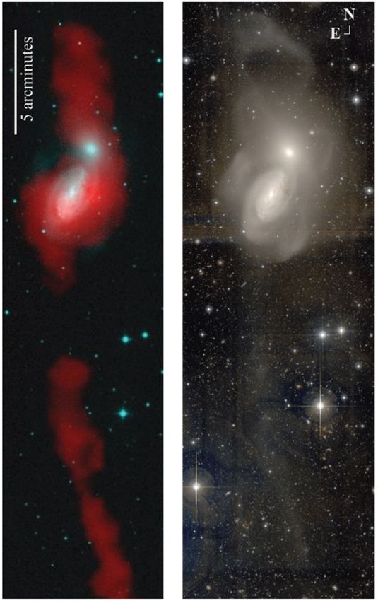
M. Querejeta et al.: ALMA resolves GMCs in a tidal dwarf galaxy

 N
 E
 40” ~ 2.8 kpc HI contours
 5 arcmin ~ 21 kpc

 extinction

 N

 S

 newborn stars

 10” ~ 700 pc

 deep optical HST WFC3 F547M
 composite g + r + H⍺ contours
 + HI

Fig. 1. Left panel: H i emission in the Arp 94 system (in red) on top of a deep optical image from Mundell et al. (1995b). Central panel: composite
g + r deep optical image from MegaCam/CFHT using an “arcsinh stretch” to emphasise faint emission (Duc et al. 2014). Both the left and central
panels come from Appleton et al. (2014). Top-right panel: blow-up of the g + r composite image showing the location of the TDG in H i emission
as blue contours, equivalent to an extinction of 0.4, 1.4, 2.4, and 3.4 AB magnitudes, ranging from 4 × 1020 to 4 × 1021 cm−2 (Mundell et al. 2004);
the annotations indicate the area where a high optical extinction is seen towards the background galaxy (north-east) and the star-forming region
in the south, as well as the demarcation line at Dec = 19◦ 510 5000 that we apply to distinguish the northern from the southern part of the TDG.
Bottom-right panel: star-forming region in the south of the TDG as revealed by young clusters visible in HST WFC3/F547M imaging and Hα
emission from Mundell et al. (2004) shown as contours (0.8, 2, 3, and 4 × 1033 erg s−1 pc−2 ).

 The full extent of the TDG (∼6400 × 4300 ) was covered with ferometric data. We also performed an alternative imaging of the
an 18-pointing mosaic by the 12 m array (primary beam of full interferometric data, combining the visibilities from the 12 m
width at half maximum FWHM = 25.300 ); a 7-pointing mosaic and 7 m arrays (without total power). In all cases, we cleaned
was sufficient to cover the same field of view with the 7 m array, using the Hogbom algorithm with natural weighting, down to
given the larger primary beam (FWHM = 43.500 ). In both cases, a threshold of 2 mJy per beam (∼2σ) in 2.5 km s−1 channels,
the mosaic was hexagonally packed, with approximate Nyquist and within the area where the primary beam response remains
sampling along rows (0.51× the primary beam) and a spacing higher than 20% of the maximum (which roughly corresponds
 √
 3/2 times the Nyquist separation between rows. to a tilted rectangle of ∼8000 × 7000 ≈ 5.6 × 4.9 kpc; shown
 We calibrated and imaged the datasets using CASA 5.4.1 as a dashed blue line in the left panel of Fig. 3). We chose a
(Common Astronomy Software Applications1 ). After standard pixel size of 0.08200 and an image size of 1344 × 1440 pixels
calibration, we concatenated the visibilities corresponding to the (centred on RA = 10:23:26.249, Dec = +19:51:58.83). With this
7 m and 12 m interferometric data and imaged them together. imaging strategy, we obtained an average synthesised beam of
We used the total power observations as model within tclean 0.6900 × 0.6000 (PA = 11◦ ), which corresponds to ≈45 pc for our
in CASA, so that the final cube recovers all the flux. The total assumed distance. The rms brightness sensitivity of the resulting
power data were calibrated and imaged following the strategy data cube is σrms ∼ 1 mJy per beam (≈56 mK), which for a rep-
presented in Herrera et al. (2020), Appendix A. For the baseline resentative linewidth of FWHM = 15 km s−1 yields a molecular
correction, we fitted a polynomial of order 1 in a fixed velocity gas surface density sensitivity of ∼3.9 M pc−2 (or a 1σ point-
window (755–855 km s−1 and 1500–1600 km s−1 ). We matched source sensitivity of ∼9 × 103 M ) for our assumed αCO con-
the spatial grid and spectral resolution (2.5 km s−1 ) of the inter- version factor (Sect. 2.4). In order to track flux recovery and
 compare against ancillary data, we also produced a version of
1
 http://casa.nrao.edu the final cube convolved to lower resolution (with a circular

 A97, page 3 of 20

A&A 645, A97 (2021)

Gaussian kernel of FWHM = 1.500 , 300 , and 6.300 , the latter to space and velocity. Thus, we constructed a Boolean mask for the
match the resolution of the H i data). We note that we did not main galaxy, isolating contiguous areas in the channel maps.
detect any continuum emission. We applied a primary beam cor- This mask was applied to the H i and CO cubes at full reso-
rection to the final cubes before performing any measurements. lution to exclude emission from NGC 3227.
All velocities in this paper are heliocentric, expressed following We obtained intensity maps for CO and H i emission by inte-
the radio convention (v = c(ν0 − ν)/ν0 ). grating the corresponding cubes, after applying the mask exclud-
 ing the emission from NGC 3227. We integrated in the velocity
 range [1060, 1360] km s−1 . We considered the velocity range
2.2. Ancillary data [1360, 1450] km s−1 as line-free and used those channels to esti-
2.2.1. VLA H i data mate the rms noise on a pixel-by-pixel basis. When computing
 moment maps, we applied a dilated mask technique to minimise
To trace atomic gas, we use H i observations from the Very Large the impact of noise (Rosolowsky & Leroy 2006); we started from
Array (VLA), originally published in Mundell et al. (2004). The a threshold of 4σ based on the rms map, and then dilated the
data were taken by the VLA in B configuration, with a spatial mask to include any adjacent voxels above 1.5σ. We used the
resolution of 6.300 and velocity resolution of 10 km s−1 . Previ- same dilated mask technique to construct first- and second-order
ously, Mundell et al. (1995b) had used the VLA to map the same moment maps. We obtained uncertainty maps for the first- and
target at lower resolution (∼2000 ) in C configuration. The amount second-order moment maps by formally propagating rmschannel .
of diffuse H i flux that is filtered out in B configuration is prob-
ably low, since the C array only recovered ∼12% more flux than 2.4. Conversion to gas surface densities
the B array (Mundell et al. 2004).
 To convert the ALMA CO(2–1) intensities into molecular gas
 surface densities, we applied a constant factor of αCO 2−1
 =
2.2.2. IRAM 30 m data −1 2 −1
 4.4 M (K km s pc ) , which is the average value measured
 by Sandstrom et al. (2013) directly on the CO(2–1) line for
We compare our CO(2–1) observations against previous CO(1–
 a set of resolved nearby galaxy discs (with a galaxy-to-galaxy
0) observations of the TDG with the IRAM 30 m telescope.
 scatter of 0.3 dex, implying fluctuations of a factor of ∼2). The
Those single-dish observations were published by Lisenfeld
 near-solar metallicity of the TDG suggests that this is proba-
et al. (2008), and they attained a spatial resolution of 2200 .
 bly a reasonable assumption. The constant α2−1 CO has the advan-
 tage that our surface density maps remain proportional to the
2.2.3. HST data directly measured CO(2–1) intensity. This value is equivalent to
 2 × 1020 cm−2 (K km s−1 )−1 when applied on the CO(2–1) line,
We make use of archival data from the Hubble Space Tele- including a factor of 1.36 to correct for the presence of helium.
scope (HST) taken with the Wide Field Camera 3 (WFC3). We The standard Galactic value is 2 × 1020 cm−2 (K km s−1 )−1
obtained the data covering both NGC 3227 and the TDG from when applied on the CO(1–0) line. Thus, considering the
the HST archive (proposal 11661, PI: Misty Bentz), which fol- mean CO(2–1)/CO(1–0) line ratio of 0.5−0.6 of this TDG (see
lows on-the-fly calibration procedures. The map was obtained Sect. 4.1.3), the fiducial molecular gas surface densities that we
with the medium-band filter F547M of the WFC3 camera and derive in this paper are ∼40−50% lower than what would be
has been presented in Batiste et al. (2017). We corrected the implied by the standard Galactic conversion factor applied on
astrometry of the HST image using Gaia field stars as ref- CO(1–0). In principle, we could also assume a spatially vary-
erence (a total of 15 stars down to 21 mag in g-band, Gaia ing α2−1
 CO , assuming a constant αCO modulated by the observed
 1−0

DR2; Gaia Collaboration 2016, 2018). The offsets applied were CO(2–1)/CO(1–0) ratio map. This would result in molecular gas
∆RA = 1.2 px (0.0500 ) and ∆Dec = −7.8 px (−0.3100 ). surface densities that are a factor ∼3 and ∼1.5 higher in the north
 and south, respectively. We prefer to avoid this modulation of
 αCO by R21 because of the coarse resolution (∼2800 ) of the avail-
2.2.4. Hα data
 able R21 map, limited by the CO(1–0) single-dish data.
We use Hα observations of NGC 3227 from the 4.2 m William We transformed H i intensities into atomic gas surface den-
Herschel Telescope in La Palma, presented in Mundell et al. sities using the standard formula for optically thin gas, ηH =
 1.82 × 1018 × FH i , where FH i is in K km s−1 and ηH is in atoms
(2004). We corrected the astrometry of the Hα image by apply-
 per cm2 (e.g. Condon & Ransom 2016). This is equivalent to
ing an offset of ∆RA = 0.33 px (0.1100 ) and ∆Dec = 2.05 px
 multiplying by 0.0145 to transform from K km s−1 to M pc−2 .
(0.6700 ) to match Gaia field stars.

 3. GMC identification and characterisation
2.3. Moment maps of the TDG emission
 3.1. GMC segmentation with CPROPS
As illustrated by Fig. 1, the TDG partially overlaps in pro-
jection with the background galaxy NGC 3227. To isolate the To perform the GMC identification with CPROPS (Rosolowsky
emission associated with the TDG from the emission arising & Leroy 2006), we started from a mask of significance defined
from NGC 3227, we followed a data-driven approach. Firstly, we as those voxels with signal above 4σ expanded to any adjacent
smoothed the H i cube to 3000 resolution in space and 50 km s−1 voxels with emission above 1.5σ. The same mask of signifi-
in velocity, boosting the signal-to-noise ratio. Then, we clipped cance was used for SCIMES (Colombo et al. 2015), as described
pixels below 3σsm , where σsm = 1 mJy beam−1 is the rms noise in Appendix A.2. Starting from the connected, discrete regions
per channel in the smoothed H i cube. In this clipped cube, the of signal within the mask (the so-called “islands”), local max-
H i emission from the main galaxy and that from the TDG can ima were subsequently identified and kept only if the voxels that
be unambiguously identified because they cover distinct areas in are closer to a given maximum than to any other maxima define

A97, page 4 of 20

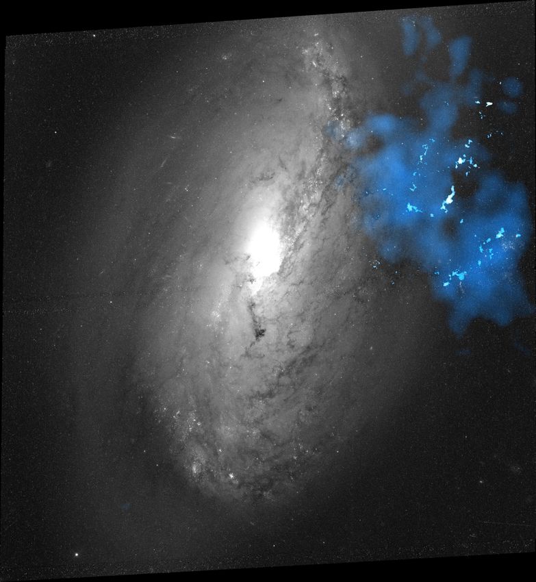
M. Querejeta et al.: ALMA resolves GMCs in a tidal dwarf galaxy

 with the major and minor axes of the cloud, determined from
 NGC 3227 2 kpc TDG principal component analysis. Subsequently, the size of the
 cloud was calculated as the intensity-weighted second moment
 (σmaj , σmin ) along each spatial dimension:
 sP sP
 i T i (yi − ȳ)
 T (x − x̄) 2 2
 i i i
 σmaj = P , σmin = P , (2)
 i Ti i Ti
 √
 with σr = σmaj σmin . The size of the cloud, R, was calculated
 as R = ησr , where η translates the spatial second moment to the
 radius of a spherical cloud, and it depends on the density distri-
 bution of the GMC. We adopted η = 1.91 (Solomon et al. 1987),
 which is the most standard assumption in Galactic and extra-
 galactic studies. When the cloud size provided by the segmenta-
 tion codes was smaller than the synthesised beam, the GMC was
 considered unresolved and was excluded from the analysis.
 Analogously, the velocity dispersion was obtained as:
 sP
 i T i (vi − v̄)
 2
 σv = , (3)
 HST-exposed
 P
 i Ti
 clusters √
 with the FWHM linewidth given by ∆v = 8 ln(2)σv .
 Starting from the basic properties above, we also derived
Fig. 2. False-colour image combining the CO(2–1) intensity from a number of indirect properties, including luminous and virial
ALMA (white), optical image from HST (greyscale), and H i intensity masses. The luminous mass was obtained as Mlum = αCO 2−1
 LCO ,
(blue) from the VLA (Mundell et al. 2004). The circles show a blow- while the virial mass was estimated as Mvir = 1040σv R (Mvir in2
up where HST reveals young stellar clusters associated with the star-
 M if σv is in km s−1 and R in pc), which assumes clouds with
forming part of the TDG.
 density profile ρ ∝ R−1 .
 To account for the effects of finite sensitivity, which can yield
an area larger than the synthesised beam. If this area was more slightly smaller GMC sizes than in reality, we used the extrapola-
than one synthesised beam but less than two beams, the island tion of the moments to the 0 K contour implemented in CPROPS
was included in the catalogue but not decomposed. Addition- and SCIMES (Rosolowsky & Leroy 2006). Additionally, the
ally, the local maxima must be 2σrms above the merge level with synthesised beam was deconvolved from the extrapolated spatial
other clouds. For all pairs of local maxima within an island, if moments. To account for uncertainties, we ran CPROPS with the
the computed moments based on the emission associated with bootstrap option, performing 1000 iterations.
each of the maxima separately differed less than 100% from the
moments computed for the combined emission, then those were
no longer considered as separate peaks. After this process, all the 4. Results
emission uniquely associated with a surviving local maximum Figure 2 shows the distribution of the molecular gas revealed by
was considered a segmentation unit (a GMC). ALMA (white) on top of atomic gas (blue) and stellar contin-
 We considered emission as long as the primary beam uum (greyscale). This composite-colour image already hints at
response from ALMA was at least 20% of the maximum, which some of the most important results of this paper. The H i obser-
corresponds to an area of ∼8000 ×7000 . We masked emission from vations at 6.300 resolution show that atomic gas extends over
the background galaxy NGC 3227 as described in Sect. 2.3. a relatively large projected area (∼6 kpc × 4 kpc = 24 kpc2 ). The
 ALMA observations at high-resolution (0.6400 ) reveal that the
3.2. Deriving GMC properties molecular emission that stands out on sub-arcsecond scales is
 highly clumpy and has a low covering factor. However, a very
We followed Rosolowsky & Leroy (2006) to extract physical large fraction of the molecular gas is diffuse; we examine this in
properties out of the discrete units identified by CPROPS and Sect. 4.1, together with the molecular-to-atomic gas ratio and
SCIMES. The quantities extracted by the segmentation codes are CO(2–1)/CO(1–0) ratio. We study the GMC properties, mass
the fluxes F, the sizes R, and the linewidths ∆V. spectra, and GMC scaling relations in Sect. 4.3. In Sect. 4.2 we
 Our ALMA cube can be characterised by a brightness tem- focus on gas kinematics. The clusters visible in Fig. 2 (high-
perature T i for each volumetric pixel (voxel i). Each voxel can lighted by the circular blow-ups) are often not aligned with the
also be identified by two spatial coordinates (xi , yi ) and a veloc- peaks of CO emission; we look at these offsets in Sect. 4.4.
ity channel (vi ); according to the segmentation, a given GMC
covers a discrete range of pixels and velocity channels (δx, δy,
δv). The luminosity was obtained adding up all emission within 4.1. Molecular structure of the TDG
the desired range of voxels: 4.1.1. Molecular-to-atomic gas ratio
 X
LCO = T i δx δy δv D2 , (1) The left and central panels of Fig. 3 show the CO and H i inten-
 i sity maps at matched 6.300 resolution, overlaid with CO contours.
where D is the distance to the galaxy. To obtain sizes, both There is plenty of CO emission where H i emission is very lim-
CPROPS and SCIMES first rotate the x and y axes to be aligned ited (below our detection threshold of 4σ), particularly towards

 A97, page 5 of 20

A&A 645, A97 (2021)

 H2 surface density (M☉/pc2) HI surface density (M☉/pc2) H2/HI surface density ratio
 0 3.5 7 10.5 14 4 8 12 16 0.40 0.80 1.20 1.60

 40"

 30"

 20"

 10"

 52' 00"

 50"

 40"

 30"
 beam beam
 20" 1 kpc
 1 kpc 1 kpc
 19o 51' 10"
 29s 28s 27s 26s 10h 23m 25s 28s 27s 26s 10h 23m 25s 28s 27s 26s 25s 10h 23m 24s

Fig. 3. Left panel: H2 surface density from ALMA CO(2–1) observations (12 m + 7 m + TP) convolved to 6.300 resolution, with contours highlight-
ing levels of (2, 6, 10) M pc−2 . The dashed blue line is the ALMA field of view (where the primary beam response exceeds 20%). Central panel:
H i surface density from the VLA at 6.300 resolution (Mundell et al. 2004), with CO contours from the left panel in red. Right panel: the ratio of
molecular-to-atomic gas surface densities derived from our CO(2–1) and H i observations (left and central panel) at 6.300 resolution; CO contours
as in the other two panels. In all maps north is up and east is left, with J2000.0 equatorial coordinates.

Table 1. Molecular and atomic gas properties at matched 6.300 tor of 2–3. In addition to local variations, globally the quiescent
resolution. north has a substantially higher molecular-to-atomic gas ratio
 (1.47) than the star-forming south (0.37). This becomes extreme
 Whole TDG North (a) South (b) in the north-west corner, where the ΣH2 /ΣH i ratio is at least ∼4−6
 Total H2 mass (M ) 8.6 × 107 7.3 × 107 1.3 × 107
 considering 4σ upper limits for H i. Averaging the local ΣH2 to
 Total H i mass (M ) 8.4 × 107 4.9 × 107 3.5 × 107 ΣH i ratio for pixels with simultaneous CO and H i detections
 Mean ΣH2 (M pc−2 ) 4.8 5.7 2.5
 results in a lower ratio than dividing the total H2 and H i masses.
 Mean ΣH i (M pc−2 ) 8.1 7.8 8.4 Independently from the indicator used, the molecular-to-atomic
 Total H2 mass/total H i mass 1.02 1.47 0.37
 gas ratio is surprisingly higher in the quiescent north, whereas
 Mean ΣH2 /ΣH i 0.59 0.73 0.30 star formation is enhanced in the more atomic gas-dominated
 Mean R21 = CO(2–1)/CO(1–0) 0.52 0.56 0.38
 south. The average H2 surface density is also higher in the north,
 while the average H i surface density is similar among both envi-
Notes. (a) North is where Dec > 19◦ 510 5000 . (b) South is where ronments. The molecular-to-atomic ratio remains higher in the
Dec < 19◦ 510 5000 . Measurements at matched spatial resolution (6.300 ) north even if we use a spatially variable α2−1
 CO (Sect. 2.4), but the
applying a mask of significance to both cubes (4σ dilated mask); thus, difference between north and south becomes smaller.
the total H2 mass quoted here is lower than implied by ALMA at native
resolution without any masking (1.6 × 108 M ). The mean ΣH2 and
ΣH i are calculated for pixels with significant detections of H2 and H i, 4.1.2. Diffuse molecular gas
respectively; this means that they are averaged over different areas.
 Table 2 provides the CO flux recovered by our observations
 using different ALMA arrays. Specifically, the 12 m array
the north-west of the TDG. The map also suggests that CO emis-
sion is somewhat clumpier than H i emission. Indeed, the stan- (configuration C40-4) and the compact 7 m array are sensitive
dard deviation in the flux distribution in the CO map (0.45 on a to scales up to 400 ∼ 280 pc and 2900 ∼ 2 kpc, respectively,
logarithmic scale) is almost twice higher than H i (0.25), con- while the combination of 12 m + 7 m + total power should cap-
firming that H i is more homogeneous even at matched reso- ture emission from all scales. Given the very low covering factor
lution. These effects contribute to the spatial variation of the of emission in the 12 m + 7 m cube, we applied a mask to ensure
molecular-to-atomic gas ratio evident in the right panel of Fig. 3: that we extract only meaningful flux (using a 4σ dilated mask
there are important changes in the H2 /H i ratio both locally as explained in Sect. 2.3). This mask encapsulates the compact
(around CO peaks) and globally (between the north and south structures that the 12 m + 7 m interferometer is sensitive to. We
of the TDG). measured the flux inside the same mask both for the 12 m + 7 m
 Table 1 lists our measurements of the molecular-to-atomic and 12 m + 7 m + TP cubes: the 12 m + 7 m cube recovers almost
gas ratio for the two environments in the TDG. Similar to other the whole flux (94%) in these compact structures. However, if
TDGs (Braine et al. 2001), this system is highly molecular with a we compare this compact emission against the total CO flux in
total H2 /H i mass ratio of ∼1. However, the molecular ratio varies the 12 m + 7 m + TP cube, almost 90% of the total CO flux is
significantly across the TDG with local variations up to a fac- outside the mask.

A97, page 6 of 20

M. Querejeta et al.: ALMA resolves GMCs in a tidal dwarf galaxy

Table 2. Fluxes (in K km s−1 kpc2 ) retrieved with or without short spacings and in GMCs at the native ALMA resolution (0.6400 ).

 Environment Area (kpc2 ) Flux in 12 m + 7 m + TP Flux in 12 m + 7 m Flux in GMCs (e)
 Inside mask (d)
 Total Inside mask (d)
 Whole TDG (a) 25.6 37.1 4.86 (13.1%) 4.58 (94.2%) 6.76 (18.2%)
 North (b) 15.8 28.5 3.93 (13.8%) 3.70 (94.1%) 5.44 (19.1%)
 South (c) 9.9 8.5 0.93 (10.9%) 0.88 (94.6%) 1.32 (15.5%)
Notes. (a) Whole TDG is the entire ALMA field-of-view, where the primary beam response exceeds 20% (dashed blue line in Fig. 3; ∼8000 × 7000 ).
(b)
 North is where Dec > 19◦ 510 5000 . (c) South is where Dec > 19◦ 510 5000 . (d) Flux inside 4σ dilated mask (the mask is identical in both cases and is
based on the 12 m + 7 m cube). The fourth and fifth columns indicate the percentage of the total 12 m + 7 m + TP flux that is inside the dilated
mask and the percentage of 12 m + 7 m + TP flux recovered with 12 m + 7 m inside the same mask, respectively. (e) Total flux in all GMCs identified
with CPROPS, after extrapolation to 0 K and deconvolution of the beam; without extrapolation and deconvolution, the total flux in GMCs is
considerably lower, 2.46 K km s−1 kpc2 . The percentage of the total 12 m + 7 m + TP flux is listed. The total flux in GMCs identified with SCIMES
(Appendix A.2) is 8.18 and 2.94 K km s−1 kpc2 for the extrapolated and non-extrapolated version, respectively.

 Extended emission can also be quantified as the fraction of by convolving the IRAM 30 m cube to 2800 resolution. Then,
the total CO flux that is contained in the GMCs identified by we computed the relevant moment-zero maps (Sect. 2.3) and
CPROPS (see Sect. 3.1). Depending on whether we include the took their ratio, CO(2–1)/CO(1–0), in flux units of K km s−1 .
extrapolation to infinite sensitivity or not, the flux in GMCs is The average value (masking NGC 3227) is 0.52, in good agree-
18% or 7% of the total, respectively. This roughly agrees with ment with the global R21 = 0.54 ± 0.10 found by Lisenfeld et al.
the amount of flux in compact structures that is captured by the (2008).
interferometer (12 m + 7 m data). Thus, most molecular emis- Figure 5 shows that there is a significant gradient in R21 along
sion is not arising from the type of compact structures that are the TDG, from a maximum of ∼0.7 in the north down to a min-
responsible for massive star formation in galaxies. The extended imum of ∼0.3 in the south. This might indicate changes in the
emission is likely associated with diffuse molecular gas, and physical properties of molecular gas between the quiescent and
it accounts for as much as ∼80−90% of the molecular emis- star-forming part of the TDG. We also computed R21 for the part
sion in the TDG. This is substantially higher than the values of the background galaxy NGC 3227 simultaneously covered by
found in other nearby galaxies (typically 10–60%; Pety et al. the ALMA and IRAM 30 m observations. In NGC 3227, we find
2013; Caldú-Primo et al. 2015), only comparable to the 74−91% an average value of 0.53, similar to the global ratio for the TDG.
extended emission found in the bar of NGC 1300 (Maeda et al. In Sect. 5.2 we discuss how the mean R21 ratio in the TDG is
2020b). There is no strong dependence of the diffuse fraction on compatible with the lowest values observed in nearby galaxies.
environment: it is slightly higher in the north but quite similar in
both cases (see Table 2). 4.2. Kinematics
 Figure 4 shows the spatial distribution of compact CO emis-
sion at 6.300 resolution (ALMA 12 m + 7 m data, without total The H i emission shows a clear velocity gradient along the north-
power) against the diffuse component (the result of subtracting south direction which was interpreted by Mundell et al. (2004)
 as possibly due to rotation. The left panel of Fig. 6 shows the dif-
the intensity from ALMA 12 m + 7 m + TP minus the intensity
 ference between the moment-1 maps for H i and CO at matched
from 12 m + 7 m only, channel by channel). We performed this 6.300 resolution. There are significant velocity offsets towards
analysis at 6.300 resolution to avoid being dominated by local some regions in the north (up to ∼100 km s−1 ). Conversely, there
spikes due to noise, and because it is the resolution of the H i is reasonably good agreement between CO and H i velocities
map. As expected, the diffuse component is smoother than the towards the south (mostly within ±20 km s−1 ).
compact emission even at matched 6.300 resolution. Yet, the dif- The middle and left panel of Fig. 6 focus on the highest res-
fuse emission is not perfectly homogeneous either, and seems to olution available from ALMA. These high-resolution moment
be more intense towards the north. maps show differences with H i since the CO peaks seem to be
 The diffuse component shows a north-south velocity gradient organised into several kinematically coherent filaments. Rather
and, as one might expect, the velocity in diffuse CO varies more than a smooth gradient, there are quite abrupt changes in the
smoothly than in compact CO structures. The CO linewidth is velocities of these filaments. This could be indicating that the
high (σ ∼ 50−60 km s−1 ), and correlates with intensity. This is high-density interstellar medium (ISM) is made up of relatively
in stark contrast with the compact component, which shows large independent sub-structures, embedded in a more diffuse molec-
local variations in velocity and linewidth, as well as much more ular medium.
limited velocity dispersion (mostly below ∼20−30 km s−1 ). The Figure 7 shows position-velocity diagrams of H i along the
kinematics of the compact component does not follow in detail three slits indicated in Fig. 6. Simultaneously, we track as red
the velocity field and dispersion map of the diffuse component. contours the diffuse CO emission at a matched resolution of 6.300
 (i.e. the emission that is filtered out by the interferometer, like
4.1.3. CO(2–1)/CO(1–0) ratio the bottom panels of Fig. 4). To first-order approximation, there
 is very good agreement between the atomic gas and diffuse CO,
mnus 1ptWe explore spatial variations in R21 by combining our and they both reflect the north-south velocity gradient seen at
ALMA total power CO(2–1) observations (2800 resolution) with lower resolution. There are two noteworthy differences, though:
the IRAM 30 m CO(1–0) single-dish observations (2200 resolu- (1) in the NE ridge, there is plenty of diffuse CO at low veloci-
tion) from Lisenfeld et al. (2008). We first matched resolutions ties (∼1050−1150 km s−1 ) where the VLA cube did not register

 A97, page 7 of 20

A&A 645, A97 (2021)

 Moment 0 intensity (K km/s) Moment 1 velocity (km/s) Moment 2 velocity disp. (km/s)
 0 0.6 1.2 1.9 2.5 1100 1150 1200 1250 1300 0 15 30 45 60

 40"
 1 kpc 1 kpc 1 kpc
 Compact CO(2-1) emission

 30"

 20"

 10"

 52' 00"

 50"

 40"

 30"
 beam beam beam
 19o 51' 20"

 40"

 30"
 Diffuse CO(2-1) emission

 20"

 10"

 52' 00"

 50"

 40"

 30"

 beam beam beam
 19o 51' 20"

 29s 28s 27s 26s 25s 10h 23m 24s 28s 27s 26s 25s 10h 23m 24s 28s 27s 26s 25s 10h 23m 24s

Fig. 4. Top panels: compact emission traced by the ALMA 12 m + 7 m arrays without TP. Bottom panels: diffuse molecular emission obtained by
subtracting the compact emission channel by channel (top panels) from the total molecular emission measured by ALMA 12 m + 7 m + TP (i.e.
including short spacings): this is the emission that is filtered out by the interferometer. Left panels: zeroth-order moment maps, measuring the
integrated intensity (in K km s−1 ). Middle panels: first-order moment maps, representing the velocity field (in km s−1 ). Right panels: second-order
moment maps, tracing CO linewidths (σ in km s−1 ). In all panels, the grey circle in the bottom right represents the FWHM of the synthesised beam
(6.300 ).

 53' 00" 0.70 around regions of enhanced H i emission, except in the NE
 ridge, where most GMCs are offset from H i by ∼50−150 km s−1
 50"
 towards lower velocities. There is diffuse CO emission coincid-
 40" ing with or near those offset GMCs, but almost no significant
 0.60
 H i visible (some diffuse, faint H i emission is however visible
 30"
 in a deeper cube from the C-array of the VLA; Mundell et al.
 1995b). This offset towards lower velocities is suggestive of an
 CO(2-1) / CO(1-0)

 20"
 overlap of gaseous structures along the line of sight: the dis-
 10" tribution of diffuse emission and GMCs is rather continuous,
 0.50
 52' 00"
 starting from the main H i emission around ∼1200−1300 km s−1
 and extending towards velocities closer to the disc of NGC 3227
 50" (∼1000 km s−1 ). This may indicate that a gaseous bridge con-
 nects the TDG with the background spiral galaxy. The clustering
 40"
 0.40 of clouds at lower velocities can be well visualised through a
 30" rotating position-position-velocity representation of the GMCs
 beam which is available online.
 20"
 1 kpc Another important issue from the kinematic point of view
 0.30
 19o 51' 10" is the higher CO velocity dispersion found in the north of the
 29s 28s 27s 26s 25s 24s 10h 23m 23s TDG compared to the south. Lisenfeld et al. (2008) suggested
 that this might reflect an increase in large-scale turbulence in
Fig. 5. CO(2–1)/CO(1–0) ratio at 2800 resolution.
 the north that might, in turn, prevent gas from forming stars
 in that part of the TDG. Taking the velocity centroid from
significant H i emission; (2) there is an offset of ∼30 km s−1 each GMC (Sect. 4.3), we computed the statistical dispersion
between H i and diffuse CO in the star-forming ridge in the south. of those velocities for the ensemble of clouds in the north and
 We can also examine the distribution of GMCs (Sect. 3) on in the south. Within GMCs, the intrinsic velocity dispersions are
the position-velocity diagrams of Fig. 7. GMCs tend to cluster slightly higher in the north (median σGMC ∼ 6.5 km s−1 ) than in
A97, page 8 of 20

M. Querejeta et al.: ALMA resolves GMCs in a tidal dwarf galaxy

 CO-HI velocity diff. (km/s) Moment 1 velocity (km/s) Moment 2 velocity disp. (km/s)
 -100 -70 -40 -10 20 1100 1150 1200 1250 1300 0 6 12 18 24

 40"
 NE NW
 30"

 20"

 10"

 52' 00"

 S
 50"

 40"

 30"
 beam
 20" 1 kpc
 1 kpc 1 kpc
 beam beam beam
 19o 51' 10"
 29s 28s 27s 26s 10h 23m 25s 28s 27s 26s 25s 10h 23m 24s 28s 27s 26s 25s 10h 23m 24s

Fig. 6. Left panel: difference between moment-1 maps for CO (ALMA 12 m + 7 m + TP) and H i at matched 6.300 resolution. Middle panel: CO
velocity field at 0.6400 ≈ 45 pc resolution measured as the moment-1 map from ALMA (12 m + 7 m + TP), using a 4σ dilated mask. The blue
arrows are the slits used for the position-velocity diagrams from Fig. 7. Right panel: CO velocity dispersion measured as the moment-2 map from
ALMA (12 m + 7 m + TP), using the same 4σ dilated mask.

 1400
 NE NW S
 1300
 velocity (km/s)

 1200

 1100 Background: HI
 Contours: diffuse CO
 Circles: GMCs
 1000
 -20" 0 20" -20" 0 20" -20" 0 20"
 offset along slit (") offset along slit (") offset along slit (")
Fig. 7. Position-velocity diagrams of H i (at 6.300 resolution) in greyscale and black contours along the three slits indicated in Fig. 6. Red contours
show the distribution of diffuse CO emission from ALMA (12 m + 7 m + TP minus 12 m + 7 m only), corresponding to 6, 9, 12 mK. Blue circles
indicate the location of GMCs identified with CPROPS.

the south (σGMC ∼ 4.5 km s−1 ), and the relative cloud-to-cloud SCIMES (Colombo et al. 2015), a dendrogram-based method
velocity dispersion is also higher in the north (σcloud−cloud ∼ (Rosolowsky et al. 2008) which, on top of segmenting the molec-
73 km s−1 ) than in the south (σcloud−cloud ∼ 46 km s−1 and as low ular ISM, informs on how it is hierarchically structured. In both
as 16 km s−1 if restricted to the star-forming area). cases, we follow the same strategy to derive physical proper-
 ties (Sect. 3.2). The results for the cloud ensemble derived using
 CPROPS and SCIMES are very similar, and that is why we
4.3. GMC properties and scaling relations
 focus on CPROPS next, while we point the interested reader to
The exquisite resolution of ALMA (0.6400 ≈ 45 pc) allowed us Appendix A.2 for the details on SCIMES. The final catalogue of
to resolve large and intermediate-size GMCs in this system, with GMC properties from CPROPS is presented in Table A.3.
molecular gas masses ranging from ∼104 M to ∼106 M . We
estimated our 5σ completeness limit as 5 × 104 M based on the
 4.3.1. GMC properties
point-source sensitivity derived in Sect. 2.1.
 We employed the CPROPS algorithm to identify GMCs We find a total of 111 GMCs with CPROPS (out of which 81
(Rosolowsky & Leroy 2006), as described in Sect. 3.1. In have extrapolated and deconvolved values), and Fig. 8 shows
Appendix A.2 we also present an alternative approach using their distribution, sizes, and orientation. Far from clustering

 A97, page 9 of 20

A&A 645, A97 (2021)

mostly towards the star-forming south (19 clouds), the number H2 surface density (M☉/pc2)
of GMCs is larger in the north (62 clouds), even though the pro-
 0 20 40 60 80
jected area in the north is only ∼50% larger. As expected, the dis-
tribution of GMCs follows the areas of strongest CO emission.
Some GMCs are rounder (axis ratio ∼1) while others are more 40"
elongated (∼3), and reassuringly we find no correlation between
the orientation of the GMCs and the PA of the ALMA synthe- 30"
sised beam.
 Table 3 summarises the typical properties of the GMCs. We
 20"
find GMCs with radii of a few tens of parsec (up to ∼100 pc),
luminous masses ranging ∼104 to ∼106 M , and velocity disper-
sions of a few km s−1 . These values are comparable to massive 10"
GMCs in the Milky Way and other nearby galaxies (e.g. Bolatto
et al. 2008; Heyer et al. 2009; Colombo et al. 2014; Faesi et al. 52' 00"
2018), in spite of the starkly different nature of the TDG. Virial
masses are larger than luminous masses, as we discuss later.
 50"
 We find no significant differences between global properties
of GMCs in the north and south of the TDG other than ∼50%
higher σv and Mvir in the north (Table 3). We confirmed that 40"
these results do not change qualitatively if we rely on the seg-
mentation from SCIMES instead of CPROPS (Table 3). 30"
 1 kpc beam
4.3.2. GMC mass spectra 19o 51' 20"
 29s 28s 27s 26s 10h 23m 25s
The GMC mass spectrum is an indicator of GMC formation and
dispersal timescales, modulated by mechanisms such as feed- Fig. 8. GMC positions and orientations indicated on the ALMA
back and cloud-cloud collisions, and it is expected to depend CO(2–1) integrated intensity map. GMCs are shown as ellipses with
on environment (Inutsuka et al. 2015; Dobbs et al. 2015; Torii the CPROPS extrapolated and deconvolved major and minor axes (2nd
et al. 2015; Kobayashi et al. 2017). Shallower GMC mass spec- moment of emission). Orange and blue ellipses represent clouds in
tra imply a higher proportion of massive clouds within a given the north and south of the TDG, respectively. The bottom-right corner
population; we denote the slope of the mass spectrum as γ. shows the ALMA synthesised beam (0.6900 × 0.6000 with PA = 11◦ ).
 Our completeness limit of 5 × 104 M is deeper than the
PAWS survey in M51 (3.6 × 105 M ; Colombo et al. 2014),
 We fitted both a truncated and non-truncated power law and
but not as deep as the study of Faesi et al. (2018) in NGC 300
 found that the truncated version applies better to our data. Con-
(8 × 103 M ). This means that the smallest clouds may be unre-
 sidering all GMCs in the TDG simultaneously (111 clouds), we
solved and blending is likely for some.
 find a slope of γ = −1.76 ± 0.13. This value is compatible
 To compare with GMC mass spectra in other galaxies, here with the slope of the GMC mass spectrum in the inner Milky
we focus on CPROPS, which is more widely used than SCIMES Way, where Rice et al. (2016) found γ = −1.59 ± 0.11; for
(shown in Appendix A). Unlike for GMC scaling relations, here the first Galactic quadrant, Colombo et al. (2019) also found a
we consider all the clouds identified by CPROPS (82 in the north fully compatible value, γ = −1.76 ± 0.01. Similar values have
and 29 in the south), as they all have extrapolated luminosities been found in M31 (γ = −1.63 ± 0.2; Rosolowsky 2007); in
that permit to derive total masses (MGMC = α2−1 CO LCO ). Rather M33 (γ ∼ −1.6 ± 0.2; Gratier et al. 2012; Braine et al. 2018);
than a binned histogram (differential form), we fitted a cumula- in the molecular ring and density-wave spiral arms in M51
tive mass distribution, which has been argued to be more robust (γ = −1.63 ± 0.17 to γ = −1.79 ± 0.09; Colombo et al. 2014);
in the case of small samples (Rosolowsky 2005) and its use is or in NGC 300 (γ = −1.76 ± 0.07; Faesi et al. 2018). Higher
more extended. When the cumulative GMC mass spectrum is values have been reported in some cases: the outer Milky Way
well described by a power law, it can be expressed by the fol- (γ = −2.1 ± 0.2; Rosolowsky 2005); the LMC (γ = −2.33 ± 0.16;
lowing formula: Wong et al. 2011); in the outer M33 (γ = −2.3 ± 0.2; Gratier
 !γ+1 et al. 2012); in the material arm and the interarm region in M51
 M
N(MGMC > M) = , (4) (γ = −2.44 ± 0.40 to γ = −2.55 ± 0.23; Colombo et al. 2014);
 M0 in the lenticular galaxy NGC 4526 (γ = −2.39 ± 0.03; Utomo
 et al. 2015); and in the strongly barred spiral NGC 1300 (γ =
where M0 is some reference mass (normalisation factor) and γ is
 −2.20 ± 0.04; Maeda et al. 2020a). Tosaki et al. (2017) found a
the slope of the power law.
 somewhat lower slope for GMCs in NGC 1068, γ = −1.25±0.07,
 Generally, the GMC mass spectrum can be better described
 similar to the value derived by Colombo et al. (2014) along the
as a truncated power law:
 nuclear bar of M51 (γ = −1.33 ± 0.21). All of these studies used
  M γ+1
  !  the cumulative version of the mass spectrum, which should make
N(MGMC > M) = N0  − 1 ,
 
  (5) the results comparable, but we note that Gratier et al. (2012) used
 M0 a different algorithm to fit the cumulative mass distribution and,
 in general, differences in the detailed cloud segmentation strate-
where N0 is the number of clouds more massive than 21/(γ+1) M0 , gies can affect the derived slopes.
the truncation mass where the distribution deviates from a power We also checked the difference between the GMC mass spec-
law. trum in the quiescent north and in the star-forming south of the
A97, page 10 of 20

M. Querejeta et al.: ALMA resolves GMCs in a tidal dwarf galaxy

Table 3. GMC properties as derived by CPROPS.

Property Unit TDG north south
 Min Median Max Min Median Max Min Median Max
T max K 0.3 0.4 1.0 0.3 0.4 0.8 0.3 0.5 1.0
LCO K km s−1 pc2 1.8 × 103 3.9 × 104 4.5 × 105 1.8 × 103 4.1 × 104 4.5 × 105 3.7 × 103 3.5 × 104 1.6 × 105
R pc 12.3 58.0 123.4 12.3 59.7 123.4 15.8 58.0 102.5
σv km s−1 0.9 5.8 19.7 0.9 6.6 19.7 0.9 4.5 9.1
Mlum M 8.1 × 103 1.7 × 105 2.0 × 106 8.1 × 103 1.8 × 105 2.0 × 106 1.6 × 104 1.5 × 105 7.0 × 105
Mvir M 2.3 × 104 2.7 × 106 4.0 × 107 2.8 × 104 3.4 × 106 4.0 × 107 2.3 × 104 2.3 × 106 7.8 × 106

 1 correlation coefficients are listed in Table 4. The linear regres-
 North South sions are obtained with two different methods. The first one is
 = -1.76±0.15 = -1.30±0.19 the popular orthogonal distance regression (ODR), where the
 data are fitted in the log-log plane using the Python implemen-
 log (NGMC | M > m)

 0
 tation scipy.odr2 that considers uncertainties in both variables
 completeness limit

 completeness limit

 simultaneously. As a complementary approach, we also fitted the
 observations using the publicly available Bayesian fitting code
 -1 BayesLineFit3 (Lelli et al. 2019) that additionally considers
 the intrinsic scatter along the relation. BayesLineFit provides
 similar results as the ODR method but larger uncertainties (from
 -2 exploring the full posterior distribution of the free parameters).
 3 4 5 6 4 5 6 In both cases, these fits are based on the extrapolated and decon-
 log (M/M☉) log (M/M☉)
 volved GMC properties (see Sect. 3.2), which result in substan-
Fig. 9. Cumulative GMC mass distribution for the two environments tially higher error bars; for instance, the median uncertainty on
in the TDG: north (left) and south (right). The vertical dashed lines the cloud radius is 18%, but as much as 55% when considering
indicate our completeness limit of 5 × 104 M . extrapolation and deconvolution.
 Size-linewidth relation. A power-law relationship between
TDG. Interestingly, we found that the south has a shallower mass size and velocity dispersion of GMCs has been systematically
spectrum, γ = −1.30 ± 0.19 instead of γ = −1.76 ± 0.15. The found in the Milky Way, with a slope of ∼0.5, which has been
difference is marginally significant given the large error bars interpreted as a manifestation of compressible turbulence within
(due to the relatively low number of clouds in each environ- the molecular ISM (e.g. Solomon et al. 1987; Heyer et al. 2001;
ment), but it points at an interesting idea: the higher proportion Rice et al. 2016; Kritsuk et al. 2017). Observations of the Galac-
of more massive clouds in the south might be connected with the tic central molecular zone imply a slightly steeper size-linewidth
star formation activity in that region. This would be consistent relation with a slope of ∼0.7 (Shetty et al. 2012; Kauffmann et al.
with similar observations in star-forming rings or spiral arms in 2017). The clouds in the TDG seem to have a moderate degree
nearby galaxies, where shallower GMC mass spectra correlate of correlation in this plane (left panel of Fig. 10), but the slope
with more intense star formation (Colombo et al. 2014; Tosaki γ = 2.00 ± 0.33 is significantly steeper than the canonical Galac-
et al. 2017). tic value of ∼0.5. If we subdivide clouds into our two environ-
 Another relevant quantity is the truncation mass of the GMC ments, we find a steeper slope for the north, but the difference is
mass spectrum. Fitting all GMCs in the TDG, we found a value only marginally significant given the large error bars.
of M0 = 1.9 × 106 M . While M51 shows a significantly higher Within the extragalactic literature, there is some controversy
truncation mass (∼2 × 107 M ; Colombo et al. 2014), M0 in the as to whether a genuine size-linewidth relation holds. Bolatto
TDG is of the same order as the LMC, NGC 4526, NGC 300, or et al. (2008) combined data from several nearby galaxies and
some Galactic results (M0 ∼ 1−4 × 106 M ; Wong et al. 2011; found evidence for a size-linewidth relation (γ = 0.60 ± 0.10).
Utomo et al. 2015; Rice et al. 2016; Faesi et al. 2018; Colombo On the other hand, a number of studies found that their data did
et al. 2019). These values agree with theoretical models for max- not support the existence of a size-linewidth relation (e.g. Gratier
imum cloud masses by Reina-Campos & Kruijssen (2017). et al. 2012 in M33; Colombo et al. 2014 in M51; Hughes et al.
 2013a combining M33, the LMC, and M51), or only weakly
 (e.g. Braine et al. 2018 in M33). More recently, Faesi et al.
4.3.3. GMC scaling relations (2018) found a size-linewidth relation in NGC 300 with a slope
Here we focus on a widespread GMC diagnostics tool: the of 0.48 ± 0.05, with a larger dynamic range in GMC masses than
Larson scaling relations, shown in Fig. 10. Larson (1981) and the previous studies. Our data have a similar degree of corre-
Solomon et al. (1987) found a tight correlation between the size lation as found by Faesi et al. (2018) in NGC 300 (they quote
and linewidth of GMCs, between their virial and luminous mass, a Pearson coefficient rP = 0.55). However, the substantially
and between their size and mass. Those seminal papers exam- steeper slope of the size-linewidth relation in the TDG suggests
ined Galactic GMCs, but more recent work has expanded the
analysis to extragalactic clouds as well. We focus on CPROPS 2
 https://docs.scipy.org/doc/scipy/reference/odr.html
 3
to minimise discrepancies with studies from the literature due to BayesLineFit is available at http://astroweb.cwru.edu/
different segmentation codes. The best fits and Spearman rank SPARC/

 A97, page 11 of 20