Chasing Government Jobs: How Aggregate Labor Supply Responds to Public Sector Hiring Policy in India - Harvard University
←
→
Page content transcription
If your browser does not render page correctly, please read the page content below
Chasing Government Jobs: How Aggregate Labor

   Supply Responds to Public Sector Hiring Policy in

                                              India

                                                              *
                                       Kunal Mangal
                                     (Job Market Paper)

                             This Version: April 4, 2021
                              Latest Version: click here

                                             Abstract
          Many countries allocate government jobs through a system of highly competitive
      exams.   For example, in India, civil service exams regularly attract over a half a
      million applications, with an acceptance rate of less than 0.1%. This paper studies
      whether the intense competition for these jobs aects aggregate labor supply. To
      answer this question, I study how the labor market responded to a civil service hiring
      freeze in the state of Tamil Nadu.     I nd that candidates responded by spending
      more time studying, not less. A decade after the hiring freeze was lifted, the cohorts
      that were most impacted also have lower earnings, suggesting that participation in
      the exam process did not build human capital.         Finally, I provide evidence that
      structural features of the testing environmentsuch as how well candidates are able
      to forecast their own performance, and the underlying returns to study eorthelp
      explain the observed response. Together, these results indicate that public sector
      hiring policy has the potential to move the whole labor market.

   * PhD candidate in Public Policy at Harvard University. Email: kmangal@g.harvard.edu. I am grateful
to my advisors Emily Breza, Asim Khwaja, and Rohini Pande for their support.        Robert Townsend
provided much appreciated initial encouragement. Kranti Mane provided outstanding research assistance.
I also thank Augustin Bergeron, Shweta Bhogale, Michael Boozer, Nikita Kohli, Tauhidur Rahman, Sagar
Saxena, Utkarsh Saxena, Niharika Singh, Perdie Stilwell, Nikkil Sudharsanan, and seminar participants
at Harvard for thoughtful discussions and comments. This work would not have been possible without
the support of K. Nanthakumar and S. Nagarajan of the Tamil Nadu Government, the sta at the R&D
Section of TNPSC, and Dr. Anand Patil and Mrs. Vaishali Patil in Maharashtra. I am also grateful to
the many candidates for government jobs who were willing to take the time to share their world with
me. Of course, any errors are my own. All human subjects data collection has been approved by the
Harvard University IRB.

                                                  1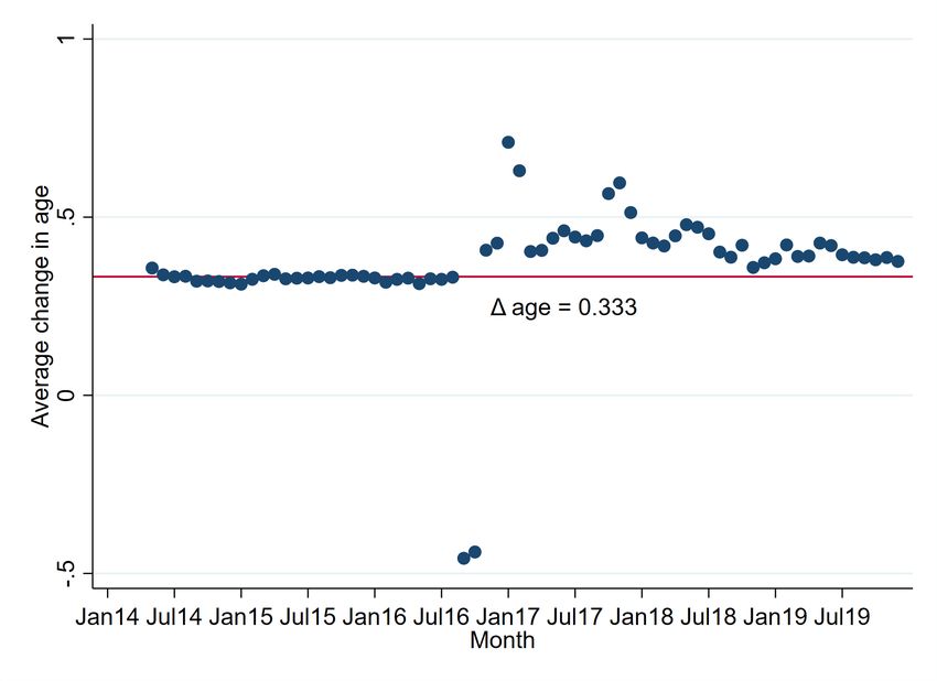
1 Introduction
Government employees in developing countries tend to enjoy substantial rents: not only
are wages typically higher than what comparable workers would earn in the private sector,
but these jobs also come with many valuable and rare amenities, such as lifetime job
1
security.
What costs do these rents impose on the rest of the economy? A key concern is
that rents could induce losses orders of magnitude larger than the
scal costs, due to
behavioral responses. Many countries have been particularly sensitive to the possibility
that the competition for rents will lead to the selection of less quali
ed candidates, either
due to patronage or bribery, and have responded by implementing rigid systems of civil
service exams, in which selection is based on objective, transparent criteria.
Although competitive exams usually succeed in minimizing political interference in
2
the selection process, economists have long been concerned that they do not fully mit-
igate the costs of rent-seeking behavior. In particular, one worries that the prospect of
a lucrative government job encourages individuals to divert time away from productive
3
activity towards unproductive preparation for the selection exam. However, it is un-
4
clear whether enough candidates respond in this way to aect the aggregate economy;
and it is possible that the eect may even be positive, if studying for the exam builds
5
general human capital. Thus, it is still an open question whether rent-seeking through
1 Finan, Olken, and Pande (2017) show that public sector wage premia decline with GDP per capita.
Wage premia likely understate the ex-post rents that government employees enjoy because of the ameni-
ties.
2 For example, Colonnelli, Prem, and Teso (2020) show that connections generally matter for selection
into the Brazilian bureaucracy, but not for positions that are
lled via competitive exam.
3 This exact concern has found mention in the literature from Krueger (1974) to, more recently,
Muralidharan (2015) and Banerjee and Du
o (2019). There are other potential costs which I do not
address in this paper. For example, another strand of the literature discusses how these rents could
starve the private sector of talented individuals, which would in turn aect aggregate productivity and
investment (Murphy, Shleifer, and Vishny, 1991; Geromichalos and Kospentaris, 2020).
4 A competitive exam is a tournament, and tournament theory predicts that only candidates on the
margins of selection should be responsive to the prize amount (Lazear and Rosen, 1981).
5 An increase in general human capital is just one potential social bene
t of exam preparation. For
example, learning about how government works (which is a commonly found on the syllabus of these
exams) might create more engaged citizens, who have a stronger belief in democratic ideals or who
2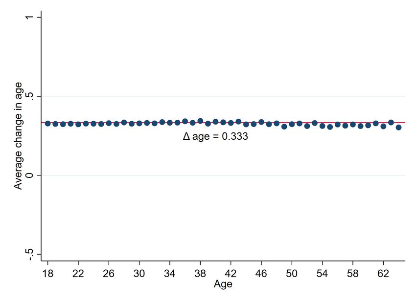
competitive exams imposes meaningful social costs.
In this paper, I provide, to my knowledge, the
rst empirical evidence on how the
competition for rents through the competitive exam system aects the rest of the economy.
I address three related questions: First, do rents in the public sector aect individuals'
labor supply decisions? Second, are investments in exam preparation productive in the
labor market, or are they mostly unproductive signaling costs? And
nally, what factors
aect how individuals respond to the availability of rents?
To answer these questions, I study the labor market impact of a partial hiring freeze in
the state of Tamil Nadu in India. India is a country where rents in public sector employ-
6
ment are particularly large, and where competitive exams are commonplace. In 2001,
while staring down a
scal crisis, the Government of Tamil Nadu suspended hiring for
most civil service posts for an inde
nite period of time. The hiring freeze was ultimately
lifted in 2006. Although civil service hiring fell by 85% during this period, because these
jobs constitute a small share of the overall government hiring, the hiring freeze had a
7
negligible impact on aggregate labor demand. Thus, how the labor market equilibrium
shifted during the hiring freeze tells us how labor supply responded, which in turn helps
us better understand the nature of the competition for rents in the civil service.
My analysis draws on data from nationally-representative household surveys, govern-
ment reports that I digitized, and newly available application and testing data from the
government agency that conducts civil service examinations in Tamil Nadu. I focus on
college graduates, who are empirically the demographic group most likely to apply for
civil service positions. To identify the impact of the hiring freeze, my main results use a
dierence-in-dierences design that compares: i) Tamil Nadu with the rest of India; and
ii) exposed cohorts to unexposed cohorts. For identi
cation, I rely on the fact that the
are better able to advocate for themselves and others. This paper will not be able to speak to those
considerations.
6 In the sample of 32 countries that Finan et al. (2017) include in their cross-country comparison,
India has the largest (unadjusted) public sector wage premium, both in absolute terms, and relative to
its GDP per capita. Consistent with government employees enjoying rents, surveys of representative
samples of Indian youth consistently
nd that about two-thirds prefer government employment to either
private sector jobs or self-employment (see Appendix Figure A.1). Among the rural college-educated
youth population, the preference for government jobs stands at over 80% (Kumar, 2019).
7 See Appendix B for details.
3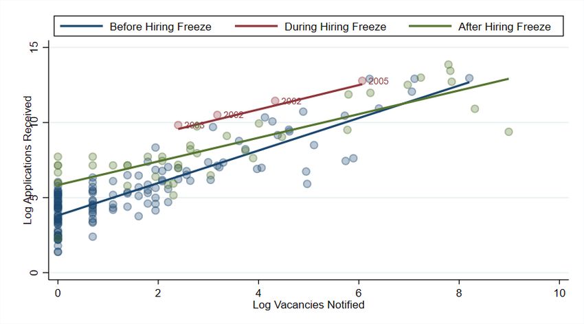
college graduation rates of men remain stable across cohorts. Unfortunately, because the
8
same is not true of women, I restrict the sample to men.
First, I show that aggregate labor supply does in fact respond to the availability of
government jobs. Using data from the National Sample Survey, I
nd that men who
were expected to graduate from college during the hiring freeze are 30% more likely to
be unemployed in their 20s than men in cohorts whose labor market trajectories were
measured before the start of the hiring freeze. The increase in unemployment corresponds
to a nearly equal decrease in employment rates.
Why are fresh college graduates more unemployed? The most likely answer is that
candidates spent extra time preparing for the competitive exam. During the hiring freeze,
the application rate for civil service exams skyrocketed to 10-20 times its normal rate.
It is unlikely, then, that college graduates responded to the hiring freeze by seeking
employment in the private sector instead.
If college graduates spent more time preparing for the exam, did they build general
human capital in the process? My next set of results suggest that the answer is no. If
exam preparation builds general human capital, we should expect to see higher labor
market earnings in the long-run among cohorts that spent more time preparing. To
test this hypothesis, I use data from the Consumer Pyramids Household Survey, which
measures labor market earnings about a decade after the hiring freeze ended. I
nd that, if
anything, earnings declined among those cohorts that spent more time in unemployment.
Lastly, I try to understand why candidates responded the way they did. I focus on how
the testing environment shapes the incentives for applicants in a way that helps explain
their response. There are at least two aspects to the response that we observe that are
puzzling. First, it is unclear why candidates were willing to spend more time studying
when the probability of obtaining a civil service job declined (at least in the short run).
Second, given that the hiring freeze did not have a de
nite end date, it is unclear why
candidates did not take up private sector jobs until the uncertainty was resolved.
To answer the
rst question, I propose that candidates are generally over-optimistic
8 Women are well-represented among civil service exam applicants in Tamil Nadu. Between 2012 and
2016, women represented 49% of all applicants in competitive exams for state-level jobs in Tamil Nadu.
4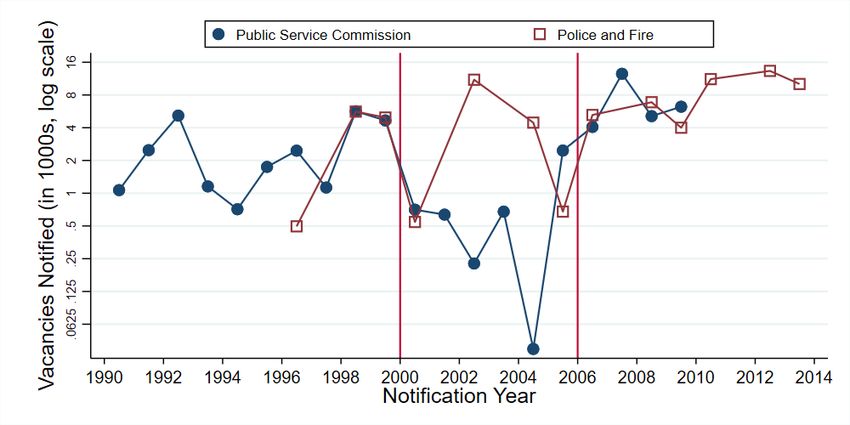
about their own probability of selection, and only revise their beliefs downwards through

the process of making attempts. I provide suggestive evidence to support this hypothesis.

I rst show that candidates are generally over-optimistic about their exam performance,

drawing on an incentivized prediction task I conducted with 88 civil service aspirants in

Maharashtra, a state with a similar civil service examination system as the one in Tamil

Nadu.      Next, using civil service exam application and testing data from between 2012

and 2016 in Tamil Nadu, I show that candidates respond to prior test scores when de-

ciding whether to make re-application decisions. A key empirical challenge in estimating

this relationship is that re-application decisions may be endogenous to ability. I therefore

draw from Item Response Theory, a branch of psychometrics, to construct an instrument.

The instrument isolate the luck" component of the test score from variation in ability.

Consistent with candidates learning about ability, I show that this luck component pre-

dicts re-application decisions. Under some assumptions, the eect of past test scores on

re-application decisions is large enough to account for the increase in unemployment that

we observe in response to the hiring freeze.

   Next, I turn to why candidates may choose not to wait to resume studying until

the hiring freeze is over.   One reason this might be the case is if the returns to exam

preparation are convex in the amount of time spent studying. In that case, candidates who

start to prepare early can out-run" candidates who prepare later, inducing an incentive

to start as early as possible. I then use the application and testing data from Tamil Nadu

to provide empirical evidence that the returns to additional attempts are in fact convex.

   This paper contributes to several distinct strands of the literature. First, it helps us

understand why unemployment is high among college graduates in a developing country

setting.    On average, college graduates are relatively more likely to be unemployed in

poorer countries (Feng, Lagakos, and Rauch, 2018), but why this is so is not well un-

derstood. Previous literature has largely focused on frictions within the private sector

labor market (Abebe, Caria, Fafchamps, Falco, Franklin, and Quinn, 2018; Banerjee and

Chiplunkar, 2018). In this paper, I provide evidence for an alternative mechanism that

explains why: the unemployed are searching for government jobs.

                                               5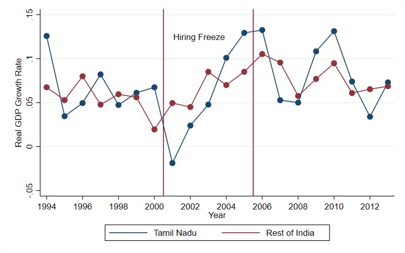
This paper also has implications for understanding optimal public sector hiring policy.
Motivated by a focus on improving service delivery, much of the existing literature has
focused on the eects of these policies on the set of people that are ultimately selected
(Dal Bó, Finan, and Rossi, 2013; Ashraf, Bandiera, and Jack, 2014; Ashraf, Bandiera,
Davenport, and Lee, 2020). By contrast, this paper redirects focus towards the vast
majority of candidates who apply but are not selected. In a context where this population
is largesuch as in Indiathe eect on this latter population appears to be large enough
that is worth considering this population explicitly when designing hiring policy.
More broadly, this paper helps us understand how workers respond to demand shocks
within highly desirable and salient sectors of the economy. When these shocks occur,
incumbent workers face a choice between doubling down, or cutting their losses. In the
United States, evidence from the manufacturing sector (a desirable and salient sector
for less-educated men) suggests that men tend to double down (Autor, Dorn, Hanson,
and Song, 2014). In this paper, I provide evidence from a dierent context for a similar
pattern of responses.
These results suggest that public sector hiring policy in India has the potential to
aect the entire labor market. This represents both an opportunity and a challenge:
hiring policy is a relatively unexplored policy lever for combating unemployment in this
context, but that also means that the chance that hiring policy decisions have unintended
consequences in the economy are also relatively high.
This paper proceeds as follows. Section 2 describes the competitive exam system in
India and provides details about the hiring freeze policy. Section 3 presents evidence on
the short-run labor supply impacts of the hiring freeze. Section 4 presents evidence on
the long-run impact of the hiring freeze on earnings. Section 5 discusses how the testing
environment in
uences candidates' response to the hiring freeze. Section 6 concludes.
6
2 Setting
2.1 The Competitive Examination System
In India, most administrative positionssuch as clerk, typist, and section o
cerare
9
lled through a system of competitive exams. All competitive exams include a multiple
choice test. For more skilled positions, the exam may also include an essay component
and/or an oral interview. The exam typically covers a wide range of academic subjects,
including history, geography, mathematics and logical reasoning, languages, and science.
The government conducts a single set of exams for batches of vacancies with similar job
descriptions and required quali
cations. After the results are tabulated, candidates then
10
choose their preferred posting according to their exam rank.
Government jobs advertised through competitive exams have eligibility requirements.
In Tamil Nadu, all posts require candidates to be at least 18 years of age and have a
minimum of a 10th standard education. Unlike other states, Tamil Nadu does not have
upper age limits for most applicants, and candidates can make an unlimited number
of attempts. In addition to 10th standard, some posts require require college degrees
and/or degrees in speci
c
elds. For recruitments completed between 1995 and 2010,
43% of posts and 25% of vacancies required a college degree.
These exams are heavily over-subscribed. Table 1 highlights a typical example from
Tamil Nadu for a recruitment advertised in 1999, a few years before the hiring freeze was
implemented. In this case, the Tamil Nadu government noti
ed 310 vacancies through
its Group 4 examination, which recruits for the most junior category of clerical workers.
It received 405,927 applications. Relative to the entire eligible population ages 18-40,
this corresponds to an application rate of about 5.6%. Because the application rate for
state-level government jobs is so high, it is plausible that changes in candidate behavior
could be re
ected in aggregate labor market outcomes.
9 The government also conducts exams for specialized positions, such as surgeons, scientists, statisti-
cians, and university lecturers.
10 In general, the exam process has enough integrity (especially in Tamil Nadu) that cheating is rare.
In cases where cheating is detected it is usually punished severely. For example, in Tamil Nadu 99
candidates were caught in a cheating scandal in January 2020 and were subsequently banned from
applying for government jobs for life (Rajan, 2020).
7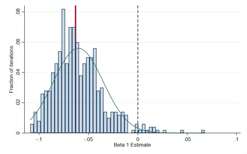
2.2 The Hiring Freeze
In November 2001, the Government of Tamil Nadu publicly announced that it would
suspend recruitment for non-essential" posts for an inde
nite period of time. Doctors,
police, and teachers were explicitly exempted from the hiring freeze. This meant that the
freeze applied mostly to administrative posts. In case a department wanted to make an
exception to the hiring freeze, it had to submit a proposal to a panel of senior bureaucrats
11 12
for approval. This policy was ultimately rescinded in July 2006.
According to the World Bank, the proximate cause of the hiring freeze appears to be
a
scal crisis, triggered by a set of pay raises that the Government implemented in the
late 1990s (Bank, 2004). Although other states experienced
scal crises around the same
13
time, to the best of my knowledge they did not implement a hiring freeze. I therefore
use the set of states excluding Tamil Nadu as a control group in the empirical analysis. I
test the sensitivity of the results to the choice of states included in the control group. To
the extent that other states also implemented hiring freezes at the same time, I expect
the estimated eects to be attenuated.
At the time of the hiring freeze, there were three government agencies in Tamil Nadu
responsible for recruitment: the Tamil Nadu Public Service Commission (which recruited
both administrative and medical posts); the Tamil Nadu Uniformed Services Board
(which recruited police); and the Tamil Nadu Teacher Recruitment Board (which re-
14
cruited primary and secondary teachers). Because the hiring freeze exempted teachers,
doctors, and police, the eect of hiring freeze thus fell entirely on recruitments conducted
by the Tamil Nadu Public Service Commission (TNPSC, hereafter). In Appendix Figure
A.2, I present evidence that recruitment in the exempt positions continued as usual.
Over the course of the
ve years of the hiring freeze, the Government made few
11 Speci
cally, proposals were vetted by a committee consisting of the Chief Secretary, the Finance
Secretary, and the Secretary (Personnel and Administrative Reforms).
12 The hiring freeze was announced in Tamil Nadu Government Order 212/2001. The freeze was lifted
in Government Order 91/2006.
13 To make this determination precisely, I would need to collect information from each of the state
governments. These requests for information are often denied on the grounds that they would require
too much time of the department's sta.
14 In 2012, the Tamil Nadu Government established the Tamil Nadu Medical Recruitment Board, which
took over responsibilities of recruiting medical sta from TNPSC.
8exceptions. There were only 15 exams conducted during the entire course of the hiring
freeze at TNPSC (of which 6 were for medical personnel), as opposed to an average of 28
per year when TNPSC was fully functional. As a result, as we see in Figure 1, the number
of available vacancies advertised by TNPSC fell by approximately 85% during the hiring
freeze. After the hiring freeze was lifted, the number of vacancies noti
ed returned to
roughly the same level it was at before the hiring freeze was announced.
The number of vacancies that were abolished due to the freeze was small relative to
the overall size of the labor force. A back-of-the-envelope calculation suggests that the
hiring freeze caused the most exposed cohorts of male college graduates to lose about
600 fewer vacancies over
ve years. Meanwhile, these same cohorts have a population
of about 100,000. So even if the hiring freeze caused a one-to-one loss in employment
(which is dubious, since family business is common), at most only about 0.6% the cohort's
employment should be aected. Even accounting for the large wage premium, the drop
in average earnings due to the aggregate demand shock is on the order of 0.4% of cohort-
average earnings. (See Appendix B for the details of these calculations). I therefore treat
the direct demand eect of the hiring freeze (i.e. the reduction in labor demand due to
less government hiring) as negligible, and ascribe any observable shifts in labor market
equilibrium to an endogenous supply response.
3 Short-Run Impacts of the Hiring Freeze
In this section, I assess whether and by how much the hiring freeze aected aggregate
labor market outcomes both during and in the years immediately following the hiring
freeze.
3.1 Changes in Labor Supply
3.1.1 Data
For this analysis, I use data from the National Sample Survey (NSS), a nationally repre-
sentative household survey conducted by the Government of India. I combine all rounds
9of the NSS conducted between 1994 and 2010 that included a module on employment.
This includes two rounds conducted before the hiring freeze; three rounds conducted dur-
15
ing the hiring freeze; and two rounds conducted after the end of the hiring freeze. By
stacking these individual rounds, I obtain a data set of repeated cross-sections.
My key outcome variable is employment status. I consider three categories: employed,
unemployed, and out of labor force. These variables are constructed using the NSS's Usual
Principal Status de
nition. Household members' Usual Principal Status is the activity
in which they spent the majority of their time over the year prior to the date of the
survey. In accordance with the NSS de
nition, I consider individuals to be employed if
their principal status included any form of own-account work, salaried work, or casual
labor. Individuals are marked as unemployed if they were available" for work but not
16
working. Relevant to this setting, individuals who are enrolled in school are considered
unemployed if they would consider leaving in order to take up an available job opportunity
(NSS Handbook). This means that individuals who continue to collect degrees while they
prepare for government examsas documented in Jerey (2010)would be marked as
unemployed. Being out of the labor force is the residual category among those who are
neither employed nor unemployed.
Unless otherwise noted, I adjust all estimates according to the sampling weights pro-
vided with the data. I normalize weights so that observations have equal weight across
17
rounds relative to each other.
3.1.2 Empirical Strategy
The key empirical challenge is to estimate how labor market outcomes would evolve in
Tamil Nadu in the absence of the hiring freeze. To construct this counterfactual, I use
a dierence-in-dierences (DD) design that compares Tamil Nadu with the rest of India,
15 Speci
cally, I use data from the 50th, 55th, 60th, 61st, 62nd, 64th, and 66th rounds. These surveys
were conducted during the following months, respectively: July 1993 - June 1994; July 1999 - June 2000;
January 2004 - June 2004; July 2004 - June 2005; July 2005 - June 2006; July 2007 - June 2008; and
July 2009 - June 2010. For simplicity, I refer to each round by the year in which it was completed.
16 Note that this de
nition does not include explicit criteria for active search.
17 That is: if w are NSS-provided weights for individual i in round r , and there are Nr observations
ir P
in round r, then the weights I use are: Nr ∗ wir r wir .
1018
and compares more aected cohorts with less aected cohorts.
Who is likely to be aected by the hiring freeze? The hiring freeze policy will
likely only aect a speci
c segment of Tamil Nadu's labor market. In general, Indian
states require that candidates who appear for competitive examinations have at least
a 10th standard education. In the year 2000, the year before the hiring freeze was
rst implemented, this requirement excluded about 70% of the population between the
ages of 18 to 40 in Tamil Nadu. Moreover, as we will see, application rates are very
heterogeneous within the eligible population. For these reasons, even though the total
number of applicants is large, the share of the overall population of Tamil Nadu that
would have been actively making application decisions during the hiring freeze is likely to
be relatively small. The NSS unfortunately does not provide me with enough statistical
power to measure the impact at an aggregate level. I therefore need to zoom in on the
segment of the population that is most likely to consider applying during the hiring freeze.
To estimate how application rates vary across demographic groups, I use administra-
tive data from the Tamil Nadu Public Service Commission for exams conducted between
2012 and 2014, and Census data from 2011. I estimate the application rate by dividing
counts of the average number of applications received by age by the population estimate
from the Census. The results of this calculation are presented in Figure 2. Note that
application rates vary widely by age and education. Application rates are highest among
college graduates around age 21, which is the year right after a typical student completes
19
an undergraduate degree.
Based on the observed variation in application rates, we should expect the largest
eect for cohorts that turned 21 during the hiring freeze. That is because this group was
most likely to make application decisions under usual conditions. This is my primary
treatment" group of interest. It is possible that cohorts that were older than 21 at
18 Throughout the analysis, I include observations from Puducherry in Tamil Nadu. Puducherry is a
small federally-administrated enclave entirely surrounded by Tamil Nadu, which shares the same language
as Tamil Nadu, and which does not have a Public Service Commission of its own. Residents of Puducherry
commonly apply for positions through the Tamil Nadu Public Service Commission.
19 A typical undergraduate degree starts at age 18 and lasts 3 years, which makes a typical fresh
graduate 21 years old.
11the time the hiring freeze was announced were aected. However, we would also expect
smaller eects sizes for this group relative to the group that graduated from college, since
many individuals from the former group would have exited exam preparation already.
Sample Restrictions. I restrict the sample in three ways: 1) I restrict the sample to
men. This is because, as we will see in Section 3.1.3, college graduation rates for women
shift after the hiring freeze, which makes it di
cult to disentangle the impact of the
hiring freeze from violations of the parallel trends assumption. 2) I restrict the sample to
individuals between the ages of 21 to 27 at the time the survey was completed, thereby
20
focusing on the sample that is most likely to apply for government jobs. 3) I further
restrict the sample to cohorts who were between the ages of 17 to 30 in the year 2001. The
lower bound corresponds to the youngest individuals who are expected to have graduated
21
from college before the end of the hiring freeze.
Regression Speci
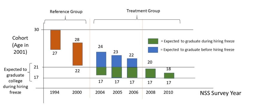
cation. Figure 3 summarizes the variation that I use. In each survey
year, I plot the cohorts that are included in the sample after implementing the restrictions
described in the preceding paragraph. I de
ne cohorts by their age in 2001, the year in
22
which the hiring freeze was announced. The comparison group includes all individuals
whose outcomes were measured before the start of the hiring freeze. The treatment group
includes all observations measured after the implementation of the hiring freeze belonging
to individuals who were expected to complete college before the end of the hiring freeze.
Throughout, I use age 21 as the expected age of college graduation. The treatment group
23
therefore includes seven cohorts, i.e. those between the ages of 17 to 24 in 2001. I divide
the treatment group into two groups: 1) those who are expected to have graduated from
college during the hiring freeze (i.e. age 17-21 in 2001); and 2) those who are expected to
20 For most rounds, the NSS was conducted over the course of a year. Assuming that birthdays are
roughly uniformly distributed, this means that about half of the sample will have aged another year
during the course of the survey. I can break the tie either way. I choose to break it by adding one to the
reported age for each individual in the sample.
21 There is no conceptual reason to include the upper bound. Its primary purpose is to exclude the
cohort that was age 31 in 2001, which is a severe outlier relative to all the other cohorts in the sample
(see Appendix Figure A.3). All the results hold if the cohorts older than 31 are included in the sample
as well.
22 Speci
cally, I compute [Age in 2001] = [Age] + (2001 − [NSS Round Completion Year]).
23 Given the sample restrictions and the timing of the NSS rounds, cohorts that were older than 24 of
age in 2001 were only surveyed before the hiring freeze was announced.
12have already graduated from college before the hiring freeze (i.e. age 22 to 24 in 2001).
My empirical strategy compares each of these groups to the comparison group in Tamil
Nadu and to its counterpart in the rest of India.
I implement these comparisons using the following regression speci
cation:
yi = β1 [T Ns(i) × Duringc(i) × F reezet(i) ] + β2 [T Ns(i) × Bef orec(i) × F reezet(i) ]
+ ζT Ns(i) + γc(i) + δF reezet(i) + Γ0 Xi + i (1)
Because the data consists of repeated cross-sections, each observation is a unique indi-
vidual. Cohorts c(i) are indexed according to their age in 2001. T Ns(i) is an indicator
for whether state s is Tamil Nadu. Duringc(i) and Bef orec(i) are indicators for whether
cohorts were expected to graduate either during or before the hiring freeze, respectively.
That is, Duringc(i) = 1 [17 ≤ c(i) ≤ 21] and Bef orec(i) = 1 [c(i) ≥ 22]. F reezet(i) is an
indicator for whether the individual was surveyed in a year t(i) after the hiring freeze
was implemented, i.e. F reezet(i) = 1 [t(i) ≥ 2001]. Finally, the vector Xi includes a set
of control variables, including: 1) dummy variables for the individual's age at the time
24
of the survey, interacted with T Ns(i) ; and 2) caste and religion dummies.
The primary coe
cients of interest are β1 and β2 . These parameters identify the
impact of the hiring freeze under a parallel trends assumption. Before the hiring freeze was
announced, Tamil Nadu and the rest of India had similar average rates of unemployment
and employment within the analysis sample (see Appendix Table A.3). The parallel
trends assumption requires that Tamil Nadu and the rest of India would continue to have
similar average outcomes in this sample across time if not for the hiring freeze.
To assess the validity of the parallel trends assumption it is standard practice to com-
pare trends before the implementation of the policy change. Unfortunately, the paucity
of data before the hiring freeze does not allow me to estimate pre-trends with enough
25
precision for this test to be informative. Instead, I implement an alternative over-
24 Both caste and religion are coded in groups of three. Caste is either ST, SC, or Other. Religion is
either Hindu, Muslim, or Other.
25 The sample sizes in state x cohort cells are often less than a hundred observations, especially for
older cohorts. See Appendix Table A.1.
13identi
cation test made available by the institutional context. Recall, individuals with
less than a 10th standard education are not eligible to apply for government jobs through
competitive exams (henceforth, I refer to this group as the ineligible sample). Therefore,
if the rest of India serves as a valid counterfactual, we should expect β1 = β2 = 0 when the
26
speci
cation in equation (1) is run on the ineligible sample. As with the pre-trends test,
this test is neither necessary nor su
cient for valid identi
cation in the college-educated
sample. However, because employment status tends to be correlated between the two
samples across years and states (see Appendix Figure A.4), it is plausible that shocks
to employment status are common across both samples, and hence this test should be
informative.
I also explicitly compare the coe
cients from the college sample with the coe
cients
from the ineligible sample using a triple dierence design. The full estimating equation
for this speci
cation is:
yi = Collegei × β1 [T Ns(i) ×Duringc(i) ×F reezet(i) ]+β2 [T Ns(i) ×Bef orec(i) ×F reezet(i) ]
0
+ γc(i),1 + δ1 F reezet(i) + Γ1 Xi + α
+ η1 [T Ns(i) × Duringc(i) × F reezet(i) ] + η2 [T Ns(i) × Bef orec(i) × F reezet(i) ]
0
+ γc(i),0 + δ0 F reezet(i) + Γ0 Xi + i (2)
27
Across both speci
cations, I cluster standard errors at the state-by-cohort level.
In doing so, I treat clustering as a design correction that accounts for the fact that
the treatment (i.e. exposure to the hiring freeze) varied across cohorts within Tamil
Nadu (Abadie, Athey, Imbens, and Wooldridge, 2017). Since cohorts are tracked across
multiple survey rounds, state-by-cohort clusters will also capture serial correlation in
28
error terms across years. Although the total number of clusters is large, traditional
26 This assumes that general equilibrium eects on the ineligible sample are negligible.
27 Several states split during this time period. I ignore these splits when assigning observations to
states, maintaining consistent state de
nitions across the 8 rounds of the NSS.
28 This approach is standard in the literature on the eects of graduating during a recession, which also
features shocks that vary in intensity across states and cohorts (Kahn, 2010; Oreopoulos, Von Wachter,
and Heisz, 2012; Schwandt and Von Wachter, 2019).
14clustered standard errors are still too small because the number of clusters corresponding
to the coe
cients of interest is also small (Donald and Lang, 2007; MacKinnon and
Webb, 2018). I therefore report con
dence intervals using the wild bootstrap procedure
outlined in Cameron, Gelbach, and Miller (2008). My own simulations indicate that these
29
con
dence intervals are likely to have nearly the correct coverage rate in this setting.
The validity of restricting to the analysis to a sample of college graduates depends
on whether college graduation rates moved in parallel in Tamil Nadu and the rest of
India. In Appendix Table A.4, I assess whether this is the case. For men, I observe no
statistically signi
cant changes in college completion after the hiring freeze. By contrast,
I see a large increase for women. It is unclear whether this shift re
ects a violation of
30
the parallel trends assumption or is an endogenous outcome of the hiring freeze. To
simplify the analysis, I therefore restrict the analysis to men.
3.1.3 Results
I begin by presenting the DD results for each treatment cohort using unadjusted cell
means. Although these estimates are imprecise, they allow us to more transparently assess
the underlying variation that informs the estimates from the parametric speci
cations.
To compute these estimates, I
rst compute unweighted averages of unemployment and
employment by state x cohort x year cells. For each treatment cohort, I compute a
simple DD estimate by subtracting the Tamil Nadu mean from the simple average of the
31
remaining states, and then comparing that dierence with the comparison group.
The results of this exercise are presented in Figure 4. Note that unemployment is
consistently higher (and employment consistently lower) among all cohorts that were
29 I construct the simulation as follows. For each of 500 iterations, I replace the dependent variable with
a set of random 0/1 draws that are i.i.d. across observations. I then tabulate the fraction of con
dence
intervals that include zero. The results are reported in Appendix Table A.2.
30 One reason why we might expect to see a parallel trends violation for women in particular is that this
period coincided with a large expansion in the set of available respectable work opportunities (especially
business process outsourcing work), which both aected educational attainment and were not uniformly
available across Indian states (Jensen, 2012).
31 In more precise terms: Let s index states, c t ∈ {0, 1} be an indicator for whether
index cohorts,
outcomes were measured after the hiring freeze, and
T Ns be an indicator for Tamil Nadu. Then for
each outcome y , I present estimates of:
E y | c, t = 1, T Ns = 1 − E y | t = 0, T Ns = 1 − E y | c, t =
1, T Ns = 0 − E y | t = 0, T Ns = 0 .
15expected to graduate from college during the hiring freeze. Meanwhile, among cohorts
that we expect to have already graduated, the estimates tend to hover around zero. The
consistency of the estimates across these two groups of cohorts suggets that it is unlikely
that estimates of β1 and β2 in equation (1) are driven by individual cohorts.
Panel A of Table 2 summarizes the estimates for equation (1). The coe
cients in
Column (1) indicate that, after the implementation of the hiring freeze, unemployment
among cohorts that were expected to graduate from college during the hiring freeze in-
creased by a statistically signi
cant 6.2 percentage points relative to the rest of India
(95% CI: 0.4 - 11.9 p.p.). This corresponds to a 6.2/20.7 = 30% increase in the likelihood
of unemployment. Meanwhile, we observe opposite-signed and statistically insigni
cant
eects on cohorts that were already expected to have graduated. These coe
cients cap-
ture the average shift in cohorts' labor market trajectory between the ages of 21 and 27.
The increase in unemployment could therefore re
ect both an intensive margin eect (i.e.
individuals spending more time in unemployment) and an extensive margin eect (i.e.
more people ever experiencing unemployment). In Columns (2) and (3) we see that the
increase in unemployment is almost entirely accounted for by a decline in employment.
Changes in labor force participation are negligible.
Panel B re-estimates equation (1) on the ineligible sample. For all three outcome
variables, the coe
cients are small and statistically insigni
cant. The null eect indicates
that, in the ineligible sample, men tended to follow the same early career trajectories
during the hiring freeze as their predecessors did prior to the hiring freeze. This provides
some reassurance that the parallel trends assumption is reasonable for men in this context.
Finally, in Panel C, I present estimates from the triple dierence speci
cation in
equation (2), which eectively estimates the dierence between the coe
cients of Panels
A and B. Since the coe
cients in Panel B are all close to zero, the point estimates in
Panel C are very similar to those in Panel A. The con
dence intervals are also nearly
identical.
163.1.4 Robustness
I probe the robustness of these results in three ways:
Choice of comparison group. I test whether the results in Table 2 are sensitive to the
choice of states to include in the comparison group. I try several variations. In Appendix
A.5 I use only the states that neighbor Tamil Nadu in the comparison group (namely
Karnataka, Kerala, and undivided Andhra Pradesh). In Appendix Table A.6, I only use
other large states, which I de
ne as those with at least 500 observations per state in
32
the sample of male college graduates. In both cases, the point estimates of β1 remain
very similar. As we would expect, the con
dence intervals are tighter when I use more
comparison states.
This lack of sensitivity to the choice of comparison states generalizes: I
nd that on
average I obtain the same estimate of β1 when I use a random subset of states in the
comparison group. That is, if I randomly sample 10 states from the set of comparison
states and re-estimate equation (1), the mean of this distribution nearly coincides with
the estimates of β1 reported in Table 2 (see Appendix Figure A.5). This is exactly what
we would expect if states experience common shocks across time and state-speci
c trends
are largely absent in this context.
Speci
cation. I probe robustness to dropping the caste and religion controls. In case
the types of individual completing college responded to the hiring freeze policy, these
controls may no longer be exogenous. These results are presented in Appendix Table
A.7. The estimates remain similar.
Alternative interpretations. So far, I have interpreted the estimates in Table 2 as
re
ecting shifts in labor supply. Here, I consider alternative interpretations of these
coe
cients.
In particular, one might be concerned about the direct eects of the conditions that
precipitated the hiring freeze in the
rst place. As discussed in Section 2, the Tamil Nadu
32 The states included in this sample are: undivided Andhra Pradesh, Bihar, Gujarat, Karnataka,
Kerala, undivided Madhya Pradesh, Maharashtra, Odisha, Punjab, Rajasthan, Uttar Pradesh (including
Uttarakhand), and West Bengal.
17government appears to have implemented the hiring freeze because it faced a
scal crisis.
In 2001, the same year as the implementation of the hiring freeze, Tamil Nadu experienced
a drop in GDP growth relative to the rest of the country (see Appendix Figure A.6). This
fact raises the possibility that the increase in unemployment is a result of the more well-
understood cost of graduating during a recession (Kahn, 2010; Oreopoulos et al., 2012;
Schwandt and Von Wachter, 2019). Furthermore, the labor market may be aected by
contemporaneous changes in service delivery or budget re-allocations.
The triple dierence speci
cation addresses these concerns to some extent: in general,
it is hard to conceive of a mechanism in which macroeconomic shocks only aect the co-
horts of college graduates most likely to apply for government jobs during the hiring freeze.
Still, it is possible that demand shocks for less educated individuals are not re
ected in
employment status, since their labor supply tends to be less elastic (Jayachandran, 2006).
To aid in distinguishing between demand- and supply-based interpretations of the
data, I study the impacts on earnings. Consider a simple supply and demand model of
the aggregate labor market, in which both curves have
nite elasticity. If the increase
in unemployment re
ects a reduction an aggregate labor supply, then we would expect
to observe an increase in average wages among the remaining participants in the labor
market. Conversely, if the increase in unemployment re
ects a drop in aggregate labor
demand, then see a decrease in wages.
To assess how wages responded to the hiring freeze, I use earnings data in the NSS.
Household members report the number of days employed in the week prior to the survey,
and their earnings in each day. I compute average wages by dividing weekly earnings
by the number of days worked in the week. I use the same speci
cation from the main
analysis (i.e. equation (1)), with the sample restricted to male college graduates who
reported any days of employment. Appendix Table A.8 summarizes these results. Mem-
bers of the cohorts age 17 to 21 in 2001 who chose to stay in the labor market had higher
earnings. This evidence, combined with the evidence on employment status, is consistent
with aggregate labor supply falling after the implementation of the hiring freeze.
183.2 Linking Unemployment to Exam Preparation
After the implementation of the hiring freeze, the cohorts that were most likely to be
aected spent more time unemployed. Why is this the case? In this section, I present
evidence that the most likely account is that they spent more time preparing full-time for
the exam. Unfortunately, in India there are no existing datasets that directly measure
exam preparation during this time period. However, if exam preparation did increase,
33
then we should observe an increase in the application rate during the hiring freeze.
Recall that not all recruitments were frozen during the hiring freeze. I can therefore test
whether recruitments conducted during the hiring freeze received more or less applications
than similar recruitments conducted before the hiring freeze.
3.2.1 Data
I digitized all the annual reports of the Tamil Nadu Public Service Commission that were
published between 1995 and 2010. These reports provide statistics for all recruitments
completed during the report year.
34
In the report, vacancies are classi
ed into state" and subordinate" positions. The
former include the highest level positions for which TNPSC conducts examinations. It
turns out that the only state-level recruitments conducted by TNPSC during the hiring
freeze were for specialized legal and medical positions (such as judge, surgeon, and vet-
erinarian), which were exempt under the hiring freeze (and thus these applicants should
be unaected). Therefore I focus the analysis on the sample of subordinate positions,
which re
ects 57% of posts and 75% of vacancies in this period.
3.2.2 Empirical Strategy
I compare recruitments conducted during the hiring freeze against those with similar
number of vacancies before the hiring freeze. The regression I estimate takes the following
33 Of course, it is possible that candidates appear for the exam without preparing. But, as we will see,
the fact that tougher exams receive fewer applications suggests that candidates tend to consider their
preparedness when deciding whether to apply.
34 On average, it takes 475 days between the date of last application and the date when the result is
announced. The maximum observed in the sample is 2998 days.
19form:
log yi = α + β1 f reezet(i) + β2 af tert(i) + γ log(vacancies)i + i (3)
where i indexes recruitments, and t(i) measures the year in which recruitment i was
noti
ed. The outcome of interest is application intensity, for which I observe two distinct
measures: 1) the number of applications received; and 2) the number of candidates who
appeared for the exam. The variable f reezet(i) is a dummy for whether the last date
to apply occurred while the hiring freeze was still in eect, and af tert(i) is a dummy
for whether the last date to apply occurred after the freeze was lifted. The variable
vacanciesi tracks the number of vacancies advertised in the recruitment. Recruitments
with fewer vacancies are typically those for more senior positions, which involve more
di
cult exams. Controlling for the number of advertised vacancies therefore proxies for
a range of dierent features of the advertised position.
The coe
cients β1 and β2 identify the impact of the hiring freeze under the assumption
that recruitments conducted before the hiring freeze are valid counterfactuals. To assess
the validity of this assumption, I explicitly check for trends by estimating the following
speci
cation:
log yi = αt(i) + γ log(vacancies)i + i (4)
The parameter of interest in this speci
cation is αt(i) . In the absence of meaningful pre-
trends, we should expect to see roughly constant values of of αt(i) before the hiring freeze,
and a sharp change in αt(i) during the hiring freeze.
3.2.3 Results
Figure 5a provides an approximate visual illustration of the regression in equation (3),
using applications received as an outcome variable. There were four recruitments con-
ducted during the hiring freeze. Those recruitments are labeled with the year in which the
recruitment was conducted. Relative to the number of advertised vacancies, the number
of applications received is much higher than usual. Table 3 summarizes estimates of the
magnitude of this dierence. The estimates indicate that applications increased by 301
20log points during the hiring freeze; that is equivalent to a 20-fold increase in the usual
application rate. The eect on the number of candidates that actually appeared for the
exam is even larger.
The increase in the application rate during the hiring freeze is not part of a long-
run trend. After the hiring freeze, the vacancy-application curve falls, but it does not
entirely return to the same level it was at before the hiring freeze. The point estimate
(β2 ) suggests that the number of candidates appearing for exams is still 173 log points
higher than the period before the hiring freeze. Still, this is meaningfully smaller than
the application level observed during the hiring freeze: a test of the equality of the β1
and β2 coe
cients rejects at the 1% level.
In Figure 5b, I plot year-by-year estimates of the change in the hiring freeze using
equation (4), which con
rms that the increase in the application rate during the hiring
freeze is not continuous with pre-trends.
4 Long-run Eects of the Hiring Freeze
In this section, I assess whether the hiring freeze had an impact on the earnings of cohorts
between 2014-2019, about a decade after the end of the hiring freeze.
4.1 Data
I use the Centre for Monitoring the Indian Economy's Consumer Pyramids Household
Survey (CMIE-CPHS). This survey follows a nationally-representative panel of approxi-
mately 160,000 households every four months, starting in January 2014. I use all waves
of data collected between January 2014 and December 2019.
In each wave, households report earnings for the previous four months.
35
My primary
outcome is labor market earnings, which includes, wages, overtime, bonuses, and income
36
from self-employment. The CMIE-CPHS reports nominal income
gures. I de
ate all
35 In the
rst wave (January to April 2014), respondents reported income for months that extended
into 2013. I drop observations that re
ect income from 2013.
36 The CMIE-CPHS documentation provides the following details on how this variable is constructed:
This is the income earned by each working member of the household in the form of wages.
21reported income values to their 2014 values using annual in
ation rates reported by the
World Bank.
37
As in Section 3, I identify cohorts by their age in 2001. I correct for measurement
error in the observed age using an imputation procedure detailed in Appendix C. I weight
all estimates using the sampling weights provided by CMIE.
4.2 Empirical Strategy
I adapt the cohort-based approach from Section 3 to study the impact on long run
outcomes. As in Section 3, I restrict the main analysis to male college graduates between
38
the ages of 17 to 30 in 2001. The main dierence is that I do not observe outcomes
measured before the hiring freeze. To accommodate, I will treat the cohorts age 27 to 30
in 2001 as the comparison group, assuming they are relatively unaected by the hiring
freeze. This is consistent with the evidence from Section 3 that older cohorts appear to
be unaected by the hiring freeze.
39
I estimate the following dierence-in-dierences speci
cation:
yit = β1 T Ns(it) × 1(17 ≤ cit ≤ 21) + β2 T Ns(it) × 1(22 ≤ cit ≤ 26)
+ ζT Ns(it) + γc(it) + αt + it (5)
This is the salary earned at the end of a month by the salaried people in India. If a
businessman takes a salary from the business, it is included here as wages. A salaried
person may earn a salary from his employers and may also work as a home-based worker
(for example, by giving tuitions). In such cases, the income earned from home-based work
is also added into wages. Wages can be paid at the end of a month, a week, a fortnight
or any other frequency. All of these are added into a monthly salary appropriately during
the capture of data. Wages includes over-time payments received. Wages also includes
bribes. If an employee is given a part of his/her income in the form of food or other goods,
the value of these is included in wages with a corresponding entry in the expenses of the
respective item head. If rent expenses are reimbursed by the employer, then it is included
in wages. A corresponding entry in expenses is be made only if such an expense is made.
37 Speci
cally, I compute [Age in 2001] = f loor([Age]−[Months between Survey Date and Jan 2001]/12).
38 Education is measured independently in each wave of the survey. Due to measurement error, the
measured education of individuals sometimes
uctuates. I assign individuals the maximum modal ob-
served education level.
39 Compared to equation (1), this speci
cation drops the age-speci
c dummies. That is because these
coe
cients would largely be collinear with the cohort eects, both because the CMIE-CPHS is a panel
and because there are no outcomes measured before the implementation of the hiring freeze.
22where yit is the outcome for individual i measured in month t. Note that while all the
variation in exposure to the hiring freeze is across individuals, the panel structure allows
us to measure individual outcomes more precisely. Cohorts are indexed according to their
age in 2001. The group of cohorts 1(17 ≤ ci ≤ 21) is intended to capture individuals
expected to graduate from college during the hiring freeze; the group 1(22 ≤ ci ≤ 26)
captures the individuals expected to graduate from college before the hiring freeze.
To assess the parallel trends assumption, I run the same speci
cation on the ineligible
sample, i.e. men with less than a 10th standard education. I also use this sample as part
of a triple dierence speci
cation that compares the dierence-in-dierences coe
cients
between the college and ineligible samples:
yit = Collegei × β1 T Ns(it) × 1(17 ≤ cit ≤ 21) + β2 T Ns(it) × 1(22 ≤ cit ≤ 26)
+ ζ1 T Ns(it) + γc(it),1 + αt,1
+ η1 T Ns(it) × 1(17 ≤ cit ≤ 21) + η2 T Ns(it) × 1(22 ≤ cit ≤ 26)
+ ζ0 T Ns(it) + γc(it),0 + αt,0 + it (6)
As before, for both speci
cations I cluster errors at the state x cohort level and report
95% con
dence intervals using the wild bootstrap.
4.3 Results
The same cohorts of men who spend more time in unemployment in the short run appear
to have lower labor market earnings in the long run. This result is summarized in Table
4. I am unable to detect eects on average earnings with any precision (Column (1)).
However, if I
nd suggestive evidence that aected men are less likely to appear in the
top of the earnings distribution. I
nd suggestive evidence that men who were 17 to 21 in
2001 are 6 percentage points more likely to earn less than Rs. 20,000 per month in 2014
INR (95% CI: -0.004 - 0.129). Note that Rs. 20,000 corresponds to the 75th percentile
of the earnings distribution in the rest of India for this cohort.
23Reassuringly, we do not see any of these same impacts for the ineligible sample (see
Panel B), or for cohorts who were already expected to have graduated from college before
the hiring freeze. The triple dierence estimates suggest that the eects on the college
sample are not driven by common shocks.
Taken seriously, the estimates in Column (2) imply a large drop in earnings. Recall,
the evidence in Section 3 suggests that about 6% of the population that graduated during
the hiring freeze spent an average of an extra year in unemployment. Assuming no
impact on the remaining population, these estimates imply that a single additional year
of studying caused all individuals studying for the exam to drop below the Rs. 20K
threshold. It is unlikely that we can account for this eect just based on the returns
to labor market experience, when Mincer regressions suggest that those returns are on
the order of 3% per year. One possible explanation is that aected men remain less
attached to the workforce and more reliant on family for
nancial support. Jerey (2010)
documents how men who prepare for government jobs tend to delay household formation,
which could increase
nancial dependence in the long-run. The evidence in Columns (3)
and (4) hints at that story: Although there is no indication of a shift in household
income (Column (4)), aected mens' earnings are a smaller share of total household
income (Column (3)). Further work is needed to assess this hypothesis more robustly.
5 Mechanisms
The results so far suggest that college graduates increased the amount of time they spent
preparing for the exam in response to the hiring freeze. There are two aspects of this
response that are puzzling.
First, why would candidates be willing to study longer because of a hiring freeze? As
we will see in this section, during normal testing years, almost all candidates in Tamil
Nadu drop out voluntarily. This suggests that time spent preparing for the exam is costly,
and that these costs bind. For some reason, the hiring freeze made candidates more willing
to incur the costs associated with additional exam preparation. What factors explain why
24You can also read