Showcasing Relationships between Neighborhood Design and Wellbeing Toronto Indicators - MDPI
←
→
Page content transcription
If your browser does not render page correctly, please read the page content below
sustainability

Article
Showcasing Relationships between Neighborhood
Design and Wellbeing Toronto Indicators
Richard R. Shaker 1,2,3,4, * , Joseph Aversa 1,3 , Victoria Papp 2 , Bryant M. Serre 1 and
Brian R. Mackay 2,3
 1    Department of Geography & Environmental Studies, Ryerson University, Toronto, ON M5B 2K3, Canada;
      javersa@ryerson.ca (J.A.); bryant.serre@ryerson.ca (B.M.S.)
 2    Graduate Programs in Environmental Applied Science & Management, Ryerson University, Toronto,
      ON M5B 2K3, Canada; victoria.papp@ryerson.ca (V.P.); brian.mackay@ryerson.ca (B.R.M.)
 3    Graduate Program in Spatial Analysis, Ryerson University, Toronto, ON M5B 2K3, Canada
 4    GeoEco Design, Syracuse, NY 13210, USA
 *    Correspondence: rshaker@ryerson.ca; Tel.: +1-416-979-5000

 Received: 28 December 2019; Accepted: 28 January 2020; Published: 30 January 2020

 Abstract: Cities are the keystone landscape features for achieving sustainability locally, regionally,
 and globally. With the increasing impacts of urban expansion eminent, policymakers have encouraged
 researchers to advance or invent methods for managing coupled human–environmental systems
 associated with local and regional sustainable development planning. Although progress has been
 made, there remains no universal instrument for attaining sustainability on neither regional nor local
 planning scales. Previous sustainable urbanization studies have revealed that landscape configuration
 metrics can supplement other measures of urban well-being, yet few have been included in public data
 dashboards or contrasted against local well-being indicators. To advance this sector of sustainable
 development planning, this study had three main intentions: (1) to produce a foundational suite of
 landscape ecology metrics from the 2007 land cover dataset for the City of Toronto; (2) to visualize and
 interpret spatial patterns of neighborhood streetscape patch cohesion index (COHESION), Shannon’s
 diversity index (SHDI), and four Wellbeing Toronto indicators across the 140 Toronto neighborhoods;
 (3) to quantitatively assess the global collinearity and local explanatory power of the well-being and
 landscape measures showcased in this study. One-hundred-and-thirty landscape ecology metrics
 were computed: 18 class configuration metrics across seven land cover categories and four landscape
 diversity metrics. Anselin Moran’s I-test was used to illustrate significant spatial patterns of well-being
 and landscape indicators; Pearson’s correlation and conditional autoregressive (CAR) statistics were
 used to evaluate relationships between them. Spatial “hot-spots” and/or “cold-spots” were found
 in all streetscape variables. Among other interesting results, Walk Score® was negatively related to
 both tree canopy and grass/shrub connectedness, signifying its lack of consideration for the quality
 of ecosystem services and environmental public health—and subsequently happiness—during its
 proximity assessment of socioeconomic amenities. In sum, landscape ecology metrics can provide
 cost-effective ecological integrity addendum to existing and future urban resilience, sustainable
 development, and well-being monitoring programs.

 Keywords: crime; data dashboard; landscape indicators; premature mortality; spatial autoregressive
 modeling; streetscapes; sustainable urbanization; Toronto; urban design; urban landscape; urban
 planning; walk score

1. Introduction
    Cities are the keystone landscape features for achieving sustainability locally, regionally, and
globally. In 2017, the United Nations predicted that the global population will grow to 9.7 billion

Sustainability 2020, 12, 997; doi:10.3390/su12030997                      www.mdpi.com/journal/sustainability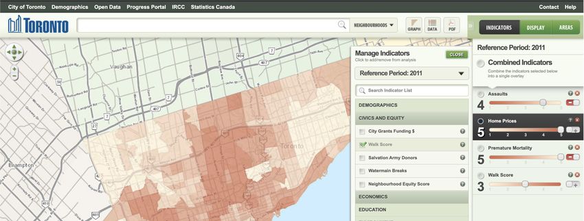
Sustainability 2020, 12, 997                                                                             2 of 24

inhabitants by 2050, and 11 billion inhabitants by 2100; however, it will be cities that absorb a majority
of the foreseen population growth in the developed and developing world [1]. As of 2008, homo
sapiens became more of an urban species rather than rural [2], and now there are 28 megacities
(population >10 million) and several nations with 100% urban population [3]. In a shocking prophecy
by Michael Batty [4], the global population is predicted to be 70% urban in 2050 and 100% urban
in 2092. Although cities have been recognized as leaders in socioeconomic well-being, catalysts for
educational and technological growth, and centers for historic preservation, culture and the arts [5–7],
their connected structure has been found to simultaneously degrade Earth’s life-supporting systems [8].
Urbanization, directly and indirectly, metabolizes Earth’s healthy environmental resources and disturbs
life-supporting ecosystem services great distances from urban centers [9–16]. Consequently, land cover
change associated with population growth, rural to urban migration, a desire for greater material
well-being, and poor waste management are having the greatest impacts on Earth’s life-supporting
biogeochemical systems and thus its planetary boundaries [10,15,17–25].
      With the increasing impacts of urban expansion eminent [4,11,13,26], policymakers have
encouraged researchers to advance or invent methods for managing coupled human–environmental
systems associated with local and regional sustainable development planning [27]. Furthermore, for
roughly two decades now, the planning community has seen a need for sustainable development
initiatives that go beyond lip-service and put concepts into action [28–30]. Despite uncertainty about
operationalization, the field of planning acknowledges that sustainable development is an influential
concept and should shape future methodology and practice [31–33]. That said, although effort and
progress have been made, there remains no universal instrument for attaining sustainability on neither
regional nor local planning scales [34]. As suggested by Jianguo Wu [5–7], landscape ecology is
likely the most relevant place-based and solution-driven discipline for moving humanity towards
sustainability across space and time. Landscape ecology emphases two main principles of landscape:
(i) patterns, or the physical configuration of its elements (i.e., urban land connectivity); and (ii) processes,
or its biogeophysical functions (i.e., disrupted hydrological cycle) that modify or result from its spatial
structure [35]. Despite numerous environmental management, conservation, restoration, urban and
regional planning projects incorporating landscape ecology tools and methods, work remains for
landscape sustainability science to move theory into everyday planning practice [36,37].
      Indicators and their combined forms, indices, are essential tools for calibrating landscape structure
during sustainable urbanization, urban resilience, environmental planning and management projects.
At local and regional scales, indicator-based assessment of landscape function is a fundamental
approach for evaluating relationships during sustainable landscape planning [38,39]. An evaluation
metric takes the form of a rapidly employable single-number characterization of a location at a given
time [40], which have been embraced widely for urban design, ecosystem management, natural resource
conservation, sustainable urbanization, environmental and regional planning purposes [8,14,23,41].
Spatial planning investigations of human-dominated landscapes have been further understood using
analytical tools for quantifying landscape structure (e.g., FRAGSTATS) and spatial analysis software
(e.g., SAM) [14,41]. That said, few urban ecology studies serve as examples of how landscape patterns
respond to indicators of urban well-being and resilience at local and regional scales. Lastly, because
spatial autocorrelation [42] is inherently present during urban well-being assessments, appropriate
inferential statistical methods (i.e., spatial autoregression) must be considered to correct for its
accompanying errors.
      Cultivating knowledge on how to optimize the urban mosaic is mandatory for creating urban
resilience and sustainable cities. Urban patterns and processes offer both problems and solutions for
sustainable development; however, they allow an opportunity to test questions related to what is the
‘optimal’ urban form [26]. Previous sustainable urbanization studies have revealed that landscape
configuration metrics can supplement other measures of urban well-being (i.e., [43]), yet few have
been included in public data dashboards or contrasted against local well-being indicators. To advance
this sector of sustainable development planning, this study had three main intentions: (1) to produce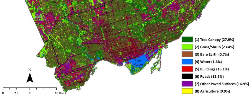
Sustainability 2020, 12, 997                                                                          3 of 24

a foundational suite of landscape ecology metrics from the 2007 land cover dataset for the City of
Toronto; (2) to visualize and interpret spatial patterns of neighborhood streetscape patch cohesion index
(COHESION), Shannon’s diversity index (SHDI), and four Wellbeing Toronto indicators across the
140 Toronto neighborhoods; and (3) quantitatively assess global collinearity and local explanatory
power of the well-being and landscape measures showcased in this study. A goal of this study
was to justify adding landscape ecology metrics into urban resilience, sustainable development, and
well-being monitoring programs. This paper was also created to deliver sustainability scientists, spatial
analysts, urban planners and designers an applied example for systematically assessing, describing,
and monitoring sustainable landscape function across space.

2. Study Area
      This research incorporated all 140 neighborhoods as individual streetscapes for the City of Toronto,
located in the province of Ontario, Canada (Figure 1). The City is central to Southern Ontario’s
megalopolis, dubbed the “Golden Horseshoe,” which is a band of ever-increasing population growth
and subsequent urbanization wrapping the Provincial coastline of Lake Ontario [44–48]. As a leading
port city on the Laurentian Great Lakes of North America, with access to the Atlantic Ocean by way
of the Saint Lawrence Seaway, and land connections via major railways, Toronto was historically a
place of mercantile prosperity and has grown into Canada’s most populated, culturally diverse, and
economically important city [49–52]. The 140 distinct neighborhoods have unique identities stemming
from different demography and responding built and natural forms [52–55]. With an area of 641km2 ,
a population of 2.95 million in July 2018, and a density of 4457 persons/km2 , the City of Toronto
shares similarities with other North American metropolises as Montreal, Chicago, Philadelphia, and
Washington at 4916, 4594, 4512, and 4301persons/km2 , respectively [56–58]. However, Toronto is
differentiated from other North American cities because it is seen as one of the fastest-growing urban
centers, if not the fastest [51,59,60]. Increasing urbanizing pressures, the Greater Toronto Area (GTA) is
encircled by 800,000 hectares of protected land, known as the Greenbelt, which includes such natural
amenities as the Niagara Escarpment, Oak Ridges Moraine, and protected countryside [61].
      The City of Toronto has been dubbed the most resilient city in the world [62], yet it is projected that
its population growth will require innovative and adaptable urban sustainable development initiatives.
Toronto’s good reputation as a livable city and prosperous urban region is linked to its economic and
social welfare and the goods and services that are provided to its citizens [63]. In example, an effort
has been made to preserve its natural spaces and support Torontonians’ connection to nature; the
greenspace ravine systems and parks comprise nearly 17% of the city’s net area [64–67]. However,
over the last few decades Canadian societies, specifically in Toronto, have been changing. Economic,
social, and environmental trends are posing significant challenges to securing improved well-being
and promoting equitable and sustainable order within Canadian communities [68,69]. Toronto is
beginning to show signs of distress (i.e., congested streets) and imbalance in areas such as housing and
income security; without immediate action, the trends unfolding are likely to lead to a further decline
in the City’s well-being [51]. There is a need to evaluate current conditions and to determine the future
path towards sustainability for Toronto’s 140 neighborhoods using measurements of well-being. With
its interesting human and physical geography, growing population, and confined limits to growth,
Toronto’s complex coupled urban landscapes are fashionable for examining how patterns of streetscapes
relate to urban well-being.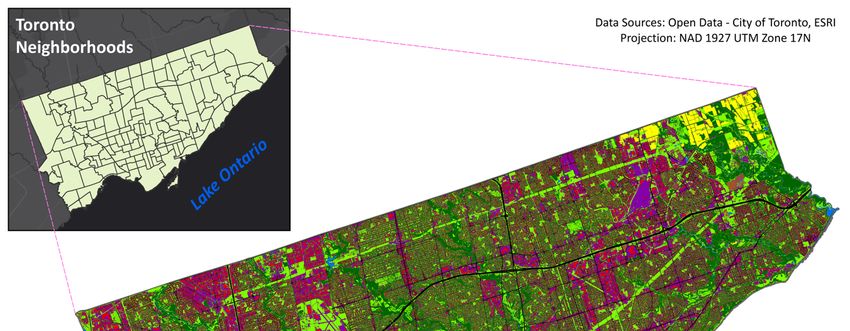
metropolises as Montreal, Chicago, Philadelphia, and Washington at 4916, 4594, 4512, and
4301persons/km2, respectively [56–58]. However, Toronto is differentiated from other North
American cities because it is seen as one of the fastest‐growing urban centers, if not the fastest
[51,59,60]. Increasing urbanizing pressures, the Greater Toronto Area (GTA) is encircled by 800,000
Sustainability
hectares of2020, 12, 997 land, known as the Greenbelt, which includes such natural amenities as
               protected                                                                      4 ofthe
                                                                                                   24
Niagara Escarpment, Oak Ridges Moraine, and protected countryside [61].

     Figure 1. Study area map of the 140 neighborhood-landscapes (streetscapes) in Toronto, Canada (43◦ 39’N,
     79◦ 20’W). Source neighborhood Geographic Information System (GIS) data freely downloadable from
     the City of Toronto’s Open Data Portal website (http://open.toronto.ca/).

3. Materials and Methods

3.1. Wellbeing Toronto Indicators
      Indicators and their composite versions indices are being used across spatial scales to address
multiple planning and policy-making objectives, and are considered indispensable in the science and
practice of sustainability [70–75]. These metrics are often quantitative expressions of spatial-temporal
sustainability, resilience, or well-being in context to a system’s current state. At the international level,
a call for these indicators happened at the Rio Earth Summit in 1992, which has resulted in a plethora of
public and private organizations responding at all scales of application [33,72,76,77]. From Chapter 8.6
of Agenda 21 [78] “Countries could develop systems for monitoring and evaluation of progress towards
achieving sustainable development by adopting indicators that measure changes across economic,
social and environmental dimensions” (66). Regarding unifying methods for assessing sustainable
urbanization, the International Organization for Standardization (ISO) is leading the way with ISO
37120:2018 [Sustainable cities and communities—Indicators for city services and quality of life] and
ISO 37122:2019 [Sustainable cities and communities—Indicators for smart cities] initiatives [79,80].
Although not free of charge, ISO has organized and standardized a set of indicators for city quality
of life, resilience, services and ‘smart cities’; furthermore, these standards act as proxies to help
cities support policy creation and priority planning initiatives. Despite the aforementioned efforts,
critical reviews of indicators and indices employed at the local level consider them ‘sub-optimal’ tools
for technical assessment, public participation, and use [70,73]. Specifically, when using indicators
and indices errors come from confusion or disagreement around variable selection, directionality,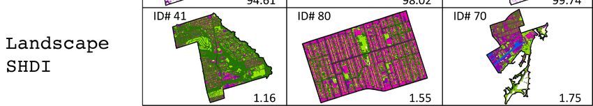
Sustainability 2020, 12, 997 5 of 24
normalization, weighting, and aggregation, as well as boundary delineation, stake-holder inclusion,
spatial analysis needs, and best practices [71,72,75,81–85].
Specific to Canada, in 2016 and reiterated in 2018, the federal government has shown a strong
commitment to developing technically sound evidence-based indicators for making progress toward
Sustainable Development Goals [86]. This, of course, builds on a long-standing history of indicator
creation and use in Canada from the internationally acclaimed Ecological Footprint [87] to the Canadian
Index of Well-being [68] to the Wellbeing Toronto discussed more herein. In response to the growing
need to measure well-being, the City of Toronto (the municipal government of Toronto) launched
“Wellbeing Toronto” in 2011, a web-based measurement and visualization data dashboard that helps
evaluate community
Sustainability well-being across a multitude of factors such as, crime, housing, and transportation
2020, 12, 997 5 of 25
(Figure 2). Wellbeing Toronto was developed to provide information to citizens and decision-makers
transportation
and to enable a(Figure
better 2). Wellbeing Toronto
understanding of howwas developed
their communities to provide information
function, based on to the
citizens and
metrics
decision‐makers
provided [88]. This andspatial
to enable a better understanding
decision-making tool uses of a how their online
modified communities function,
geographic based on
information
the metrics
system (GIS) to provided
visualize[88]. This
a suite spatial decision‐making
of well-being indicators across tool
theuses
City’sa 140
modified online geographic
neighborhoods. The free
informationallows
application system (GIS)
users to visualize
to select a suitevarious
and/or combine of well‐being indicators
indicators, acrossinstantaneously
which appear the City’s 140
neighborhoods.
on a map of Toronto The and
free produce
application allowsof
a variety users to select
graphs and/or all
and tables, combine various
of which indicators,
are free which
to download.
appear instantaneously on a map of Toronto and produce a variety of graphs and
Without going into detail about its unresolved flaws, Wellbeing Toronto’s shortcomings impacting this tables, all of which
are free
study to to:
relate download. Without
its inability going into
to normalize count detail
data about its unresolved
(i.e., assaults) by even flaws, Wellbeing
the most commonToronto’s
method
shortcomings impacting this study relate to: its inability to normalize count data (i.e.,
(i.e., population, area) circumventing the effects of different sized area units (i.e., Modifiable Areal Unit assaults) by
even the most common method (i.e., population, area) circumventing the effects
Problem; MAUP [89]); and its low representation of ecological integrity, environmental public health, of different sized
area unitsservices,
ecological (i.e., Modifiable Areal Unit Problem;
and biogeophysical indicators.MAUP [89]); and its low representation of ecological
integrity, environmental public health, ecological services, and biogeophysical indicators.
Figure2.2.Screenshot
Figure Screenshotofofthe
theCity
CityofofToronto’s
Toronto’smapping
mappingdata
datadashboard,
dashboard,Wellbeing
WellbeingToronto.
Toronto.Publicly
Publicly
accessibleat:
accessible at:http://map.toronto.ca/wellbeing/.
http://map.toronto.ca/wellbeing/.
Toaccomplish
To accomplishthis
thisstudy’s
study’smain
mainintentions
intentionsand
andsupplementary
supplementarygoals,
goals,four
fourofofthe
the2011
2011Wellbeing
Wellbeing
Torontoindicators
Toronto indicatorswere
wereselected
selectedfrom
fromthe thedata
datadashboard
dashboardforforcontrasting
contrastingagainst
againstthemselves
themselvesand and
landscapeecology
landscape ecology metrics.
metrics. Specifically,
Specifically, the urban
the four four well-being
urban well‐being metricstochosen
metrics chosen showcase to streetscape
showcase
streetscape relationships
relationships were:home
were: assaults, assaults, home
prices, prices, premature
premature mortality,mortality,
and Walkand WalkFrom
Score. Score.theFrom the
Safety
Safety domain,
domain, 2011 assaults
2011 assaults were sourced
were sourced from Toronto
from Toronto Police Service;
Police Service; there15,179
there were were 15,179
assaultsassaults
in totalin
total the
across across
City,the
withCity, with a of
a minimum minimum of nine,
nine, average average
of 108, of 108, of
and maximum and712maximum of 712 in one
in one neighborhood. To
neighborhood. To avoid spurious findings caused by MAUP, the 2011 assault counts
avoid spurious findings caused by MAUP, the 2011 assault counts were divided by their corresponding were divided
by their corresponding
neighborhood population.neighborhood
From the Housing population. From prices
domain, home the Housing domain,
were sourced fromhome prices were
Realosophy.com,
sourced from Realosophy.com, represents the average price (CAD) for residential real estate sold
during the 2011‐2012 timeframe. The average neighborhood home price minimum was $204,104, the
mean was $548,193, and the maximum was $1,849,084. From the Health domain, premature mortality
was sourced from Toronto Public Health from the 2006–2008 period and represents all‐cause
premature mortality per 100,000 population. Population data used here come from Statistics Canada,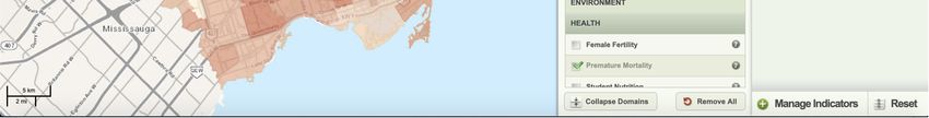
Sustainability 2020, 12, 997                                                                             6 of 24

represents the average price (CAD) for residential real estate sold during the 2011-2012 timeframe. The
average neighborhood home price minimum was $204,104, the mean was $548,193, and the maximum
was $1,849,084. From the Health domain, premature mortality was sourced from Toronto Public
Health from the 2006–2008 period and represents all-cause premature mortality per 100,000 population.
Population data used here come from Statistics Canada, 2006 Census of Canada. For clarification,
Canada’s premature mortality is a measure of unfulfilled life expectancy with an age expectation
set to 70; the premature mortality rate is the sum of potentially lost years of individuals per 100,000
people [90]. Descriptive statistics for premature mortality reflected 108 (min), 217 (mean), and 615
(max). Lastly, from the Civics and Equity domain, Walk Score was sourced from walkscore.com; Walk
Score is scaled from 0-100 based on walking routes and proximity to socioeconomic amenities such as
grocery stores, schools, parks, restaurants, and retail. With increased values representing improved
walkability, 2011 Walk Scores across the 140 neighborhoods had a minimum value of 42, average of 72,
and maximum of 99.

3.2. Streetscape Configuration and Diversity
      Neighborhood-landscapes (streetscapes) are inherently interconnected geophysical, biological,
and socioeconomic systems, and connect to human behavior through geographical identity. Because of
this, and the readily available well-being data from the Wellbeing Toronto data dashboard, this urban
spatial aggregation scale was deemed suitable for this study. Although there is no omnipresent rule for
“landscape scale,” or in this case streetscapes Richard T.T. Forman [91] suggested that a “landscape” is
“a kilometers-wide mosaic over which local ecosystems recur.” The area descriptive statistics across
the 140 Toronto neighborhoods are: 0.42 km2 (min), 4.59 km2 (mean), and 37.53 km2 (max). Within
each of the 140 neighborhood streetscapes, land cover class configuration and landscape diversity
metrics were calculated using fine spatial and categorical resolution land cover data created for the
City of Toronto in 2007 [92]. Produced from high-resolution QuickBird (Digital Globe) satellite imagery,
combined with planimetric data, this land cover raster layer has 0.6 m (1.9685 ft) pixels allowing for
single tree detection [93]. Although accuracy details for this data file could not be found, the same
research group and methods applied to New York City rendered an overall classification accuracy of
96% [14,94]. This high-resolution land cover data set was classified into eight land cover categories:
(1) tree canopy, (2) grass/shrub, (3) bare earth, (4) water, (5) buildings, (6) roads, (7) other paved surfaces,
and (8) agriculture (Figure 3). The 2007 land cover yielded the following compositions for the Toronto
categories: tree canopy (27.9%), grass/shrub (23.4%), other paved surfaces (16.9%), buildings (16.1%),
roads (12.5%), water (1.6%), agriculture (0.9%), bare earth (0.7%).
      Land cover configuration and landscape diversity metrics were computed using the freeware
FRAGSTATS (ver. 4.2; [95]), which processes numerical expressions that correspond to a landscape’s
land use and land cover patterns. Hundreds of metrics for quantifying landscape composition,
configuration, and diversity have been developed for use in a countless number of planning,
socioeconomic and environmental science research applications [16,91,96,97]. Based on literature
relevance and past experiences, for each of the 140 Toronto streetscapes, 130 landscape ecology metrics
were computed to serve as a foundational suite for the City of Toronto (Data S1): 18 class configuration
metrics across seven of the City’s eight land cover categories and four landscape diversity metrics.
Metrics for agriculture were not included due to very limited neighborhood representation. The 18 class
configuration metrics computed for each of the seven land cover types were: class area (CA), percentage
of landscape (PLAND), patch density (PD), largest patch index (LPI), landscape shape index (LSI), mean
patch area (AREA_MN), area-weighted mean patch area (AREA_AM), area-weighted mean shape
index (SHAPE_AM), area-weighted mean patch fractal dimension (FRAC_AM), perimeter-area fractal
dimension (PAFRAC), area-weighted core area distribution (CORE_AM), area-weighted core area index
(CAI_AM), area-weighted mean Euclidean nearest neighbor distance (ENN_AM), clumpiness index
(CLUMPY), percentage-of-like-adjacency (PLADJ), patch cohesion index (COHESION), landscape
division index (DIVISION), and effective mesh size (MESH). Additionally, the four landscape diversity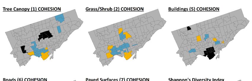
Globe) satellite imagery, combined with planimetric data, this land cover raster layer has 0.6 m
(1.9685 ft) pixels allowing for single tree detection [93]. Although accuracy details for this data file
could not be found, the same research group and methods applied to New York City rendered an
overall classification accuracy of 96% [14,94]. This high‐resolution land cover data set was classified
into  eight land
Sustainability 2020, cover
                     12, 997 categories: (1) tree canopy, (2) grass/shrub, (3) bare earth, (4) water, (5) buildings,
                                                                                                              7 of 24
(6) roads, (7) other paved surfaces, and (8) agriculture (Figure 3). The 2007 land cover yielded the
following compositions for the Toronto categories: tree canopy (27.9%), grass/shrub (23.4%), other
metrics   were: Patch
paved surfaces              richness
                      (16.9%),       density
                                 buildings     (PRD),roads
                                            (16.1%),  Relative  patchwater
                                                            (12.5%),  richness  (RPR),
                                                                            (1.6%),    Shannon’s
                                                                                    agriculture    diversity
                                                                                                (0.9%),   bareindex
                                                                                                               earth
(SHDI),
(0.7%).    and   Shannon’s      evenness  index   (SHEI).

     Figure 3. Map of 2007 land cover for Toronto, Canada. Source land cover data freely downloadable
     Figure 3. Map of 2007 land cover for Toronto, Canada. Source land cover data freely downloadable
     from the City of Toronto’s Open Data Portal website (http://open.toronto.ca/).
     from the City of Toronto’s Open Data Portal website (http://open.toronto.ca/).
     To accomplish this study’s intentions and goals, by showcasing how landscape ecology metrics
relateLand  coverwell-being,
       to urban   configurationfiveand landscape
                                    land          diversity
                                         cover (tree canopy,metrics were computed
                                                              grass/shrub, buildings, using
                                                                                      roads, the  freeware
                                                                                              other paved
FRAGSTATS      (ver. 4.2; [95]), which processes  numerical  expressions that correspond  to
surfaces) class COHESION measures and the landscape diversity metric SHDI were showcased in  a landscape’s
the forthcoming data analysis section (Figure 4). Specifically, COHESION at the class-level measures
the physical connectedness of the corresponding land cover type; its score ranges between 0 and 100
and increases as the patch type become more aggregated and physically connected [98]. Although
other relationships await to be explored within the plethora of landscape ecology metrics computed
herein, COHESION was chosen to showcase in this study due to its traction already gained in the
sustainable development and spatial planning communities. To that end, Meerow and Newell [43]
included forest cover COHESION as one of their model criteria to capture physical connectedness of
wildlife habitat across census tracts during their spatial planning effort to improve urban resilience in
Detroit. Precedingly, in a macroscale assessment of sustainable urbanization for Europe, Shaker [8]
used COHESION to compute the physical connectedness of CORINE urban morphological zones
for each country landscape. From that study, increased connectivity of urban cover COHESION
was simultaneously linked to improved human well-being while deteriorating ecosystem well-being.
SHDI [99], the most popular diversity index based on information theory and commonly used in
landscape studies [23], is a rather abstract mathematical model that is most useful when comparing
different landscapes or the same landscape over time [96]. The single number values of SHDI grow
without limits; SHDI increases as the quantity of land cover classes present increases and/or their
Sustainability 2020, 12, 997 8 of 24
proportions become more equal [96]. The premise behind showcasing relationships between SHDI
and well-being indicators was centered around the increasing importance of understanding how
landscape diversity of urban design relates to inhabitants’ living conditions. Accompanying maps
and statistical figures for the five class COHESION metrics and SHDI are provided in Appendix A
Sustainability
(Appendices 2020, 12, 997
A.1–A.3). 8 of 25
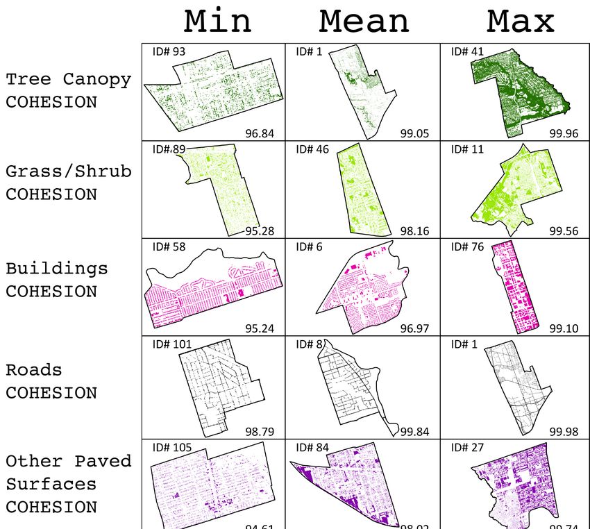
Figure
Figure 4. Streetscapesof
4. Streetscapes ofthe
thefive
five land
land cover
cover class
class COHESION
COHESION metrics metrics and
and one
one landscape
landscape diversity
diversity
SHDI metric
SHDI metric showcased
showcased in in this
this study.
study. Values
Valuesinin the
the lower‐right
lower-right corner
corner are
are raw
raw metric
metric scores
scores
corresponding to
corresponding to its
itsdescriptive
descriptive statistic. Upper-left
statistic. corner
Upper‐left labelslabels
corner matchmatch
the City of Toronto’s
the universal
City of Toronto’s
neighborhood
universal identification
neighborhood number enumerated
identification in public spatial
number enumerated and tabular
in public data.
spatial Cartographic
and note:
tabular data.
Neighborhood-landscapes are not equal geographic scale.
Cartographic note: Neighborhood‐landscapes are not equal geographic scale.
3.3. Data Analysis
3.3. Data Analysis
To accomplish the second and third intentions of this paper, and its complementary goals, a
To accomplish the second and third intentions of this paper, and its complementary goals, a
three-step analysis was created to visualize and showcase relationships between neighborhood
three‐step analysis was created to visualize and showcase relationships between neighborhood
COHESION, SHDI, and four Wellbeing Toronto indicators across the 140 Toronto streetscapes.
COHESION, SHDI, and four Wellbeing Toronto indicators across the 140 Toronto streetscapes.
Specifically,exploratory
Specifically, exploratoryspatial
spatialdata
data analysis
analysis (ESDA),
(ESDA), global
global and and
locallocal inferential
inferential statistical
statistical tests
tests were
were used and will be explained in detail here. Prior to employing the statistical tests, to
used and will be explained in detail here. Prior to employing the statistical tests, to meet parametricmeet
test requirement of Gaussian distributions, all variables evaluated in this study were appraised using
the Shapiro–Wilk test due to its power for determining normality for all types of distributions and
sample sizes [100]. In doing so, variables were determined if transformation was required, and which
mathematical function was most appropriate for reaching a Gaussian frequency. For variables with
straight values or counts, such as property values or number of assaults, log‐transformation wasSustainability 2020, 12, 997 9 of 24
parametric test requirement of Gaussian distributions, all variables evaluated in this study were
appraised using the Shapiro–Wilk test due to its power for determining normality for all types
of distributions and sample sizes [100]. In doing so, variables were determined if transformation
was required, and which mathematical function was most appropriate for reaching a Gaussian
frequency. For variables with straight values or counts, such as property values or number of assaults,
log-transformation was used. For ratio or percentage variables ranging from 0 to 1 or 0 to 100, such as
Walk Score, the empirical logit-transformation was used as it supersedes arcsine variants [101] and is
an improvement over simple logit [102]. The statistical software SPSS (ver. 25, [103]) was used during
this step of data preparation, and database used in the subsequent analysis provided here (Data S2).
First (1), to assess the level of spatial autocorrelation and to visualize local clustering an ESDA
was conducted at global and local levels. Spatial autocorrelation, the lack of univariate stationarity or
independence of an attribute over space, is the result of assessing the first law of geography [42]. Spatial
autocorrelation should be seen as both beneficial and problematic in urban resilience, sustainable
development, and well-being studies. Negatively, spatial autocorrelation violates the assumption of
independence required by traditional parametric tests (i.e., ordinary least squares regression) [104,105].
Positively, nonstationarity (spatial autocorrelation) can provide statistically significant meaning
to geographical patterns of sustainable development, and thus urban resilience and well-being
investigations; furthermore, ‘hotspots’ maps are often created to reflect these spatial relationships [106].
Although other procedures have been created to assess spatial non-stationarity, the original global
Moran’s I-test [107] was used to assess the level of spatial autocorrelation of the selected well-being
and landscape measures across the study area. Additionally, to illustrate the geographic clustering of
the six landscape ecology metrics and four well-being indicators, the local index of spatial association
(LISA) Anselin Moran’s I [108] was conducted. Using ESRI’s ArcMap (ver. 10.4; [109]) Incremental
Spatial Autocorrelation tool, a distance threshold of 3.5 km was established and used for both spatial
autocorrelation tests.
Secondly (2), a two-tailed Pearson’s Product–Moment Correlation test (r) was used to assess
relative statistical relationships between the five land cover class COHESION metrics, SHDI, and four
Wellbeing Toronto indicators (n = 140). Pearson’s correlation coefficients range from 1 to –1, with
values closer to 1 indicating stronger bivariate association. Pearson’s Product–Moment Correlation
test is one of the most common global (without considering geographic location and spatial influence)
parametric tests for understanding bivariate inferential relationships, and a P-value accompanies the
coefficient value signifying its statistical significance. The statistical software SPSS (ver. 25, [103]) was
used during this step of the analysis.
Third (3), bivariate local (considering geographic location and spatial influence) conditional
autoregressions (CAR) were conducted between- the five land cover class COHESION metrics and
SHDI- with the four chosen Wellbeing Toronto indicators (assaults, home prices, premature mortality,
and Walk Score). Since coupled human–environmental systems and data are impacted by a variety of
processes over space, local methods that address the shortcomings of spatial autocorrelation should
be used [105,110,111]. CAR corrects for spatial non-stationarity by calculating the spatial error terms
of the model and adds a distance-weighted function between adjacent response variable values
and the regression’s neighboring values for each explanatory variable [105,112,113]. Coefficient of
determination (R2 ) was used to compare and contrast relative explanatory power of the bivariate
regressions; standardized beta coefficient (β) was used to corroborate association strength and interpret
relationship directionality. CAR models used an estimated rho per regression and Alpha set to 1.0;
CAR model residuals were assessed ex post facto by global Moran’s I statistic to confirm model
independence. The freeware Spatial Analysis in Macroecology (SAM; ver. 4, [114]) was used during
this step of the analysis.Sustainability 2020, 12, 997 10 of 24
4. Results
4.1. Exploratory Spatial Pattern Analysis
Spatial autocorrelation test results differ from each other; however positive scores indicate
similar values are spatially clustered and negative scores indicate unlike values are systematically
separated [115]. For this study, Global Moran’s I-test divulged that all six landscape and four urban
well-being measures used in the analysis had less than 1% chance of occurring randomly across
space (Table 1). Across Toronto’s 140 neighborhoods, Anselin Moran’s-I [108] illustrated statistically
significant spatial “hot-spots” and/or “cold-spots” for all streetscape variables showcased. Discrete
categorical groupings of Local Anselin Moran’s-I indicate that a geographic feature has statistically
significant (0.05 level) clustering of neighboring features with similarly high (high-high; hot-spot) or
low (low-low; cold-spot) attribute values within a defined distance; outliers are recorded when a high
value is surrounded primarily by low values (high-low) or vise-a-versa (low-high) within that same
defined distance [112].
Table 1. Spatial autocorrelation results derived from Global Moran’s I analysis for four Wellbeing
Toronto indicators (circa 2011) and the six showcased landscape configuration metrics.
Global Moran’s I z-Score P-Value
Wellbeing Toronto indicators
Assaults 0.535 13.380 *** < 0.001
Home Prices 0.479 12.038 *** < 0.001
Premature Mortality 0.586 14.685 *** < 0.001
Walk Score 0.837 20.826 *** < 0.001
Landscape class metrics
Tree Canopy (1) COHESION 0.399 10.048 *** < 0.001
Grass/Shrub (2) COHESION 0.287 7.264 *** < 0.001
Buildings (5) COHESION 0.388 9.740 *** < 0.001
Roads (6) COHESION 0.261 6.982 *** < 0.001
Paved Surfaces (7) COHESION 0.308 7.790 *** < 0.001
Landscape diversity metric
Shannon’s Diversity Index (SHDI) 0.260 6.703 *** < 0.001
Technical notes: Landscape ecology metrics computed on 2007 land cover data (COT, 2009) with 0.6 m (1.9685 ft) pixel
resolution, and using.queen contiguity (8-neighbor rule). COHESION:Patch cohesion index. See Leitão et al. (2006)
and McGarigal et al. (2015) for landscape ecology metric details and equations. Spatial clustering was determined
using an established 3.5 km search threshold. *** Denotes < 1% chance random pattern.
The local patterns of the five land cover class COHESION metrics and SHDI varied across Toronto’s
140 streetscapes (Figure 5). Specifically, two statistically significant hot-spots and cold-spots resulted
from the LISA analysis of tree canopy COHESION. The largest of the two hot-spots were found in the
center of the City encompassing four neighborhoods while the other notable hot-spot was found in the
west-center with two neighborhoods. The largest of the two cold-spots, on the south coast of the City,
included 18 neighborhoods of more disconnected tree canopy. Regarding grass/shrub COHESION,
LISA did not render any hot-spots; however, a larger, mildly-disjointed cold-spot was found in the
south-center of the City incorporating over 15 streetscapes of more disconnected grass/shrub land cover.
The LISA map of building COHESION revealed an expected hot-spot in the down-town core/central
business district (CBD), while three small cold-spots showed through. The hot-spot of more connected
buildings in the CBD included 11 neighborhoods. Road COHESION was illustrated via one larger
cold-spot in the center of the City with 10 contiguous streetscapes with more disconnected roads; no
hot-spots were revealed. For paved surfaces COHESION, one smaller significant hot-spot was found
in the central-east part of the City and three main cold-spots also resulted. The LISA map of SHDI
resulted in two prominent hot-spots and cold-spots, with 11 neighborhoods of contiguous low values
in the central part of the City.Sustainability 2020, 12, 997 11 of 24
The local patterns of the four Wellbeing Toronto indicators varied across Toronto’s 140 streetscapes
(Figure 6). The LISA analysis for assaults resulted in one large hot-spot and one large cold-spot.
More assaults were clustered in the down-town core/CBD, while less were found in the north-central
neighborhoods. One major hot-spot and two larger cold-spots were illustrated for home prices, with a
large notable cluster of higher-priced homes in the center of the City. The two low-priced clusters for
home prices were found on either end of the City with eight neighborhoods each. The LISA analysis
for premature mortality resulted in one large hot-spot and one large cold-spot. Increased premature
mortality occurred on the south coast of the City, while decreased years lost were found in central-north
streetscapes. One large hot-spot and two large cold-spots were revealed across the City for Walk Score.
The cluster of neighborhoods with higher walkability was found in the center of the City, while two
Sustainability 2020, 12, 997 11 of 25
clusters of lower walkability found on both of its ends.
Figure 5. Local Anselin Moran’s I index of spatial association for the five land cover class COHESION
Figure 5. Local Anselin Moran’s I index of spatial association for the five land cover class COHESION
metrics and one landscape diversity SHDI metric showcased in this study. The spatial autocorrelation
metrics and one landscape diversity SHDI metric showcased in this study. The spatial autocorrelation
search threshold was set to a radius of 3.5 km; spatial clustering of high (high-high), low (low-low), or
search threshold was set to a radius of 3.5 km; spatial clustering of high (high‐high), low (low‐low),
outliers (low-high, high-low) were statistically significant (0.05 level).
or outliers (low‐high, high‐low) were statistically significant (0.05 level).
The local patterns of the four Wellbeing Toronto indicators varied across Toronto’s 140
streetscapes (Figure 6). The LISA analysis for assaults resulted in one large hot‐spot and one large
cold‐spot. More assaults were clustered in the down‐town core/CBD, while less were found in the
north‐central neighborhoods. One major hot‐spot and two larger cold‐spots were illustrated for home
prices, with a large notable cluster of higher‐priced homes in the center of the City. The two low‐
priced clusters for home prices were found on either end of the City with eight neighborhoods each.
The LISA analysis for premature mortality resulted in one large hot‐spot and one large cold‐spot.
Increased premature mortality occurred on the south coast of the City, while decreased years lost
were found in central‐north streetscapes. One large hot‐spot and two large cold‐spots were revealed
across the City for Walk Score. The cluster of neighborhoods with higher walkability was found in
the center of the City, while two clusters of lower walkability found on both of its ends.Sustainability 2020, 12, 997 12 of 25
Sustainability 2020, 12, 997 12 of 24
Figure 6. Local Anselin Moran’s I index of spatial association for the four Wellbeing Toronto indicators
Figure 6. Local Anselin Moran’s I index of spatial association for the four Wellbeing Toronto
showcased in this study. The spatial autocorrelation search threshold was set to a radius of 3.5 km;
indicators showcased in this study. The spatial autocorrelation search threshold was set to a radius of
spatial clustering of high (high-high), low (low-low), or outliers (low-high, high-low) were statistically
3.5 km; spatial clustering of high (high‐high), low (low‐low), or outliers (low‐high, high‐low) were
significant (0.05 level).
statistically significant (0.05 level).
4.2. Global Correlation Coefficients
4.2. Global Correlation Coefficients
Using Pearson’s Product–Moment Correlation test (r), statistically significant bivariate associations
between thePearson’s
Using Product–Moment
five land cover class COHESION Correlation test (r),
metrics, SHDI, andstatistically
four Wellbeing significant bivariate
Toronto indicators
associations between the five land cover class COHESION metrics, SHDI,
were found (Table 2). Correlation coefficients are commonly classified into very positive (> 0.75), and four Wellbeing
Toronto
positive indicators were
(0.75 to 0.50), found
neutral (Table
(0.50 2). Correlation
to –0.50), coefficients
negative (–0.50 are or
to –0.75), commonly classified
very negative into Since
(< –0.75). very
positive (> 0.75), positive (0.75 to 0.50), neutral (0.50 to –0.50), negative (–0.50
no statistical relationships were found within either of the “very positive” or “very negative” ranges,to –0.75), or very
negative (< –0.75). Since no statistical relationships were found within either of the
the seven “positive” and “negative” correlations are expounded here. With three coefficients recorded, “very positive” or
“very
homenegative” ranges, the
prices exhibited the highest
seven “positive”
degree ofand “negative”
collinearity correlations
with significantare expounded
negative here. With
relationships to:
three coefficients recorded, home prices exhibited the highest degree of collinearity
SHDI (r = –0.61, P < 0.01), roads COHESION (r = –0.56, P < 0.01), and paved surfaces COHESION with significant
negative relationships
(r = –0.54, to: SHDI
P < 0.01). Another (r = –0.61,negative
prominent P < 0.01), roads COHESION
coefficient came between(r = Walk
–0.56,Score
P < 0.01), and paved
and grass/shrub
surfaces
COHESION COHESION (r = P–0.54,
(r = –0.55, P < 0.01).
< 0.01). ThreeAnother
positiveprominent
bivariate negative coefficient
associations came between
were noteworthy, withWalk
the
Score and grass/shrub COHESION (r = –0.55, P < 0.01). Three positive bivariate
strongest coefficient recorded between assaults and premature mortality (r = 0.74, P < 0.01). associations were A
noteworthy, with thecoefficient
positive correlation strongestwas coefficient recorded
also recorded between
between assaults
buildings and premature
COHESION mortality
and paved (r =
surfaces
0.74, P < 0.01).(rA
COHESION = positive
0.62, PSustainability 2020, 12, 997 13 of 24
Table 2. Pearson product-moment correlation coefficients (two-tailed) matrix of the four Wellbeing Toronto indicators (circa 2011) and six showcased landscape
configuration metrics across Toronto neighborhoods (N = 140).
Variable J I H G F E D C B A
Description Walk Score Premature Home Price Assaults SHDI Paved Surf Roads Buildings Grass/Shru Tree Canop
A) Tree Canopy (1)
−0.37 ** −0.26 ** 0.22 ** −0.34 ** −0.39 ** −0.06 −0.25 ** −0.28 ** 0.1 1
COHESION
B) Grass/Shrub (2)
−0.55 ** −0.06 −0.42 ** −0.03 0.26 ** 0.46 ** 0.44 ** 0.20 * 1
COHESION
C) Buildings (5)
0.23 ** 0.22 ** −0.30 ** 0.40 ** 0.30 ** 0.62 ** 0.29 ** 1
COHESION
D) Roads (6)
−0.24 ** 0.20 * −0.56 ** 0.30 ** 0.53 ** 0.45 ** 1
COHESION
E) Paved Surfaces (7)
−0.20 * 0.14 −0.54 ** 0.21 * 0.45 ** 1
COHESION
F) Shannon’s Diversity
0.01 0.46 ** −0.61 ** 0.44 ** 1
Index (SHDI)
G) Assaults 0.34 ** 0.74 ** −0.41 ** 1
H) Home Prices 0.30 ** −0.34 ** 1
I) Premature Mortality 0.29 ** 1
J) Walk Score 1
Technical notes: Walk Score transformed using Empirical Logit; Home Prices, Premature Mortality, Assaults Log-transformed. COHESION:Patch cohesion index. ** Correlation is
significant at the 0.01 level. * Correlation is significant at the 0.05 level.Sustainability 2020, 12, 997 14 of 24
4.3. Spatial Autoregressions
Results of the bivariate CAR analysis allowed for exploring relationships between the five land
cover class COHESION metrics, SHDI and the four Wellbeing Toronto indicators (Table 3). Since many
statistically significant relationships resulted, only the top two positive and negative correlations at the
99% confidence level are expounded for each Wellbeing Toronto indicator. Positively, assaults were
best explained by SHDI (R2 = 0.24, P < 0.001, β = 0.46), trailed by building COHESION (R2 = 0.20,
P < 0.001, β = 0.42). Assaults were only predicted negatively by tree canopy COHESION (R2 = 0.15,
P < 0.001, β = –0.35). At the aforementioned statistical level, home prices did not render positive
correlations. However, negatively home prices and SHDI rendered the strongest model (R2 = 0.38,
P < 0.001, β = –0.59) of the study, followed by the second strongest roads COHESION (R2 = 0.31,
P < 0.001, β = –0.49). At the 99% statistical level, premature mortality was only positively correlated
with SHDI (R2 = 0.25, P < 0.001, β = 0.47); no negative models were rendered at this level. At the
aforementioned statistical level, Walk Score did not render positive correlations. Conversely, Walk
Score was best explained by grass/shrub COHESION (R2 = 0.25, P < 0.001, β = –0.43) and then tree
canopy COHESION (R2 = 0.14, P < 0.001, β = –0.31). Lastly, Global Moran’s I-test of CAR residuals
bared randomness for all statistically significant regressions.
Table 3. Bivariate conditional auto-regressions (CAR) between four Wellbeing Toronto indicators (circa
2011) and the six showcased landscape configuration metrics (N = 140).
Tree Canopy (1) COHESION Grass/Shrub (2) COHESION Buildings (5) COHESION
Wellbeing
Toronto β P R-square β P R-square β P R-square
indicators
Assaults −0.35 *** 0.15 – 0.42 *** 0.20
Home Prices 0.26 ** 0.09 −0.35 *** 0.17 −0.32 *** 0.12
Premature
−0.27 ** 0.11 – 0.24 ** 0.10
Mortality
Walk Score −0.31 *** 0.14 −0.43 *** 0.25 0.20 ** 0.08
Shannon’s Diversity Index
Roads (6) COHESION Paved Surfaces (7) COHESION
(SHDI)
β P R-square β P R-square β P R-square
Assaults 0.32 *** 0.14 0.25 * 0.10 0.46 *** 0.24
Home Prices −0.49 *** 0.31 −0.49 *** 0.28 −0.59 *** 0.38
Premature
0.22 * 0.09 – 0.47 *** 0.25
Mortality
Walk Score −0.13 * 0.06 −0.13 * 0.05 –
Technical notes: Landscape ecology metrics computed on 2007 land cover data (COT, 2009) with 0.6 m (1.9685 ft)
pixel resolution, and using queen contiguity (8-neighbor rule). R-square values represent the full model including
space (fit), rho: 0.989, Alpha: 1.0. Levels of significance: *P < 0.05; **P < 0.01; ***P < 0.001; – no relation observed.
COHESION:Patch cohesion index. See Leitão et al. (2006) and McGarigal et al. (2015) for landscape ecology metric
details and equations.
5. Discussion
5.1. Importance of Relationships
The results of the correlation matrix revealed noteworthy findings between the Wellbeing Toronto
indicators. Walk Score (walkability) was positively correlated to assaults. It is presumed Walk Score
measures the number of urban amenities within a distance as well as pedestrian affability. The more
walkable a neighborhood is the more likely people use walking as their mode of transportation. This
ultimately increases the number of human targets in public spaces as well as increased time they
spend outdoors, therefore providing greater opportunities for assaults to occur [116]. Walk Score and
home prices were also positively correlated, which is not surprising given the fact that proximity to
amenities, schools, parks, retail, etc. are key characteristics associated with higher property value.
Location and price are often considered to be the two most important factors when looking at realSustainability 2020, 12, 997 15 of 24
estate; the more walkable an area is the more attractive it is perceived to be. Therefore, neighborhoods
with a greater perceived quantity of socioeconomic amenities have improved market values [117];
however, seldom is the quality of those socioeconomic amenities or factors of environmental well-being
considered. Home prices and assaults were found negatively associated. This can be attributed to safer
neighborhoods having greater market demand and subsequent property values. Furthermore, several
studies have found crime rates to be more prevalent in areas with lower socioeconomic status [118,119].
Home prices, a proxy for wealth, and premature mortality were found negatively associated. This
corroborates the literature that people with low socioeconomic status have greater premature mortality
than those with higher socioeconomic status [120]. Lastly, Walk Score and premature mortality were
positively correlated. This is an interesting finding as it implies that risk of premature death from crime
(i.e., assaults) and population-related accidents (i.e., pedestrian-car collisions) outweigh the health
benefits of a walkable neighborhood. Of course, this finding is preliminary but suggests a fertile area
for forthcoming research.
The results of the correlation matrix show interesting findings between the landscape ecology
metrics. Tree canopy COHESION was negatively correlated with both COHESION of roads and
buildings. This can be explained by the fact that tree canopy fragmentation and loss is often attributed
to urban densification [121]. This is important as urban development lacking urban greenspace and
subsequently tree canopy can have many social and physical health implications [122]. Furthermore,
preserving urban tree canopy is important as it can also counter urban heat island effect, improve
air quality, reduce the needs for heating and cooling of residential homes, and mitigate urban noise
pollution [14,123]. Tree canopy COHESION and SHDI were also negatively associated. This is likely a
result of spaces with denser tree canopy being disturbed less with regard to development and therefore
tend to have fewer land cover classes. Moving on, grass/shrubs COHESION were positively correlated
with COHESION of buildings, roads, paved surfaces, and SHDI. This can be explained by urban
densification and urban greenspace becoming a key part of smart growth and new urbanist building
standards. Research suggests that urban green spaces promote healthier communities as it facilitates
physical activity, encourages better mental health and improvements in general well-being of people
living in cities [124,125]. Lastly, buildings COHESION was positively correlated with COHESION of
roads and paved surfaces, and SHDI. This finding was not surprising as buildings require the presence
of infrastructure such as roads and paved sidewalks to support the populations utilizing these business,
office, and residential spaces.
When looking at relationships between well-being and landscape indicators, the corroborating
results of the global collinearity and local CAR analyses revealed several noteworthy findings. For
example, Walk Score was negatively related to both tree canopy and grass/shrub connectedness,
signifying its lack of consideration for quality of ecosystem services and environmental public health,
and subsequently happiness, during its proximity assessment of socioeconomic amenities. This is
reinforced by the fact that Walk Score was positively correlated to buildings COHESION. Consequently,
the more connected buildings, the more built-related and contained amenities present, therefore higher
Walk Score. These results convey the need for a “Green Walkscore” or “Walk Quality Index” that
captures all spheres of urban sustainability. Tree canopy COHESION was negatively associated with
premature mortality. As tree canopy becomes more connected streetscapes become cooler, local oxygen
levels increase, and phytoremediation lessens toxic gasses and particulate matter reducing negative
health effects [14]. Premature mortality experienced a positive correlation to COHESION of buildings
and roads, and SHDI. Therefore, the more connected the built environment the greater likelihood for air
quality issues such as higher concentrations of fine particulate matter [126]. Also noteworthy was the
positive correlation between tree canopy COHESION and home prices. Several studies have indicated
that greater presence of urban trees is significantly associated with higher home values [127–129].
This is explained by the presence of trees and dense canopy having improved ecological function and
services; flora mitigating pollution levels that have a pernicious influence on property values. As
expected with “not in my backyard” theory, lower home prices were found in more connected builtYou can also read