Weather and Death in India
←
→
Page content transcription
If your browser does not render page correctly, please read the page content below
Weather and Death in India
           Robin Burgess              Olivier Deschenes              Dave Donaldson
                                      Michael Greenstone∗
                                            April 2011

                                              Abstract
      Weather fluctuations have shaped the economic activities of humans for centuries. And
      in poor, developing countries, where large swathes of the population continue to de-
      pend on basic agriculture, the weather continues to be a key determinant of production
      and employment. This raises the possibility that weather shocks may translate into
      increases in mortality. To investigate this possibility we examine the relationship be-
      tween weather and death across Indian districts between 1957 and 2000. Our estimates
      imply that hot days (and deficient rainfall) cause large and statistically significant in-
      creases in mortality within a year of their occurrence. The effects are only observed
      for rural populations and not for urban populations, and it is only hot days that occur
      during the period when crops are growing in the fields that account for these effects.
      We also show that hot and dry weather depresses agricultural output and wages, and
      raises agricultural prices, in rural areas—but that similar effects are absent in urban
      areas. Using the coefficients from our analysis of Indian districts combined with two
      leading models of climate change we demonstrate that the mortality increasing impacts
      of global warming are likely to be far more strongly felt by rural Indians relative to
      their counterparts in urban India or the US.

  ∗
    Correspondence: ddonald@mit.edu. Affiliations: Burgess: LSE, BREAD and CEPR; Deschenes: UCSB
and NBER; Donaldson: MIT, CIFAR and NBER; Greenstone: MIT and NBER. We are grateful to Oriana
Bandiera, Tim Besley, Esther Duflo, Mushfiq Mobarak, Ben Olken, Torsten Persson, Imran Rasul, Nick
Stern, Rob Townsend, and seminar participants at Asian Development Institute Patna, Boston University,
Columbia, Harvard Kennedy School, IIES Stockholm, Indian Statistical Institute Delhi, LSE, MIT-Harvard,
MOVE Conference 2010, NEUDC 2009, Pakistan Institute of Development Economics Silver Jubilee Con-
ference, Pompeu Fabra, Stanford, UCSB, the World Bank, and Yale for helpful comments.

                                                  1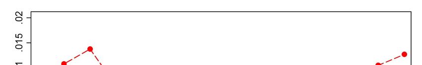
1 Introduction
Understanding the links between the weather, economic production and mortality has been
the focus of academic enquiry and policy debate for centuries. A large and distinguished
literature has focused on the role of adverse weather and production shortfalls in triggering
famines (Sen 1981). In developed countries and the majority of developing countries these
mass starvation events have been consigned to history. Structural change and industrializa-
tion in the developed nations means that citizens depend very little on weather contingent
production activities and can also marshall considerable resources to protect themselves
against the direct effects of adverse weather conditions. In these countries the power of
weather to result in excess mortality is extremely limited as has been confirmed by recent
analysis in countries like the US (Deschenes and Greenstone 2008).
The situation in developing and, in particular, poor developing countries is very differ-
ent. Here large swathes of the population continue to depend on weather-contingent agri-
cultural incomes. Households and communities in these settings have developed a range of
mechanisms to smooth consumption across income downturns (Townsend 1994). But these
localized forms of informal insurance may not offer much protection in the case of weather
shocks which affect the majority of citizens across a range of rural communities. Protection
afforded by the state is also often limited. In these settings weather shocks which interrupt
production and dent incomes may still have the power to increase mortality.1
The purpose of this paper is to find out whether this is the case or not by conducting the
first large-scale investigation into this phenomenon. To do this we take a large, developing
country – India. We assemble over forty years of daily temperature and rainfall records at
the district level and relate these to annual observations of mortality. Our main finding is
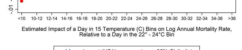
illustrated in Figure 1. The two lines show, for the USA and India respectively, the impact
of having an extra day whose daily mean temperature lies in each of fifteen temperature
bins relative to a day in the ‘reference’ bin of 22◦ -24◦ C (∼ 72◦ -75◦ F).2 As can be seen
in the figure, interannual variation in temperature in the US shows only a very weak co-
movement with the mortality rate. By strict contrast, hot days in India appear to lead to
significantly more death. Mortality increases steeply when there are more days at or above
the 30◦ -32◦ C (∼ 86◦ -90◦ F) range, relative to the 22◦ -24◦ C range. And these effects are
large—for example, one single additional day with a mean temperature above 36◦ C, relative
to a day with a mean temperature in the 22◦ -24◦ C range, increases the annual mortality rate
by roughly 0.75 %. Accross the subcontinent, relatively hot years have many more of these
1
The extensive literature which finds that levels of undernutrition and ill-health are extremely high in
rural populations that depend on agriculture also points in this direction.
2
The blue line comes from analysis using US counties (Deschenes and Greenstone 2008).
1lethal days, as we detail below.
Put simply, hot weather is a major source of excess mortality in India but not in the US.
To better understand why this is the case we first split out mortality observations into those
observed for rural and urban populations of Indian districts. This allows us to understand
whether or not the weather-death relationship is different for populations that are more or
less dependent on weather contingent forms of economic production. The high frequency
of our weather data also allows us to examine if weather during the growing season affects
mortality differently from weather in the non-growing season. We also gather data on output,
wages and prices for both urban and rural parts of districts in order to dig into the channels
via which weather might affect death.
The results we uncover suggest weather in India kills by denting agricultural incomes
via the interruptions it imposes on agricultural production and employment. We observe no
effect of weather on death in urban areas of India. This is true even for infants. All the effects
we observe in Figure 1 are coming through effects in rural areas. And it is only the weather
in the growing season that leads to higher death rates despite the fact that the non-growing
season in India is the hottest period of the year. Finally hot weather is associated with low
agricultural yields, lower agricultural wages and higher agricultural prices. Yields and wages
exhibit a pattern which is the inverse of that shown in Figure 1 where having more days
at or above the 30◦ -32◦ C range (relative to 22◦ -24◦ C) is associated with significantly lower
wages and yields. These results suggest that weather variation plays an important role in
the economic lives and health status of India’s rural citizens.
An important finding from the paper is that the structure of production and employment
mediates the impact of weather on death. This is the motivation for looking seperately at
effects on rural and urban populations in the same Indian district and at the effects of
weather during the growing and non-growing seasons in rural areas. In our analysis rural
and urban populations experience the same weather. However, it is only in the former that
we see downturns in output, incomes, wages and increases in prices. And moreover, these
effects are only the result of weather during the growing season. And it is inclement weather
precisely during this period that is driving up mortality in rural but not urban populations
within districts. Weather during the non-growing season which is the hottest, driest part of
the year does not affect mortality in either rural or urban areas. Thus though much of the
literature in developed countries has focussed on heat stress leading to excess mortality our
results suggest that agricultural incomes represent a key channel via which hot weather (and
deficient rainfall) affects death in poor, developing countries like India.
Our results match well with an extensive development literature on lean or hungry seasons
(Khandker 2009). This literature documents that malnutrition and morbidity are highest
2in the run-up to the post-monsoon harvest when food stocks are depleted, demand for
labor and agricultural wages are low, and food prices are high. Abnormally hot weather
during this period (particularly days above the 32◦ -34◦ C) limit the formation of grains in
key crops such as rice and therefore negatively affects the sizes of harvest and accentuate
income downturns for those dependent on agriculture. These effects are magnfied if rainfall
is also scant. Therefore hot weather (and deficient rainfall) can be particularly damaging
for agricultural incomes, wages and prices during the post-monsoon growing season which is
precisely what we find in our data. A variety of behaviours have evolved to deal with weather
shocks during the lean season – running down food stocks and other assets (e.g. savings,
livestock), borrowing money, forward selling labor and migrating have all been documented
in the literature. But our results suggest that the poorest, rural residents (e.g. landless
laborers) may be unable to fully withstand these income shocks and and as a result excess
mortalty results. And morevoer the mortality effects of growing season weather shocks
appear to persistent in the sense that abnormally hot weather in previous years’ growing
seasons adversely affects mortality in the current year though this effect dies out over time.
Famines may have indeed come to an end in India. However, our results suggest that
citizens or rural India still live in a world where inclement weather can significantly elevate
mortality. The fact that the weather may become more inclement via global warming is
then likely to pose particular challenges in these poor, rural settings. In a final section of
this paper we use our estimated coefficients of the within-sample (1957-2000) temperature-
death relationship in India to investigate the mortality predictions implied by two leading
climatological models of climate change. Our within-sample mortality estimates suggest
an increase in the overall Indian annual mortality rate of approximately 12% to 46% by
the end of the century. The estimated increase in rural areas ranges between 21% and
62%. As a reference point, a similar exercise performed on the United States suggests that
climate change will lead to a roughly 2% increase in the mortality rate there by the end of
the century. We fully expect rural Indians to adapt to an anticipated and slowly warming
climate in various ways and so these should be viewed as upper bound estimates. But the
direction of travel is nonetheless worrying and the fact that rural Indian citizens are already
not fully protected from the effects of weather implies that much more careful thinking has to
be applied to understanding how such protection might be afforded. And our results suggest
that calls for workable solutions are likely to need to become more urgent and strident as
global warming proceeds.
The remainder of this paper proceeds as follows. The next section outlines a theoretical
framework that describes the mechanisms through which weather might be expected to
lead to death. Section 3 describes the background features of India in our sample period
3from 1957-2000, as well as the data on weather, death and economic variables that we
have collected in order to conduct our analysis. Section 4 outlines our empirical method.
Section 5 presents results of the weather-death and weather-income relationships. Section
6 discusses what these estimates imply for predicted climate change scenarios in India, and
finally Section 7 concludes.
2 Conceptual Framework
In this section we discuss the potential mechanisms through which weather extremes could
lead to excess mortality in developing countries. The goal is to elucidate two potential
mechanisms: a ‘direct’ channel, in which human health suffers because of extreme weather
conditions that put human physiology under stress or exacerbate the disease environment,
and an ‘income-based’ channel, in which human health suffers because of the stress placed on
physiology, on which agents’ real incomes may depend. To capture both of these potential
channels relating weather to death, we develop a theoretical framework in which households
face both ‘direct’ health shocks due to temperature extremes as well as lower income due
to temperature extremes. In this model, an extension of Becker (2007), households can
choose to spend a share of their scarce income on health-improving goods that enhance the
probability of survival in the face of extreme temperatures.
Consider a representative agent who is potentially infinitely-lived. However, the agent
faces some probability of death in any period—the probability of the agent being alive in
period t having survived up to period t − 1 is given by the conditional probability of survival,
st ≤ 1. The agent derives utility in period t from consumption ct according to the intra-
temporal utility (or felicity) function, u(ct ). Finally, we asume that the agent discounts each
future period with a constant discount factor β < 1. Given all of this, the agent obtains an
expected value of lifetime utility given by
" ∞ t
! #
X Y
V =E βt st0 u(ct ) . (1)
t=0 t0 =0
Qt
Note that here, the term t0 =0 st0 is equal to the probability of the agent being alive in
period t.
We now endogenize the conditional probability of survival, st . Let st = s(ht , Tt ), where
ht is the amount of health-improving inputs that are consumed by the agent and Tt is a
variable (possibly multivariate) that captures the weather in period t. We assume that the
function s(ht , Tt ) is increasing and concave in ht , and we define Tt such that st is decreasing
in Tt .
4Crucial to this framework is the assumption that ht is a choice variable that is under the
agent’s control (subject to a budget constraint). Note that, in this formulation, there are
two types of goods. Consumption goods (denoted by ct ) are goods that the agent values
directly—they enhance the agent’s quality of life and are the sole argument in the utility
function, u(ct ). Health input goods (denoted by ht ) are valued only because they improve
the likelihood of survival in the current period and in future periods. We provide some
examples of health input goods, especially those that are important in our context, below.
The fact that the weather Tt affects that conditional probability of survival directly
(ie st = s(ht , Tt )) allows for the direct effect relating weather to mortality. The weather
Tt is assumed to be out of the agent’s control. Holding health inputs ht constant, high
temperatures can cause death (decrease survival chances st ) directly. An extensive public
health literature discusses the potential direct effects of high temperatures on human health
(see, for example, Basu and Samet (2002) for a comprehensive review).3 Periods of excess
temperature place additional stress on cardiovascular and respiratory systems due to the
demands of body temperature regulation. This stress is known to impact on the elderly and
the very young with particular severity, and can, in extreme cases, lead to death (Klineberg
2002, Huynen, Martents, Schram, Weijenberg, and Kunst 2001). An alternative ‘direct’ effect
of extreme weathers on death in India could include the possibility that disease pathogens
(for example, diarrhoeal diseases) thrive in hot and wet conditions, or that some vectors
of disease transmission (such as mosquitoes in the case of malaria) thrive in hot and wet
environments. We collapse all of these potential ‘direct’ channels into the possibility that
some index of temperature Tt enters the function s(ht , Tt ) directly (and negatively).
To allow for an ‘income-based channel’ through which weather extremes can cause death,
we include the possibility that the agent’s income is a function of the weather: yt = y(Tt ).
This is extremely likely in rural areas where incomes depend on agriculture directly or
indirectly. For simplicity, we assume that the weather variable Tt potentially affects both
income and survival in the same direction, such that y is decreasing in T . Because incomes are
observable the weather-to-income relationship is one that we are able to estimate. Naturally,
we expect this relationship to be minimal or even absent in urban areas. In contrast,
following well-known effects in the agronomic literature, as well as the literature on expected
effects of hotter climates on Indian agriculture (eg Kumar, Kumar, Ashrit, Deshpande,
and Hansen (2004) and Guiteras (2008)), we expect a strong negative relationship between
3
Extremely cold temperatures can also affect human health adversely through cardiovascular stress due
to vasoconstriction and increased blood viscosity. Deschnes and Moretti (2009) find evidence for a moderate
effect of extreme cold days on mortality (especially among the elderly) in the United States, though this
effect is concentrated among days below 10◦ F (ie −12◦ C). Days in this temperature range are extremely
rare in India.
5incomes in rural areas (ie agricultural incomes) and temperatures.
An income shortage caused by weather extremes could lead to death if this shortage
forces the agent to cut back on health input goods, ht . We take a broad view of these health
input goods, which the poor may struggle to afford even at the best of times, nevermind
those periods when weather extremes have caused income shortages. These could include
traditional health goods such as medicine or visits to a health center. Equally, they could
include the subsistence component of food consumption (that which increases the likelihood
of survival but is not valued in u(c) directly). Or given our focus on temperature an important
‘health good’ might be the use of air conditioning. More broadly, this ‘health good’ could
also encompass any leisure or rest (ie foregone labor, or income-earning opportunities) that
the agent might decide to ‘purchase’ so as to improve his health. This could include the
decision to work indoors rather than outdoors when it is hot, or to accept an inferior paying
job so as to avoid working outside on a hot day.
Finally, we specify the timing through which the uncertainty is resolved through time.
At the beginning of a period (for example, period t = 0), the temperature in the current
period (eg T0 ) is drawn. The agent then makes his choices in the current period (ie c0 and
h0 ) as a function of the current temperature (ie c0 = c0 (T0 ) and h0 = h0 (T0 )). After the
agent’s decision has been made, the agent’s death shock arrives (ie, having survived up to
date 0, the agent survives with probability s0 = s(h0 , T0 ).) Finally, if the agent survives this
death shock he enjoys intra-period utility u(c0 ) and the next period begins. If the agent
dies in period 0 then he enjoys no utility from this period (though the assumption of zero
utility in death is merely a normalization).
We specify the agent’s budget constraint as follows. We assume that the price of the
consumption good ct is pc and that of the health input good ht is ph ; this relative price
governs intra-temporal decisions. For simplicity we assume these prices are constant over
time. We also assume, for simplicity, that agents are able to borrow or save across periods
at the interest rate r (which is assumed to be constant, for simplicity) and that the agent
has access to a complete and fair annuity market (the only role of which is to simplify the
presentation of the lifetime budget constraint by ruling out the possibility that the agent
lives longer than expected and runs out of resources, or that the agent dies early when in
debt).
Under the above assumptions the agent’s inter-temporal budget constraint, starting from
period 0, can be written as:
" ∞ t
! #
X Y
s0 [y(T0 ) − pc c0 − ph h0 ] = E R−t st0 (pc ct + ph ht − y(Tt )) , (2)
t=1 t0 =0
6where R = (1 + r). That is, if total expenditure in period 0 (ie pc c0 + ph h0 ) exceeds income
in period 0, y(T0 ), then this must be funded by future surpluses.
An agent who maximizes lifetime utility, equation (1), subject to his lifetime budget con-
straint, equation (2), from the perspective of period 0 after T0 is known will make choices that
satisfy the following necessary first-order conditions for optimization. First, his allocation
of consumption across time will satisfy a standard Euler equation:
βRE [s1 u0 (c1 )]
u0 (c0 ) = .
E[s1 ]
This result states that the marginal utility of consumption in period 0 will be equal to the
expected marginal utility of consumption in the next period, times the opportunity cost
of consumption in the next period. This is the standard Euler equation adjusted for the
fact that the marginal utility of consumption in period 1 (ie u0 (c1 )) will only bring utility
if the agent survives (ie s1 = 1), and adjusted also for the fact that opportunity cost of
consumption in period 0 is also reduced by the possibility of non-survial (ie s1can derive an equation for the change in health spending across periods 0 and 1 which is
analogous to the consumption Euler equation presented above. This health input Euler
equation is: " ∂s V #
1 1
∂s0 V0 ∂h s1 λ
E = βRE . (3)
∂h λs0 1 + ∂s 1 W1
∂h s1
Here, V1 is the value of being alive at the start of period 1, and W1 is the agent’s net
asset position at the start of period 1. To gain intuition for this equation, imagine that the
agent’s net asset position at the start of period 1 is zero (ie W1 = 0), just as it was (by
normalization) at the start of period 0. In such a setting, this health input Euler equation is
entirely analogous to the consumption Euler equation introduced earlier: up to the dynamic
adjustment factor βR (which trades off the agent’s taste for impatience β with the returns to
saving R), the agent tries to equalize the expected marginal value of health spending across
periods. Since the maginal value of health spending is given by the product of the marginal
∂s V
effect of health saving on survival ( ∂h ) and the value of survival (the VSL, sλ ), the result in
equation (3) follows. More generally, W1 may not equal zero. But this simply adjusts the
above intuition for the fact that the agent does not want to risk dying with assets unspent.
This last result, the health spending Euler equation in equation (3), suggests that we
should expect a great deal of smoothing, not only in health expenditure but also in the
probability of survival itself. For a potentially long lived agent, the value of life at date 0
should be close to that at date 1, as long as the probability of death is being smoothed over
∂s
time. And since (by assumption) the marginal effect of health expenditure on survival ( ∂h )
is strictly decreasing in h, equation (3) suggests that we should expect the agent to be trying
to smooth (again, up to the adjustment factor βR) expected health expenditures h as well
as the expected value of life.
A final implication of the above first-order conditions is that they can be used to charac-
terize the agent’s willingness to pay (WTP) to avoid a worsening in the weather (∆T0 > 0)
in period 0. One way to derive the WTP is to imagine a transfer that varies as a function
of the observed weather T0 in period 0 and is designed to hold expected lifetime income V
constant for any value of T0 . Denote this transfer y ∗ (T0 ). It is then straightforward to show
that this transfer scheme will vary with T0 in the following manner:
dy ∗ (T0 )
dy(T0 ) ∂h0 ds(h0 , T0 ) V0
=− + − E . (4)
dT0 dT0 ∂T0 dT0 s0 λ
This expression, which characterizes the agent’s willingness to pay to avoid a small wors-
ening in the weather dT0 , is intuitive. WTP is the sum of three terms in this model. First,
since weather increases may adversely affect incomes directly (the ‘income-based channel’)
8the WTP first requires compensation for any loss of income caused by worse weather (ie a
payment of − dy(T
dT0
0)
, which we expect to be positive if bad weather leads to lower incomes).
Second, since inclement weather causes the agent to spend resources on health inputs that
have no direct utility benefits, the WTP requires the agent to be compensated for any change
in expenditures on health inputs caused by the worsening in the weather (ie a payment of
∂h0
∂T0
, which we expect to be positive if there is a direct effect of weather extremes on survival
chances that the agent is attempting to offset through the purchase of the heath good). The
final term in this WTP expression compensates the agent for the heightened risk of hdeath i
caused by inclement weather. Such a compensation requires a payment of − ds(hdT00,T0 ) E sV00λ ,
which is the product of the total effect of weather extremes on survival chances (ie ds(hdT00,T0 ) )
h i
and the dollar value of survival in period 0, E sV00λ , often referred to as the ‘value of a
statistical life’. The fact that this expression depends on the total deriviative of survival
with respect to weather, ds(hdT00,T0 ) , rather than the partial deriviative holding the health input
constant, is attractive from an empirical perspective.
It is important to note that all of the terms in the WTP expression in equation (4) are
potentially observable. Our empirical analysis below will aim to estimate both the the
reduced-form (or ‘total’) effect of weather extremes on death, ie ds(hdT00,T0 ) , and the effect of
weather extremes on income, ie dy(T dT0
0)
. Armed with these two essential ingredients and an
h i
estimate of the value of a statistical life in our setting (ie E sV00λ ) we will therefore be able
to estimate a lower bound on the agent’s willingness to pay to avoid a small worsening of
the weather, dT0 . This estimate will be a lower bound on the WTP because of our inability
to observe the full vector of health inputs that households are purchasing, and hence our
∂h0
inability to estimate ∂T 0
.
An important lesson from the WTP expression in equation (4) is that, in this model,
because money is fungible, it is irrelevant whether the agent suffers a heightened risk of
death due to weather extremes because of a ‘direct’ effect of bad weather on death or an
‘income-based’ effect. In either case, the agent has a well-defined willingness to pay to avoid
a inclement weather that is given by our WTP expression. This fact informs our empirical
approach which is centered on estimating two important ingredients that are required to
obtain bounds on the agent’s WTP, the reduced-form effect of weather on death (ie ds(hdT00,T0 ) )
and the effect of weather on incomes (ie dy(T dT0
0)
).
We conclude with a final word about policy in this environment. There are no market
failures in the above model—though it is clearly easy to imagine extensions to the model that
would involve plausible market failures, most notably constraints on the ability of agents to
borrow across periods without any restraint other than the inter-temporal budget constraint.
The absence of market failures implies no role for a self-funded policy here—a policy-maker
9facing the same constraints as the agent could do no better than the agent is doing himself.
But the WTP expression above does characterize the value that households place on avoiding
temperature extremes, which an external funder, such as a foreign donor, might wish to use
to compare the merits of competing policy proposals.
3 Background and Data
To implement the analysis in this paper, we have collected the most detailed and compre-
hensive district-level data available from India on the variables that the above conceptual
framework in Section 2 suggests are important. These variables include demographic vari-
ables (population, mortality and births), and variables that capture key features of India’s
urban and rural economies (output, prices and wages). We then study the relationship be-
tween these data and high-frequency daily data on historical weather that we have assembled.
In this section we describe these data, their summary statistics, and the essential features of
the background economy they describe.
Throughout this paper we draw heavily on the implications of the differential weather-
death relationship in urban and rural areas. We therefore begin with a short discussion of the
essential differences between these regions. Despite the dramatic extent to which the world
has urbanized in the last sixty years, the extent of urbanization in India has been relatively
slow: even in 2001, 72.2 percent of Indians lived in rural areas. The overriding distinction
between economic life in rural and urban India is the source of residents’ incomes. 76 % of
rural citizens belong to households that draw their primary incomes from employment in the
agricultural sector, while only 7 % of those in urban areas do so. Another distinction between
rural and urban areas lies in their consumption of food—that is, in their exposure to fluc-
tuations in the prices of foodstuffs. Deaton and Dreze (2009) draw on consumption surveys
to report that in 2001, 58 % of the average rural residents’ budget was spent on food, while
only 45 % of the average urban budget was devoted to food. Naturally, these consumption
differences may represent differences in the level of household per capita incomes between
rural and urban areas. Urban households are, on average, richer than rural households: in
2001 urban residents were 69 % richer on average than rural residents, according to Deaton
and Dreze (2009).
3.1 Data on Mortality and Population
The cornerstone of the analysis in this paper is district mortality data taken from the Vital
Statistics of India (VSI) publications for 1957-2000, which were digitized for this project.
10The VSI data represent the universe of registered deaths in each year and registration was
compulsory in India throughout our sample period. This source contains the most detailed
possible panel of district-level mortality for all Indian citizens.
Death tallies in the VSI are presented for infants (deaths under the age of one) and for
all others (deaths over the age of one), by rural and urban areas separately.4 From this
information we construct two measures of mortality: an infant mortality rate, defined as the
number of deaths under the age of one per 1000 live births; and an ‘all ages’ mortality rate,
defined as the total number of deaths over the age of one normalized by the population in
1000s.
Table 1 (which contains all of the summary statistics for data used in this paper) sum-
marizes the VSI data from the 1957-2000 period that we use in this paper, which comprise
315 districts spanning 15 of India’s largest states (and account for over 85 % of India’s pop-
ulation).5 The table reveals that measured mortality rates are high throughout this period.
For example, the average infant mortality rate is 40.5 per 1,000 live births. Geographi-
cally, average infant mortality rates range from 17.7 per 1,000 in Kerala to 71.3 per 1,000
in Orissa, revealing the substantial heterogeneity. As a basis of comparison, the mean US
infant mortality rate over these years was roughly 12 per 1,000. The Indian overall mortality
rate was 6.6 per 1,000. It is important to stress that these mortality rates are almost surely
underestimates of the extent of mortality in India. Despite compulsory registration of births
and deaths, many areas of the country suffer from significant under-reporting.6
Table 1 also documents the time variation in the two mortality rates. There is a remark-
able decline in both mortality rates in both rural and urban regions. For example, the overall
mortality rate declines from roughly 12 in 1957 to about 4 in rural areas and 6 in urban
areas by 2000. The decline in the infant mortality rate is also impressive, going from about
100 per 1,000 in 1957 to roughly 13.5 per 1,000 in 2000. In Section 4 below, we describe
our strategy to avoid confounding these trends in mortality rates with any time trends in
4
The rural/urban assignment is based on the following criteria, used throughout official Indian statistics:
urban areas comprise “(a) all places with a Municipality, Corporation or Cantonment or Notified Town Area;
and (b) all other places which satisfied the following criteria: (i) a minimum population of 5,000, (ii) at least
75% of the male working population was non-agricultural, and (iii) a density of population of at least 400
per sq. Km. (i.e. 1000 per sq. Mile).”
5
These states are (in 1961 borders and names): Andhra Pradesh, Bihar, Gujarat, Himachal Pradesh,
Jammu and Kashmir, Kerala, Madhya Pradesh, Madras, Maharashtra, Mysore, Orissa, Punjab, Rajasthan,
Uttar Pradesh, and West Bengal. These are the states with a consistent time series of observations in the
VSI data. The results in this paper are largely insensitive to the inclusion of all observations in the VSI
data.
6
According to the National Commission on Population of India, only 55 % of the births and 46 % of the
deaths were being registered in 2000. These estimates were obtained from India’s Sample Registration Sys-
tem, which administers an annual survey of vital events to a nationally representative sample of households.
The data published by the SRS, however, are only available at the state level.
11temperatures.
3.2 Data on Weather
A key finding from Deschenes and Greenstone (2008) is that a careful analysis of the relation-
ship between mortality and temperature requires daily temperature data. This is because
the relationship between mortality and temperature is highly nonlinear and the nonlinear-
ities would be missed with annual or even monthly temperature averages. This message is
echoed in the agronomic and agricultural economics literatures (as emphasized, for example,
by Deschenes and Greenstone (2007) and Schlenker and Roberts (2008)).
Although India has a system of thousands of weather stations with daily readings dating
back to the 19th century, the geographic coverage of stations that report publicly available
temperature readings is poor (and surprisingly the public availability of data from these
stations drops precipitously after 1970). Further, there are many missing values in the
publicly available series so the application of a selection rule that requires observations from
365 days out of the year would yield a database with very few observations.
As a solution, we follow Guiteras (2008) and use data from a gridded daily dataset that
uses non-public data and sophisticated climate models to construct daily temperature and
precipitation records for 1◦ (latitude) × 1◦ (longitude) grid points (excluding ocean sites).
This data set, called NCC (NCEP/NCAR Corrected by CRU), is produced by the Climactic
Research Unit, the National Center for Environmental Prediction / National Center for
Atmospheric Research and the Laboratoire de Météorologie Dynamique, CNRS. These data
provide a complete record for daily average temperatures and total precipitation for the
period 1950-2000. We match these gridpoints to each of the districts in our sample by
taking weighted averages of the daily mean temperature and total precipitation variables
for all grid points within 100 KM of each district’s geographic center. The weights are the
inverse of the squared distance from the district center.7
To capture the distribution of daily temperature variation within a year, we use two
different variables. The first of these temperature variables assigns each district’s daily
mean temperature realization to one of fifteen temperature categories—as already seen in
Figure 1. These categories are defined to include daily mean temperature less than 10◦ C
(50◦ F), greater than 36◦ C (96.8◦ F), and the thirteen 2◦ C-wide bins in between. The 365
7
On average, there are 1.9 grid points within a 100 km radius circles. The subsequent results are insensitive
to taking weighted averages across grid points across distances longer than 100 km and using alternative
weights (e.g., the distance, rather than the squared distance). After the inverse distance weighting procedure,
339 out of a possible 342 districts have a complete weather data record. The three districts that are dropped
in this procedure are Alleppey (Kerala), Laccadive, Minicoy, and Amindivi Islands, and the Nicobar and
Andaman Islands.
12daily weather realizations within a year are then distributed over these fifteen bins. This
binning of the data preserves the daily variation in temperatures, which is an improvement
over previous research on the relationship between weather and death that obscures much
of the variation in temperature.
Figure 2 illustrates the average variation in daily temperature readings across the fifteen
temperature categories or bins over the 1957-2000 period. The height of each bar corresponds
to the mean number of days that the average person in the vital statistics data (described
below) experiences in each bin; this is calculated as the weighted average across district-by-
year realizations, where the district-by-year’s total population is the weight. The average
number of days in the modal bin of 26◦ -28◦ C is 72.9. The mean number of days at the
endpoints is 3.7 for the less than 10◦ C bin and 3.4 for the greater than 36◦ C bin.
As a second approach to capturing the influence of temperature, we draw on a stark
non-linearity in the relationship between daily temperatures and both human and plant
physiology that is well known in the public health and agronomy literatures: temperatures
above (approximately) 32◦ C are particularly severe. We therefore construct a measure
of the cumulative number of degrees-times-days that exceed 32◦ C in a district and year.
This ‘degree-days’ measure has the advantage of collapsing a year’s 365 daily temperature
readings down to one single index, while still doing some justice to what is known about the
non-linear effects of temperature. Table 1 reports on summary statistics of this measure.
The national average is approximately 65 degree-days per year over 32◦ C, which implies an
average of just over two months during the year in which the daily mean temperature is at
34◦ C.
While the primary focus of our study is the effect of high temperatures on mortality,
we use data on rainfall to control for this potential confounding variable (to the extent
that temperature and rainfall are correlated). Table 1 reports annual precipitation totals.
However, the striking feature of rainfall in India is its intra-annual distribution: in an average
location, over 95 percent of annual rainfall arrives after the arrival of the southwest (summer)
monsoon, a stark arrival of rain on the southern tip of the subcontinent around June 1st which
then moves slowly northwards such that the northern-most region of India experiences the
arrival of the monsoon by the start of July—see, for example, Wang (2006). Naturally this
stark arrival of rainfall after a period of dryness triggers the start of the agricultural season
in India. We exploit this feature of the timing in our analysis below.
133.3 Data on Economic Outcomes in Rural India
3.3.1 Agricultural Yields
It is natural to expect that the weather plays an important role in the agricultural economy
in India. In turn, the agricultural economy may play an important role in the health of rural
citizens who draw their incomes from agriculture. To shed light on these relationships we
draw on the best available district-level agricultural data in India. The data on agricultural
outputs, prices, wages, and employment come from the ‘India Agriculture and Climate Data
Set’, which was prepared by the World Bank.8 This file contains detailed district-level data
from the Indian Ministry of Agriculture and other official sources from 1956 to 1986. From
this source we utilize three distinct variables on the agricultural economy: yields, prices, and
wages.
We construct a measure of annual, district-level yields by aggregating over the output
of each of the 27 crops covered in the World Bank dataset (these crops accounted for over
95 percent of agricultural output in 1986). To do this we first create a measure of real
agricultural output for each year (using the price index discussed below) and then divide
this by the total amount of cultivated area in the district-year. Table 1 reports on the
resulting yield measure for the 271 districts contained in the World Bank dataset, over the
period from 1956 to 1987. All of the major agricultural states are included in the database,
with the exceptions of Kerala and Assam.
3.3.2 Agricultural Prices
Because rural households spend so much of their budgets on food, food prices are an im-
portant determinant of rural welfare in India. We construct an agricultural price index for
each district and year which attempts to provide a simple proxy for the real cost of pur-
chasing food in each district-year relative to a base year. Our simple price index weights
each crop’s price (across the 27 crops in the World Bank sample) by the average value of
district output of that crop over the period.9 Table 1 reports on the level of this price index
in rural India. (The price data used in the World Bank source are ‘farm harvest prices’, so
we prefer to interpret these as rural prices rather than urban prices.) These figures and their
accompanying standard deviations show that prices are not as variable over space and time
as the yield figures in Table 1, potentially reflecting a degree of market integration across
India’s districts (so that a market’s price is determined by supply conditions both locally
8
The lead authors are Apurva Sanghi, K.S. Kavi Kumar, and James W. McKinsey, Jr.
9
Annual, district-level consumption data, which would be required to construct a more appropriate con-
sumption-based price index, are not available in India.
14and further afield).
3.3.3 Real Agricultural Wages
A second important metric of rural incomes (in addition to agricultural productivity, dis-
cussed above) is the daily wage rate earned by agricultural laborers. The World Bank dataset
contains information on daily wages, as collected by government surveys of randomly chosen
villages in each district and year. All figures are given in nominal wages per day, and are
then converted into equivalent daily rate to reflect the (low) degree of variation in the num-
ber of hours worked per day across the sample villages. We divide the reported, nominal
wage rate by the agricultural price index described above to construct an estimate of the
real rural agricultural wage in each district-year.10 As can be seen in Table 1, the level of
real wages is low throughout the period—never rising above 33.96 Rupees (base year 2000),
or approximately 2 US dollars (base year 2000) per day in PPP terms.
3.4 Data on Economic Outcomes in Urban India
As emphasized in Section 2, an important channel through which weather variation can
reduce welfare and lead to death is through household’s incomes. While it is natural to expect
strong effects of temperature extremes on rural, agricultural incomes, we also investigate the
extent to which economic conditions in urban areas react to temperature fluctuations. To
this end we have collected the best available data on urban economic conditions, and describe
the sources of that data here. It is important to stress at the outset that, perhaps because
of the over-riding current and historical importance of agriculture for economic welfare in
India, the statistics on India’s urban economy are not as detailed as those on India’s rural,
agricultural economy. All of the sources listed below report data on urban outcomes at the
state level, whereas all of the rural equivalents introduced above were available at the district
level.
3.4.1 Manufacturing Productivity
India’s manufacturing sector (especially its ‘registered’ or formal manufacturing sector) is
almost entirely located in urban areas. For this reason we use a measure of state-level
registered manufacturing productivity (real output per worker) as one measure of the pro-
ductivity of the urban area of each state in each year. We draw this data from Besley and
10
A better real wage measure would of course also incorporate price information on non-agricultural items
in the rural consumption basket. Unfortunately, the price and quantity information that would be required
to do this are unavailable annually at the district level in India.
15Burgess (2004), who collected the data from publications produced by India’s Annual Survey
of Industries.
3.4.2 Urban Consumer Price Index
Every year India’s statistical agencies produce two official consumer price indices, one in-
tended to be relevant for agricultural workers and one intended to be relevant for manufac-
turing workers. These are published by the Labour Bureau. The latter index is collected
(by the NSSO) from urban locations, and is based on weights drawn from NSS surveys of
manufacturing workers. We therefore follow standard practice and use on the manufacturing
workers’ CPI as a CPI that reflects urban prices. Data on this index is taken from Besley and
Burgess (2004), who collected the data from the annual Indian Labour Yearbook publication.
3.4.3 Real Manufacturing Wages
The final measure of incomes in urban areas that we exploit comes from manufacturing wage
data. To construct this variable we first use data on nominal (registered) manufacturing
wages, as surveyed by the Annual Survey of Industries and published in the annual Indian
Labour Yearbook, which was collected by Besley and Burgess (2004). We then divide nominal
manufacturing wages by the urban CPI variable introduced above to create a measure of
real manufacturing wages.
4 Methodology
In this section we describe the econometric method that we use to analyze the weather-death
relationship and accompanying relationships in this paper.
We pursue two different approaches to modeling the temperature-death relationship, but
our approach to the precipitation-death relationship is held constant throughout. Our first
approach to estimating the temperature-death relationship was introduced briefly in the
Introduction, and results based on it were presented in Figure 1, but we provide details here.
Our estimating equation uses a flexible specification to model the relationship between daily
temperature variation and annual mortality rates as follows:
X X
15
Ydt = θj=1 TMEANdtj + δk 1 {RAINdt in tercile k }
j k
+ αd + γt + λ1r t + λ2r t2 + εdt , (5)
where Ydt is the log mortality rate (or an alternative outcome variable such as an income
16measure) in district d in year t. We use the log of the death rate (or of alternative outcome
variables) in order to draw straightforward comparisons across different outcome variables,
but our results are largely unchanged if we instead use the level of the death rate (or alter-
native outcome) rather than its log as our dependent variable. The r subscript refers to a
‘climatic region’ (explained below). The last term in the equation is a stochastic error term,
εdt .
The key variables of interest here are those that capture the variation in daily temper-
atures in district d within year t. The variable T M EANdtj denotes the number of days in
district d and year t on which the daily mean temperature fell in the jth of the fifteen bins
used in Figure 2. We estimate separate coefficients θj for each of these temperature bins.
However, because the number of days in a standardized year always sums to 365 one of these
fifteen coefficients cannot be identified; we use the middle bin, that for temperatures between
22◦ C and 24◦ C, as a reference category whose coefficient is therefore normalized to zero.
This approach makes three assumptions about the effect of a day’s mortality impact
on the outcome variable. First, this approach assumes that the impact is governed by the
daily mean alone; since daily data on the intra-day (‘diurnal’) variation of temperatures in
India over this time period is unavailable to us, this assumption is unavoidable. Second,
our approach assumes that the impact of a day’s mean temperature on the annual mortality
rate is constant within 2◦ C degree intervals; our decision to estimate separate coefficients θj
on each of fifteen temperature bin coefficients represents an effort to allow the data, rather
than parametric assumptions, to determine the mortality-temperature relationship, while
also obtaining estimates that are precise enough that they have empirical content. This
degree of flexibility and freedom from parametric assumptions is only feasible because of the
use of district-level data from 44 years. Finally, by using as a regressor the number of days
in each bin we are assuming that the sequence of relatively hot and cold days is irrelevant for
how hot days affect the annual outcome variable. This is a testable assumption, for which
we find support. Specifically, including regressors that capture the presence of two or more
‘hot’ days (eg over 32◦ C) does not change our main results.
The second set of variables on the right-hand side of equation (5) aims to capture variation
in precipitation (essentially rainfall, given our sample restriction to non-Himalayan India).
Given that our primary focus is on the effects of temperature on death, the coefficients
on rainfall regressors are of secondary importance. However, because it is possible that
temperature variation is correlated with rainfall variation, the inclusion of these rainfall
variables is important. We model rainfall in a manner that is fundamentally different from
our approach to modeling temperature because of one key difference between temperature
and rainfall: rainfall is far more able to be stored (in the soil, in tanks and irrigation systems,
17and in stagnant water that might breed disease) than is temperature. Given this distinction,
while we have modeled the effect of temperature as the sum over daily impacts, we model
the effect of rainfall as the impact of sums over daily accumulations. The specific approach
pursued in equation (5) above uses regressors that aim to flexibly capture how a given
year’s total annual rainfall affects the outcome variable. To do this as simply as possible we
calculate whether the total amount of rainfall in year t in district d was in the upper, middle
or lower tercile of annual rainfall amounts in district d over all years in our sample; these
are the regressors 1 {RAINdt in tercile k }. We estimate a separate coefficient on each of the
three tercile regressors (though of course one of these regressors is omitted as a reference
category, which we take to be the middle tercile regressor).
The specification in equation (5) also includes a full set of district fixed effects, αd , which
absorb all unobserved district-specific time invariant determinants of the log mortality rate.
So, for example, permanent differences in the supply of medical facilities will not confound
the weather variables. The equation also includes unrestricted year effects, γt . These fixed
effects control for time-varying differences in the dependent variable that are common across
districts (for example, changes in health related to the 1991 economic reforms). The as-
sumption that shocks or time-varying factors that affect health are common across districts
is unlikely to be valid. Consequently, equation (5) includes separate quadratic time trends
for each of the five climatic regions r of India (groupings of states with similar climates
according to India’s Meteorological Department.)
Our second approach to modeling the temperature-death relationship estimates fewer
parameters while still doing some justice to the non-linear nature of this relationship. This
second approach, which we refer to as the ‘single-index’ approach, estimates the parameters
in:
3
X
Ydt = βCDD32dt + δk 1 {RAINdt in tercile k } + αd + γt + λ1r t + λ2r t2 + εdt , (6)
k=1
where the variable CDD32dt is the number of cumulative degree-days in district d and year
t that exceeded 32◦ C.11 This is a particular restriction on the flexible approach in equation
(5)—where the 13 temperature bin coefficients θj below 32◦ C are restricted to be zero and
the three coefficients above 32◦ C are restricted to be linearly increasing in their average
temperatures—for which we find some support below.
Our assumptions in pursuing this simplification are that: (i) on days during which the
mean temperature is below 32◦ C, temperature is irrelevant for determining the outcome
11
For example, if a given district-year had only two days over 32◦ C, one at 34◦ C and the other at 36◦ C,
its value of CDD32dt would be 6.
18variable (eg mortality) Ydt ; and (ii), the effect of days whose mean temperatures exceed 32◦
C is linearly increasing (at the rate β) in the mean daily temperature. This is broadly in
line with a large public health and agronomy literature that uses the cumulative degree-day
approach. The advantage of this single-index approach is that by estimating one coefficient
rather than 15 we have more statistical power for teasing out the heterogeneous effects of
temperature in order to learn more about the weather-death relationship.
The validity of this paper’s empirical exercise rests crucially on the assumption that
the estimation of equations (5) and (6) will produce unbiased estimates of the θj , β and
δk parameters. By conditioning on district fixed effects, year fixed effects, and quadratic
polynomial time trends specific to each climatic region, these parameters are identified from
district-specific deviations in weather about the district averages after controlling for the por-
tion of shocks that remains after adjustment for the year effects and cubic time polynomials.
Due to the randomness and unpredictability of weather fluctuations, it seems reasonable to
presume that this variation is orthogonal to unobserved determinants of mortality rates.
There are two further points about estimating equations (5) and (6) that bear noting.
First, it is likely that the error terms are correlated within districts over time. Consequently,
the paper reports standard errors that allow for heteroskedasticity of an unspecified form
and that are clustered at the district level. Second, we fit weighted versions of equations
(5) and (6), where the weight is the square root of the population in the district for two
complementary reasons.12 First, the estimates of mortality rates from large population
counties are more precise, so this weighting corrects for heteroskedasticity associated with
these differences in precision. Second, the results reveal the impact on the average person,
rather than on the average district, which we believe to be more meaningful.
5 Results
5.1 Weather and Death
Figure 1 in the Introduction of this paper displayed the result of running a regression of
weather on death for India and the US. The two lines in Figure 1 show the impact of
having an extra day in fifteen temperature bins relative to a day in the 22◦ -24◦ C bin
for the US and India respectively. That is, the fifteen coefficient estimates θbj for each of
fifteen temperature bins j from estimating equation (5) are presented graphically, under the
normalization that coefficient on the middle bin, the 22◦ -24◦ C bin, is zero. Further, as
12
When estimating relationships in which the outcome variable concerns agricultural income we weight by
the cultivated area of the district-year since the fundamental sampling unit in the data used to construct
these outcome variables is a parcel of land.
19discussed in Section 4, while only the coefficients on these fifteen temperature regressors are
plotted, these coefficients were estimated while controlling for rainfall variation, district and
year fixed effects, and quadratic polynomial trends for each climatological region. This is
also true for all further graphical presentations of estimates of equation (5) shown below, in
Figures 3 to 5.
As can be seen in Figure 1, interannual variation in temperature in the US shows no clear
relationship with mortality. In strict contrast having more hot days in India is associated
with significantly more death. Mortality increases steeply when there are more days at or
above the 30◦ -32◦ C range (relative to 22◦ -24◦ C). And the effects are large, for example,
one additional day with a mean temperature above 36◦ C, relative to a day with a mean
temperature in the 22◦ -24◦ C range, increases the annual mortality rate by roughly 0.75 %.
Put simply, hot weather kills in India but not—at least on nowhere near the same scale—in
the US.
To better understand why this is the case we first split out mortality observations into
those observed separately for the rural and urban populations of each Indian district. This
allows us to understand whether or not the weather-death relationship is different for popu-
lations that are more or less dependent on weather contigent forms of economic production.
The high frequency of our weather data also allows us to examine if weather during the
growing season affects mortality differently from weather in the non-growing season.
5.1.1 Urban versus Rural
In terms of economic structure, urban and rural India look very different. In employment
terms the rural areas of India are dominated by agriculture whilst urban areas are dominated
by services and manufacturing. As we have seperate observations of mortality for rural
and urban populations within the same district we can test whether the weather-death
relationship differs for these two populations.
The results from doing this are shown in Figures 3 and 4. These figures plot estimated
response functions between log annual mortality rate and temperature exposure, estimated
separately for urban and rural populations. These models pool across age groups and pertain
to the total population of a particular area within each district (i.e. the urban or rural
segment of a district).
Figure 3 shows the response function estimated from the urban population. For both the
urban Indian population and the US population there is, in effect, no significant relationship
between weather and death. The results are remarkably different from those in the rural
areas. The largest urban India coefficient is for the highest temperature bin (> 36◦ C), and
the magnitude is only 0.003—half the magnitude of the all-India coefficient (of 0.075) in
20You can also read