Anatomy-aided deep learning for medical image segmentation: a review - IOPscience
←
→
Page content transcription
If your browser does not render page correctly, please read the page content below

Physics in Medicine & Biology

TOPICAL REVIEW • OPEN ACCESS

Anatomy-aided deep learning for medical image segmentation: a review
To cite this article: Lu Liu et al 2021 Phys. Med. Biol. 66 11TR01

View the article online for updates and enhancements.

                                This content was downloaded from IP address 46.4.80.155 on 05/08/2021 at 11:58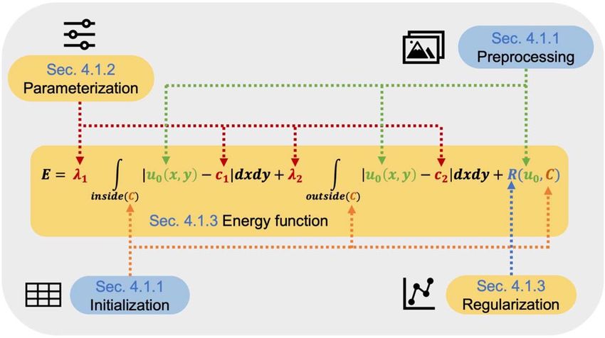
Phys. Med. Biol. 66 (2021) 11TR01                                                     https://doi.org/10.1088/1361-6560/abfbf4

                              TOPICAL REVIEW

                              Anatomy-aided deep learning for medical image segmentation: a
OPEN ACCESS
                              review
RECEIVED
19 January 2021
                              Lu Liu1,2 , Jelmer M Wolterink1 , Christoph Brune1                  and Raymond N J Veldhuis2
REVISED                       1
19 April 2021
                                  Applied Analysis, Department of Applied Mathematics, Faculty of Electrical Engineering, Mathematics and Computer Science,
                                  University of Twente, Drienerlolaan 5, 7522 NB, Enschede, The Netherlands
ACCEPTED FOR PUBLICATION      2
                                  Data Management and Biometrics, Department of Computer Science, Faculty of Electrical Engineering, Mathematics and Computer
27 April 2021
                                  Science, University of Twente, Drienerlolaan 5, 7522 NB, Enschede, The Netherlands
PUBLISHED
26 May 2021                   E-mail: l.liu-2@utwente.nl

                              Keywords: medical image segmentation, anatomical information, deep learning
Original content from this
work may be used under
the terms of the Creative
Commons Attribution 4.0
licence.
                              Abstract
Any further distribution of   Deep learning (DL) has become widely used for medical image segmentation in recent years. However,
this work must maintain
attribution to the
                              despite these advances, there are still problems for which DL-based segmentation fails. Recently, some
author(s) and the title of    DL approaches had a breakthrough by using anatomical information which is the crucial cue for
the work, journal citation
and DOI.                      manual segmentation. In this paper, we provide a review of anatomy-aided DL for medical image
                              segmentation which covers systematically summarized anatomical information categories and
                              corresponding representation methods. We address known and potentially solvable challenges in
                              anatomy-aided DL and present a categorized methodology overview on using anatomical information
                              with DL from over 70 papers. Finally, we discuss the strengths and limitations of the current anatomy-
                              aided DL approaches and suggest potential future work.

                              1. Introduction

                              Generally, segmentation is defined as an operation that separates images into several parts with different
                              meanings. In the medical field, segmentation as a method of medical imaging analysis is crucial for diagnosis and
                              treatment. As soon as computers could load medical images as digital files, multiple pieces of research have
                              explored systems for automated medical image segmentation. For medical images, segmentation is usually a
                              binary problem since only the parts of interest are important. It can also be multi-target segmentation if the
                              number of targets of interest is more than one.
                                   Initially, segmentation was done with mathematical models (e.g. Fuzzy C-mean clustering, K-means
                              clustering) and low-level pixel processing (e.g. region growing. edge detection methods, watershed) (Lee et al
                              2015). At the end of the 20th century, machine learning (ML) and pattern recognition techniques were applied to
                              segmentation using training data to develop a model. These supervised techniques are still very popular and
                              many commercial medical image analysis applications are based on them. The extracted features are designed or
                              selected by researchers in these approaches and referred to as handcrafted features. Although they are usually
                              human-understandable, they may not be ideal features for segmentation. Recently, with the development of
                              neural networks and deep learning (DL), computers can extract representative features from images. Many deep
                              neural networks for image processing are designed based on the concept that networks of many layers transform
                              input images to output labels by learning high-level features. The most representative type of model for image
                              analysis to date is the convolutional neural network (CNN). The CNN as an important model in has solved many
                              key commercial applications and showed its ability in many contests. In medical image analysis, the CNN and
                              other DL methods started to show their ability at many workshops, challenges, and conferences.
                                   As the number of papers increases rapidly, a few review papers are trying to summarize these applications.
                              There are general review papers on DL in medical image analysis published by Shen et al (2017) and Litjens et al
                              (2017). Review papers are focusing on medical image segmentation using DL published recently by Taghanaki
                              et al (2020), Haque and Neubert (2020), and Hesamian et al (2019). Some review papers have more specific

                              © 2021 Institute of Physics and Engineering in Medicine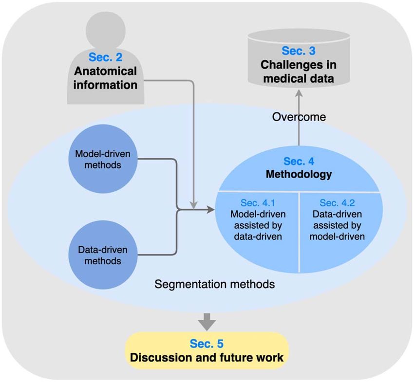
Phys. Med. Biol. 66 (2021) 11TR01                                                                            L Liu et al

focuses. For example, the work by Zhuang et al (2019) and Chen et al (2020a) summarized cardiac image
segmentation networks; Yi et al (2019) discussed the use of generative adversarial networks (GANs) in medical
imaging; Zhang et al (2019) focused on the small sample problem in biomedical image analysis; Karimi et al
(2020) explored the problem of noisy labels in medical image analysis; Tajbakhsh et al (2020) investigated DL
solutions for imperfect datasets in medical image segmentation; Cheplygina et al (2019) surveyed not-so-
supervised networks using semi-supervised, multi-instance and transfer learning in medical image analysis.
Jurdia et al (2020) categorized high-level prior-based loss functions for medical image segmentation according
to the nature of the prior: shape, size, topology, and the inter-region constraints. Bohlender et al (2021) reviewed
shape-constrained DL for medical image segmentation. Some review papers focus on specific segmentation
tasks in certain modalities. Yedavalli et al (2020) reviewed artificial intelligence in stroke imaging. Zhang et al
(2020a) surveyed DL methods for isointense infant brain segmentation in magnetic resonance imaging (MRI),
while Ma et al (2020) focused on liver tumor segmentation in computed tomography (CT) images. Vrtovec et al
(2020) explored the segmentation of organs at risk for head and neck radiotherapy planning. Ebrahimkhani et al
(2020) summarized segmentation methods of knee articular cartilage. As brain tumor segmentation is an active
topic, several review papers on this topic are published by Sun et al (2019), Hameurlaine and Moussaoui (2019),
Saman and Narayanan (2019), Jiang et al (2020), and Li et al (2020a). Feo and Giove (2019) reviewed
segmentation methods of small rodents brains, and Lin and Li (2019) reviewed brain segmentation methods
from multi-atlas to DL. Chen et al (2020b) summarized thyroid gland segmentation and thyroid nodule
segmentation methods for ultrasound images. Two recent reviews of retinal blood vessel segmentation are
published by Soomro et al (2019) and Samuel and Veeramalai (2020). From these review papers, we see that
there are many possibilities in this field and various review focuses indicates various research directions.
However, none of them focus on the use of anatomical information which is the main cue of segmentation for
experts. In some segmentation tasks, anatomical information is critical. For example, when experts segmenting
epicardial fat in CT images, as epicardial fat and paracardial fat have a very similar appearance, the pericardium is
the only thing separating the two fat tissues. But pericardium is rarely visible in CT images. Experts need
anatomy knowledge of the heart to estimate the pericardium and epicardial fat as well.
    In the very beginning, only experts who are experienced and have anatomical knowledge can do the
segmentation manually for medical images. Thus, ideally, the segmentation networks should mimic the experts
when predicting the labels for medical images. Considering that most of the segmentation networks are typically
trained with pixel-wise or voxel-wise loss functions (e.g. cross-entropy, dice losses), it may limit the ability to
learn features that is representative anatomically or structurally. Some of the above review papers mentioned the
use of anatomical information with examples and pointed out that applying anatomical constraints to networks
shows improved performance and robustness. However, they rarely analyze or summarize the use of anatomical
information in DL for medical image segmentation in depth. This review paper is made to fill this gap.
    Figure 1 illustrates the overview of this paper. In this paper, we provide an overview of state-of-the-art
anatomy-aided DL techniques for medical image segmentation by introducing various anatomical information
types (section 2), summarizing challenges in this field (section 3), summarizing and analyzing the methodology
of using anatomical information in DL (section 4) with its weaknesses, strengths, and uncertainty. At the end
(section 5), we discuss the strengths and weaknesses of anatomy-aided DL for medical image segmentation and
potential directions for future work.

2. Anatomical information

In this section, we introduce anatomical information of four categories: shape, appearance, motion, and context.
In general, human anatomy studies the morphology of the human body. Anatomy knowledge is concluded after
long-time observation of the human body or part of the human body. As the object of study and observation way
varies, the two main branches of human anatomy are gross anatomy and microscopic anatomy. Gross anatomy
studies anatomical structures that are obvious to the naked human eye such as body parts and organs. Nowadays,
many noninvasive techniques like MRI, CT, ultrasound (US), or x-ray are used to image inside the living body.
After the microscope was invented, people study minute anatomical structures such as tissues and cells with the
assistance of it. This is the so-called microscopic anatomy.
     For segmentation tasks in medical images, plenty of anatomical information is available. However, when
applying, we need to describe or model the information properly. For different objects, different information is
considered informative or useful to distinguish the target from other structures. Thus, not all anatomical
information can contribute. In the following subsections, we list the anatomical information that has been used
in medical image segmentation networks and introduce their ways of description.
     As shown in figure 2, anatomical information can be divided into four categories and the sub-categories are
listed as well.

                                               2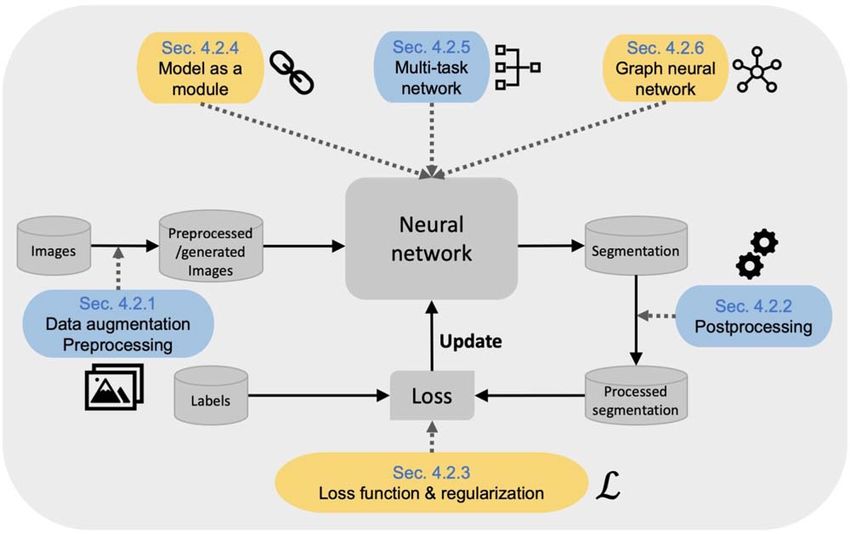
Phys. Med. Biol. 66 (2021) 11TR01                            L Liu et al

   Figure 1. Overview of the review paper.

   Figure 2. Overview of section 2 anatomical information.

                                                       3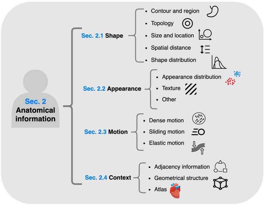
Phys. Med. Biol. 66 (2021) 11TR01                                                                             L Liu et al

2.1. Shape information
Shape information is a crucial descriptor for target objects in a medical image. For many segmentation targets,
the shape is a basic element for experts to distinguish the target from other structures. In this section, we discuss
shape information from five aspects: contour and region (section 2.1.1), topology (section 2.1.2), size and
location (section 2.1.3), spatial distance (section 2.1.4), and shape distribution (section 2.1.5).

2.1.1. Contour and region
There are mainly two ways to model the shape geometrically: parametric way and non-parametric way. Most
relatively regular shapes can be modeled parametrically. For example, 2D shapes like ellipse, circle, rectangular,
etc and 3D shapes like sphere, cylinder, cube, etc can be described with parameters like center coordinate, radius,
height, width, orientation, etc.
    For not-so-regular shapes, a non-parametric way like a level set (LS) representation may be a better
description. The idea of an LS representation is to represent contour C by a function j. The boundary C of an
object W̃ is defined as the zero set of j. i.e.
                                             C = {x Î W : j (x ) = 0},                                              (1)
where Ω denotes the entire image plane. The sign of f(x) determines whether x is in W̃ or outside W̃,

                                                   ⎧+ 1 if x is inW
                                                                  ˜
                                    sign (j (x )) = 0 if x is on the boundary .                                     (2)
                                                   ⎨
                                                                  ˜c
                                                   ⎩- 1 if x is inW
The LS representation is widely used in optimization-based segmentation methods, and it is particularly effective
for convex objects like optic cum and disc segmentation (Nosrati and Hamarneh 2016). With LS representation,
the active contour model (ACM) is widely used for image segmentation.
    ACM (or deformable model) is one of the conventional segmentation methods (McInerney and
Terzopoulos 1996, Jayadevappa et al 2011, Chen et al 2020a). Compared to basic models such as simple
thresholding, region-growing, or edge detection, ACMs have shown better performance and robustness.
Representative models are snakes (Kass et al 1988), the Mumford–Shah model (Mumford and Shah 1989), and
the active contour without edges (ACWE) (Chan and Vese 2001). Subsequently, many extensions and variations
of ACM tried to solve the problem efficiently. Examples of well-known solvers are dual projection and graph cut
(Morar et al 2012). These models formulate segmentation as an energy minimization problem. Variational
methods and partial differential equations (PDEs) are used to solve them.
    Most ACMs start with an initial guess boundary which is one or multiple closed contours. During the
process of energy minimization, the contour is modified to more accurate and closer to the desired boundary
under the constraints and a penalty given in the energy function. The common penalty terms control the
smoothness of the contour, and the curvature of the contour, etc. Based on the information used in the models,
there are two categories of ACMs-edge-based models and region-based models (Le et al 2020). Edge-based
models use image gradient as edge information to constrain the contour to the target boundary. A well-known
model in this category is the geodesic ACM (Caselles et al 1997). The ACWE model (Chan and Vese 2001) is an
example of region-based models. This model utilizes an LS representation for the contour of target objects.
Similar to most region-based models, its energy function consists of two parts: regularization and energy
minimization. It uses the statistical information inside and outside the boundary to guide the modification.
Since an image gradient is not involved, comparing to edge-based models, region-based models are more robust
against noise and better at detecting weak boundaries.
    Nowadays, the group of ACM methods is still growing. Many recent models have better performance than
years before and can handle many image segmentation problems. However, they have many limitations.
Generally, the segmentation results are obtained by minimizing a certain energy function using gradient descent
(Zhou et al 2013). Since most of the ACMs are not convex, the segmentation results may get stuck in local
minima. They are unstable when dealing with occluded images. There are many parameters chosen empirically.
The segmentation results rely on the parameters, number of iterations, and image quality. They may generate
unpredictable or wrong results when handling complex images. Especially, the accuracy decreases dramatically
with images in the wild.

2.1.2. Topology
Many anatomical objects in medical images have fixed topological characteristics that are supposed to be
maintained in the segmentation results. For example, when segmenting the airway wall in transverse CT slices,
the airway wall has a doughnut shape which needs to be preserved in the segmentation results. Topology studies
the properties of geometric objects that are invariant during continuous deformations in topological spaces. The
two main topological properties are connectivity and compactness. Connectivity describes whether an object is

                                                 4
Phys. Med. Biol. 66 (2021) 11TR01 L Liu et al
connected (e.g. one circle is connected, while two non-intersecting circles are not connected). Compactness
describes whether an object is closed and bounded (e.g. a circle is compact, while a line is not). There are many
tools from topological data analysis (TDA) to describe the topological characteristics. TDA relates topology and
geometry to extract information from datasets of high-dimension. The main tool of TDA is persistent homology
(PH). The review papers Wasserman (2018) and Chazal and Michel (2017) include fundamental and practical
aspects about TDA.
2.1.3. Size and location
Size and location are the most basic information of an object. In many cases, size and location can be used as a
constraint to filter or remove redundant and unrelated objects. Moreover, some segmentation methods using
shape priors may over-correct the segmentation results to make them fit the input shape prior. As an example,
when there are pathological cases in the input image, an abnormal part that deviates from the shape before, may
lead to healthy cases not being segmented correctly. Using size and location constraints may be an alternative to
reduce undesirable results (Nosrati and Hamarneh 2016).
The parameter for describing size varies as image modality or target changes. It could be the length, width,
height, area, and volume, etc. Similarly, there are many parameters for describing location such as coordinates,
and the centroid. In the case of having rough information about the size and location, soft constraints such as a
size range or a location range can be applied.
2.1.4. Spatial distance
There mainly two types of spatial distances that are relatively widely incorporated in segmentation methods:
minimum distance and maximum distance (Nosrati and Hamarneh 2016). The minimum distance between two
objects can be used as a constraint to enforce the separation of regions or objects. The maximum distance
between regions or boundaries is known in many cases. For example, in cardiac CT, the maximum distance
between the left ventricle and its myocardium can be estimated. Other types of spatial distance are derived from
minimum and maximum distance. In some cases, the distance between objects is supposed to be controlled in a
specific range. The idea of attractive force and repulsive force in physics could be used to model the spatial
relationships (Zeng et al 1998). More models can be used to control the distance between objects such as a
deformable model, etc. Since recently there is little work based on them for medical image segmentation, it is not
described in this article.
2.1.5. Shape distribution
In practice, target objects in medical image segmentation hardly have regular shapes. Most objects from different
sample images are not identical or rigid. Even relatively regular objects (in medical image segmentation) like
organs have various shapes from one to another. Thus, a fixed geometrical model may not be appropriate for
such objects. One way to handle such intra-class variation is to form a shape probability model by adding a
probability distribution to the model.
There are two parts in most of the shape probability models: shape representations and probability
distributions. For shape representations, there are many choices like the LS, point cloud, surface mesh, etc. For
probability distributions, common models are Gaussian distribution, Gaussian mixture model, etc.
2.2. Appearance information
Appearance is one of the most important and obvious visual information to distinguish various objects and
structures in medical images. Appearance is influenced by many factors such as intensity, color, brightness,
texture, and saturation. There are many ways to formulate appearance models for image segmentation. Here we
introduce appearance distributions, texture models, and other common ideas of extracting appearance
information.
2.2.1. Appearance distribution
The appearance distribution is usually learned or estimated by observing the distribution of appearance features
in small samples. Assuming that Fi(x) represents a set of appearance features of the object i and the probability
P(x|Fi(x)) of every pixel or voxel to each class is known, this is the appearance distribution. Examples of the most
direct appearance features are a gray-scale value, an RGB value, or other values of every pixel or voxel. To use the
distribution in segmentation networks, for example, we can force the segmentation distribution to fit the prior
distribution by minimizing the distance between them.
5Phys. Med. Biol. 66 (2021) 11TR01 L Liu et al
2.2.2. Texture
Texture in medical images is one of the direct visual cues to distinguish many objects such as tissues and lesions.
Many models are used to represent the texture of objects. Most of them are used in ML methods to represent
texture features, while some inspired research using DL for image segmentation.
The recent review on texture feature extraction methods (Humeau-Heurtier 2019) classified methods into
seven classes: statistical approaches, structure approaches, transform-based approaches, model-based
approaches, graph-based approaches, learning-based approaches, and entropy-based approaches. Many of the
texture features mentioned in the review have been used in medical image segmentation. Here we give several
examples. There are simple texture models. For example, the model proposed by Bigün et al (1991) utilizes the
Jacobian matrix and a Gaussian kernel to generate a three-channel texture feature. Some advanced texture
features are widely used in image segmentation before DL became the main trend. The group of texture features
based on Haar and Gabor filters has shown effectiveness in medical image segmentation (Santner et al 2009,
Yang et al 2014, Ibragimov et al 2017).
2.2.3. Other
Many other appearance features are extracted for image segmentation. For instance, the Fourier transformation,
a bag of visual words, the local binary pattern (LBP), the histogram of oriented gradient, the scale-invariant
feature transform, etc are used to extract appearance features (Nosrati and Hamarneh 2016). Appearance
features are mainly extracted from three domains: the spatial domain, the time domain, and the scale domain
(Nosrati and Hamarneh 2016). For different targets, different features can be selected or designed to reach better
segmentation performances. These appearance features that are designed manually are considered hand-crafted
features. Nowadays, with DL, segmentation networks can learn appearance features automatically.
2.3. Motion information
Life is in motion. There are three types of motion in our body for image analysis: the dense motion, the sliding
motion, and the elastic motion. A typical example of dense motion is the particle movement in the fluid. Applied
to medical images, it could be for example cells moving in blood or other fluid. The standard representation of
dense motion in computer vision is the optical flow (Szeliski 2010). Another basic motion type is the sliding
motion. Usually, physical models with velocity and locations are used to describe such motion. Elastic motion is
the deformation of objects caused by force. There are many physical models available for describing various
motion types. However, as the human body is complex, it is not easy to capture and utilize proper motion
information for assisting medical image segmentation.
Some targets in medical image segmentation move regularly (e.g. heart, lung) or irregularly (e.g. fetus). For
many cardiac, chest, and thoracic images, the imaging technique electrocardiogram (ECG)-gating (Desjardins
and Kazerooni 2004) is applied to CT and MRI to solve the problem of heart motion throughout the cardiac
cycle. With ECG-gating, the stop motion image is taken during the time slot of the cardiac cycle when the heart is
not moving. Apart from the ECG-gating technique in cardiac imaging, there are other examples of using the
motion before representing motions with physical models. Some target objects (mainly tissues) in medical
images have special physical characteristics so that they can be modeled as additional prior information. Some
research tried to use vibrational spatial deformations, elastic shape models, etc with other models like statistic
models for image segmentation (Nosrati and Hamarneh 2016).
The acquisition of motion information is difficult in many cases. For regular motions like the heart motion,
we have ECG to get the motion prior, while for irregular motion like the fetus motion, the motion information
needs to be captured using other tools. Thus, in this kind of application, there is no general approach to capture
or utilize the motion information. However, it is possible to apply irregular motion before segmentation
methods. For example, Nosrati et al (2014) introduced a multi-organ segmentation method in multi-view
endoscopic videos with priors captured pre-operatively.
2.4. Context information
In many cases, not only the information of the target object is valuable for segmentation but also the
relationships between the target objects and the context. Below, we discuss the simple adjacency relationships
and a more complex geometrical structure or atlas for segmentation.
2.4.1. Adjacency information
As anatomy is to study the structure of the human body, in many cases the relationship between one object and
its adjacent structures is known. For example, the location of organs in normal cases is fixed. There are three
ways to represent the adjacent information: labels, distances, and models. In section 2.4.2, we introduce models
in detail. Thus, in this section, we only discuss labels and distances.
6Phys. Med. Biol. 66 (2021) 11TR01 L Liu et al
Table 1. Challenges list for table 2.
Extrinsic variability 1 Spatial consistency reduces
2 Diverse equipment protocols and field
inhomogeneity
3 Partial volume effect
4 Contrast around the border varies
5 Missing boundaries
6 Low SNR, speckles, shadows
7 Low soft tissue contrast
Intrinsic variability 8 No shape prior
9 Heterogeneous appearance
10 Multiple positions
Spatial complexity 11 High complexity
12 Locally obscured
13 Artifacts
Motion 14 Non-rigid movements
15 Floating spatial relationships
16 Motion blurring
Other 17 Relatively small in terms of volumes
or area
18 Adjacent tissue with similar intensity
The idea of using labels is to describe ordering constraints and adjacency relations for semantic
segmentation. For example, ‘cat’ and ‘rat’ are less likely to be close to each other. Thus, the conversion between
‘cat’ and ‘rat’ is supposed to be constrained in some way (Nosrati and Hamarneh 2016). This can be applied to
the multi-object segmentation context. Distances in this context are the 2D or 3D distance between two objects.
As the adjacency relationships are known, the distance between two objects can be controlled or constrained
according to the prior.
2.4.2. Geometrical structure and atlas
Geometrical structure and the atlas consist of anatomical information such as shape information, adjacency
information, size, location, spatial relationships, etc. It has shown success in many medical image analysis
applications. To describe and use a geometrical structure, one way is to formulate it in geometrical models,
which is mentioned in section 2.1.1. Another way is the graph neural networks (GNNs) (Scarselli et al 2008).
More information about GNN can be found in section 4.2.6. The segmentation approaches using multiple
atlases are named multi-atlas segmentation (MAS). Before DL started being popular for medical image
segmentation, atlas-based approaches are widely used in biomedical image segmentation, especially for heart
segmentation (Iglesias and Sabuncu 2015, Chen et al 2020a). MAS considers the entire labeled training dataset as
a set of the atlas which is different from some average models. In this way, the anatomical variation is preserved.
When applying MAS, there are many challenges such as the selection of the proper atlas, image registration, label
fusion, and high computational cost (Yang et al 2016, Ding et al 2020).
3. Challenges in medical data
Medical image segmentation is a challenging task due to many challenges in the data. In table 1, we listed and
categorized the common challenges for medical image segmentation. In table 2, we summarized some common
challenges in data for various targets in US, CT, and MRI. The numbers in this table indicate the index of
challenges listed in table 1. The common challenges for all DL applications, like high computation cost and lack
of interpretability, are not discussed here. In this section, the challenges are summarized in eight categories:
extrinsic variability, intrinsic variability, spatial complexity, moving or deforming targets, extremely small
targets, and similar adjacent structures. Apart from the challenges mentioned above, the data limitation of
medical images is an important challenge. Though the data and label collection is difficult in many other
segmentation tasks, medical image and label collection is more time-consuming and labor-intensive. As this
challenge is common for all targets and modalities, it is not listed in the tables below.
3.1. Extrinsic variability
Extrinsic variability indicates the challenges caused by outside uncertainty or the physics of the imaging
modality. Challenges in this category are modality-related. Outside uncertainty includes the diversity of
7Phys. Med. Biol. 66 (2021) 11TR01 L Liu et al
Table 2. Common challenges for various targets on US, CT, and MRI.
Targets US CT MRI
All targets 1, 6, 7 2, 3, 7
Organs 4, 5, 11, 13, 14, 16, 18 11, 13, 16, 18
Epithelial tissue — 8, 9, 11, 18
Muscle tissue — 18
Nervous tissue — — 8, 9
Connective tissue — 8, 9, 11, 18
Tumor 8, 9, 10, 11, 18
Nodule 18 8, 9, 10, 11, 17
Vessels — 5, 9, 17
Bone 18 8, 11, 13, 17
Joints — 11, 13
Fetus 8, 9, 11, 14, 15 — 8, 9, 11, 15, 16
Note. ‘—’ indicates that there is no or not enough research or not applied.
equipment protocols, motion and field inhomogeneity, noises, etc (Milletari et al 2016, Yang et al 2017, Šprem
et al 2018, Chen et al 2020a) Images like CT and MRI are complained about for being acquired from very
different imaging equipment. People rarely have the same position or body shape when taking images. In
histopathology images like hematoxylin and eosin (H&E) stained images, the color, brightness, and saturation
are hard to be unified. This kind of diversity may present non-negligible differences among images. In the
meantime, noise is inevitable, and it may lead to a low signal-noise ratio, speckles, and shadows. No imaging
modality is perfect. The physics of imaging modalities determines their defects and sometimes there are
unexpected artifacts. For example, due to the physics of ultrasound, the spatial consistency reduces along with
the directions which are orthogonal to the acoustic beam in ultrasound images (Szabo 2004, Yang et al 2017).
This may cause difficulties to all segmentation tasks in ultrasound. Some segmentation targets like organs are
supposed to have clear boundaries. But the variability of contrast on boundaries or even missing boundaries
could be challenges for segmentation. In CT and MRI, the partial volume effect may lead to too simplistic
borders of objects (Šprem et al 2018). And the low soft tissue contrast problem is complained about in almost all
imaging modalities (Chen et al 2020a).
3.2. Intrinsic variability
Intrinsic variability indicates the challenges caused by the diversity of the targets. Three challenges in this
category are listed in table 1: no shape prior, heterogeneous appearance, and multiple positions. Segmentation of
tumors in CT or MRI is an example. There are targets like organs that have a relatively certain closed shape and
size, while there are targets like tumors which could be of many shapes, sizes and positions. Thus, for these
targets, no shape prior can be used to assist segmentation. As the tumor is a region that suffered from damages, it
could have various appearances, fuzzy boundaries, and heterogeneous densities (Li et al 2015). It may be known
inside a specific organ, but the precise position is unknown.
3.3. Spatial complexity
In some cases, there is expected or unexpected spatial complexity in medical image segmentation. Examples of
targets with expected high complexity are fetuses, joints, and skulls. These targets contain many parts of various
sizes, shapes, and appearances, which are challenging to distinguish. Some targets may be locally obscured. An
example is that in thrombus segmentation, sometimes the thrombotic surface is locally obscured (López-Linares
et al 2018). Another example of spatial complexity is artifacts inside the human body. Some patients may have
artifacts like vasculature stents, metal restorations, osteosynthesis materials, or even free pieces of bones
(Ibragimov et al 2017, Egger et al 2018). Thus, images of these people look different from images of others, and it
is more chanllenging for automatic segmentation methods to work on such images.
3.4. Moving or deforming target
Some targets like the heart and fetus may move or deform during the image acquisition. This may lead to
difficulties in multiple modalities. Sometimes ultrasound videos are used to analyze moving targets (Yang et al
2017). But for static images like CT and MRI, it may cause motion blurring (Chen et al 2020a).
3.5. Extremely small target
Some segmentation targets are relatively small in terms of their volumes or area. Coronary calcium is an example
of an extremely small target. In every 2D CT slice, there are only several pixels or no pixels labeled as coronary
8Phys. Med. Biol. 66 (2021) 11TR01 L Liu et al
Figure 3. Overview of section 4.1 Model-driven assisted by data-driven. The energy function E of a simple ACWE model with
regularization R(·) is used as an example of model-driven methods. λ1, λ2, c1, c2 are parameters of this model; u0 is the input image; C
represents the contour of the target object which is updated during optimization. Boxes and arrows indicate where the data-driven
methods could be applied. Yellow boxes indicate potential one-stage methods.
calcium, which means most pixels in the image are negative samples. Considering that pixel-wise losses are
commonly used for training deep neural networks, extremely small targets can be ignored by the network (Chen
et al 2020a).
3.6. Similar adjacent structure
Commonly, there are adjacent tissue or structures with similar intensity or texture around the segmentation
targets. As mentioned above, there are multiple reasons that the boundaries of the target are not visible clearly. A
similar adjacent structure is one of them. An example is epicardial fat segmentation (Commandeur et al 2018).
In non-contrast CT images, epicardial fat and thoracic fat are very similar. They are separated by the pericardium
which is very thin and not always visible. Thus, the adjacent thoracic fat makes epicardial fat segmentation
difficult.
4. Methodology
In this section, we discuss the methods of using anatomical information with DL. By the backbone of these
methods, we separately discuss model-driven assisted by data-driven methods and data-driven assisted by
model-driven methods.
4.1. Model-driven assisted by data-driven
Before DL became popular for image segmentation, traditional model-driven segmentation techniques like
active contour based segmentation have been widely used. These model-driven techniques make use of region
information, edge information, shape constraints, appearance information, etc in a straightforward and
explainable manner. They have shown promising performance in many segmentation tasks, but they are
unsupervised approaches that strongly depend on manually selected parameters and initialization. In contrast,
supervised DL requires large datasets with ground truth and learns features automatically from the data.
Recently, researchers tried to assist model-driven approaches by the data-driven DL to boost performance and
robustness. In this section, we discuss existing segmentation methods that use model-driven approaches as their
frameworks or backbones and DL as assistance. Figure 3 shows the overview of this section. Data-driven
methods are used as assistance in four ways: preprocessing, initialization, parameterization, energy function,
and regularization.
9Phys. Med. Biol. 66 (2021) 11TR01 L Liu et al
4.1.1. Preprocessing and initialization
Many model-driven techniques are strongly influenced by the quality of input images. This problem is critical,
especially in medical image segmentation. Some segmentation targets in medical images are relatively small, or
the background is too large in the original image. Thus, the extraction of the region of interest (ROI) is a
common preprocessing step in medical image segmentation. Using cardiac cine magnetic resonance, Ngo et al
(2017) proposed a left ventricle segmentation method that uses a deep belief network for locating ROI and
distance regularized LSs for segmentation. The combination takes advantage of both approaches that require
small labeled data and generate accurate results. In the optic disc (OD) segmentation method by Zhang et al
(2018), a faster R-CNN is trained to locate the OD with a bounding box and a shape-constrained LS algorithm is
applied to segment the boundary of the OD.
Initialization and reinitialization are important for many model-driven algorithms. For instance, ACMs
require an initial contour or contours as the start of evolution, and region-grow models require an initial seed as
the starting point for growth. Usually, the initialization is determined by experts or empirical values, which
means these models are empirical and even some are not entirely automatic. Since neural networks are designed
to mimic the human brain, many researchers tried to replace the manual or empirical initialization with results
learned by neural networks. Early work by Cha et al (2016a, 2016b) proposed a segmentation approach using a
trained CNN to generate likelihood maps. After thresholding and hole-filling, the likelihood maps are fed as
initial contours for 3D and 2D LS models. This approach has been applied to both bladder segmentation and
bladder cancer segmentation. Hu et al (2017) introduced a method that applies a trained 3D CNN to
automatically locate the organs of interest via a probability map and the map is fed into time-implicit LSs to
obtain a fine segmentation of multiple organs. Later, in the deep nested LSs for segmentation of cardiac MRI in
patients with pulmonary hypertension published by Duan et al (2018), CNNs are used for predicting three
region probability maps and an edge probability map. Then the probability maps are incorporated into a single
nested LS optimization framework for multi-region segmentation. More recent work by Gordon et al (2019)
used a likelihood map generated by CNNs as the base to get proper initialization for LSs to segment inner and
outer bladder walls in CT. Cai et al (2019) proposed a saliency-guided LS model for object segmentation. For this
model, the initialization is automatically generated by the deep hierarchical saliency network proposed by Liu
and Han (2016) followed by graph cut. Having a similar idea, Han et al (2019) initialized the LS function in their
model with the probability maps generated from fully convolutional networks (FCNs). A more straightforward
initialization for ACMs is to use the detection results from neural networks. Xu et al (2019) presented a
segmentation method on breast histopathological images where a region-based active contour is initialized by
nuclear patches detected by CNNs. Recent work by Xie and Chen (2020) used CNNs to detect a myocardial
central-line and used the detection as initialization for their central-line guided LS approach to segment left
ventricles in MRI.
Weakness, strength, and uncertainty: Using DL for preprocessing and initialization seems like a simple way to
apply data-driven methods to classic model-driven methods. The data consistency is maintained as the physics
model is the core for generating segmentation. Methods in this category keep most of the advantages of the
traditional model-driven methods such as data consistency, interpretability, robustness to noise, etc. By adding
data information, many works show improved accuracy. However, it divides the segmentation algorithm into
multiple stages. None of these methods is a unified method that incorporates DL and model-driven methods,
and they are hardly fully automatic.
4.1.2. Parameterization
Classical segmentation methods like variational methods are often dependent on good initializations and an
adequate manual setting of hyperparameters. Although those methods are mathematically elegant they often
cannot be used in a purely automatic manner. Therefore, some researchers proposed to make use of the power of
DL to learn optimized parameters for such segmentation models. Hoogi et al (2016) proposed to generalize an LS
segmentation approach by adaptively estimating active contour parameters using a CNN. In this method, the
CNN is trained to predict the probability for each of the three classes: inside the object and far from its
boundaries (p1), close to the boundaries (p2), or outside the object and far from its boundaries (p3). Then p1, p2,
and p3 are used to set the weighting parameters of the energy function. This method was demonstrated for liver
lesion segmentation in MRI and CT. More recent work (Ramírez et al 2018) has a similar idea for brain tumor
segmentation. In this work, a U-net Ronneberger et al (2015) is used to output a spatially adaptive δ(x) function
which is for the saliency term in the energy function of a variational model. A CNN followed by a multi-layer
perceptron is trained to estimate the remaining parameters directly. With a similar idea, Hatamizadeh et al
(2019) developed a framework called deep active lesion segmentation. In this framework, a U-net-like CNN is
used to produce segmentation probability maps. The probability maps are transformed into a signed distance
map to initialize an ACM. Two weighting parameters are estimated by extending the approach from Hoogi et al
(2016). Another similar work is done by Deng et al (2019) for liver tumor segmentation. Research by Xie et al (2020)
10Phys. Med. Biol. 66 (2021) 11TR01 L Liu et al
employed DL to learn parameters of cost functions in the graph model for multiple surface segmentation. The
model demonstrated promising results on spectral domain optical coherence tomography retinal layer
segmentation and intravascular ultrasound vessel wall segmentation. In the LevelSet R-CNN segmentation for
instance proposed by Homayounfar et al (2020), a neural network is trained to predict a truncated signed distance
function initialization, a deep feature tensor, and a set of instance aware adaptive hyperparameters for each
detection. These outputs are fed into an unrolled ACWE model for the final segmentation.
Weakness, strength, and uncertainty: Compared to using DL for initialization and preprocessing, using DL for
parameterization is more complex. Similarly, these methods have many advantages over traditional model-
driven methods. Compared to methods in section 4.1.1, these methods incorporated data information more
deeply and took one step further on automation as some or all parameters are learned from the data instead of
setting by a human. However, most of them are not fully automatic.
4.1.3. Energy function and regularization
Apart from the parameters, there are more complex terms or representations that can be learned in energy
functions or the optimization procedure. In the work by Rupprecht et al (2016), a simple seven-layer CNN is
trained to learn the mapping from input images to a flow field. The predictions from the CNN form a vector field
that is used for the contour evolution in the Sobolev ACM for segmentation. This method was evaluated on both
medical (STACOM dataset) and non-medical datasets. Another similar work uses an FCN to guide contour
evolution for liver segmentation presented by Guo et al (2019). Another similar work called recurrent active
contour evolution network by Chakravarty and Sivaswamy (2018) generalized the level-set-based deformable
models evolving as a recurrent neural network (RNN). Apart from using DL for guiding contour evolution in
ACMs, the regularizer of energy functions is a choice to apply DL. Boink et al (2019) proposed a joint approach
for photo-acoustic reconstruction and segmentation in which a neural network is trained to learn the primal-
dual optimization. In their work, DL is involved in both optimization and regularization for a variational model.
Some works use DL to learn part of the energy function. In the methods published by Cai et al (2019), a deep
hierarchical saliency network is trained for initialization and a global saliency-guided energy term. The global
saliency-guided energy term can guide the contour evolution of objects in color images and it improves the
efficiency and robustness of the model. The approach by Han et al (2019) generates a shape prior mask by fitting
the probability map from FCNs in a specific image of the global affine transformation. A shape energy term uses
the shape prior mask to guarantee that the final segmentation is close to the shape prior.
Weakness, strength, and uncertainty: Some of the methods (Rupprecht et al 2016, Boink et al 2019,
Homayounfar et al 2020) mentioned in sections 4.1.2 and 4.1.3 are also called physics-informed neural networks
(PINNs). PINN can be trained to solve nonlinear PDEs (Raissi et al 2019). In our context, it is to minimize the
energy functional of variational models. PINNs are relatively easy to implement and train, and as they are based
on traditional segmentation models, researchers who know traditional segmentation methods could understand
them without effort. Data consistency is easily guaranteed using this type of method. The amount of data
required for training such neural networks is much less than data-driven methods in section 4.2. And clearly, we
have more control as the physics model is known. However, there are still many problems and questions here.
The physics model is crucial for such methods. As Rupprecht et al (2016) reported, their method has problems
on the object boundary with some details. It is not sure whether this is the deficiency of their physics model or
the trained neural network is not good enough. Another important problem is how to choose or design neural
networks for such methods. Though some research shows neural networks could solve PDEs, they are not
replacements of classical numerical methods. There are many unsolved questions behind these methods.
4.2. Data-driven assisted by model-driven
As DL has shown its success for image segmentation, many researchers attempted to boost segmentation
networks by adding anatomical constraints or by using anatomical information in other ways. In this section, we
discuss the segmentation methods whose main framework is deep neural networks. Anatomical information
and related model-driven approaches are used as assistance for the main framework. In figure 4, a flowchart
shows the process of image segmentation using neural networks and the overview of this section. Referring
to the purposes of the assistance, the following content is separated into six parts: data augmentation and
preprocessing, postprocessing, loss function, and regularization, model as a module, multi-task network,
and GNN.
4.2.1. Data augmentation and preprocessing
Data augmentation is crucial to many medical image analysis applications using DL, as in many cases, the
acquisition of labeled data is labor-expensive and time-consuming. Thus, it is necessary to generate more image
samples to increase both the amount and diversity of the training samples (Zhang et al 2019). Anatomical
11Phys. Med. Biol. 66 (2021) 11TR01 L Liu et al
Figure 4. Overview of section 4.2 data-driven assisted by model-driven. The flowchart in gray shows the general process of an image
segmentation network. Boxes and arrows indicate where to apply anatomical information and related model-driven approaches.
Yellow boxes indicate potential one-stage methods.
information is the base of data augmentation as the visual variations of the objects of interest guide the
augmentation direction. The variations include many aspects such as scale variation, deformation, illumination
variation, rotation, translation, etc. Classical transformations for data augmentation involve (horizontal or
vertical) flipping, random rotation, cropping, scaling, translations, shearing, and elastic deformations (Zhang
et al 2019). To select the proper transformations for the object of interest, anatomical information mentioned in
section 2 especially shape information and contour information is the main clue. It is also possible to add prior
information to the data. Clinical prior represented by probability maps are used as additional training data in
Saha et al (2020) for prostate cancer detection.
Preprocessing of medical images is common in DL segmentation. Anatomical information of the target
objects is usually helpful to choose the proper preprocessing techniques. Common preprocessing steps for
medical image segmentation include ROI extraction, thresholding, denoising, enhancement, intensity
standardization, bias correction, etc. But not all preprocessing techniques use anatomical information. The
related widely used anatomical information includes location, size, adjacency information, motion, shape, etc.
Considering the use of anatomical information and related model-driven approaches, not all techniques are
covered in this work. Here we give examples of preprocessing techniques assisted by anatomical information
and related model-driven algorithms.
Extraction of ROI is one of the most powerful preprocessing steps. It is more meaningful than many other
preprocessing steps as it can remove non-related regions and reduce the computational cost significantly.
Generally, the extraction of the ROI is also a segmentation task and there are many works on ROI extraction with
or without DL. As a preprocessing step, usually, the accuracy is not required to be very high. An example of using
ROI extraction is to segment lung lobes before segmenting smaller structures like lung nodules. Thresholding is
another widely used preprocessing step. As many structures like bones and tissues have a specific range of
intensity in medical images, thresholding can be applied to filter out all the other non-related parts. Apart from
the techniques mentioned above, other preprocessing steps are available. An example is that in the colon glands
segmentation approach by Kainz et al (2015), the RGB H&E stained images are deconvolved to extract a robust
representation of the tissue structures. Overall, the preprocessing steps should be selected considering both the
modality and the target objects.
Weakness, strength, and uncertainty: Using anatomical information and related model-driven approaches for
data augmentation and preprocessing does not change the core of the neural network. Usually, it is neither
complicated nor time-consuming to do data augmentation or preprocessing, while they could lead to a huge
improvement in accuracy or reduce computation time significantly. Not all anatomical information applies to
data augmentation and preprocessing for neural networks. Commonly-used anatomical information usually
consists of simple representative features like location, size, contrast, etc.
12Phys. Med. Biol. 66 (2021) 11TR01 L Liu et al
4.2.2. Postprocessing
Anatomical information and related model-driven approaches are widely used as postprocessing steps to obtain
fine segmentation results in DL methods. Commonly useful anatomical information are contour and region.
Many works (Li et al 2017, Xu et al 2018, Zhao et al 2018) use the conditional random field (CRF) to produce
delicate delineation of boundaries. The famous DeepLab (Chen et al 2017) for semantic image segmentation also
used fully connected CRFs to improve localization performance both qualitatively and quantitatively. Graph cut
methods are popular for optimizing the location of a contour. For medical image segmentation, the graph cut is
a common postprocessing step with examples (Ma et al 2018, Močnik et al 2018, Zabihollahy et al 2019).
Location information can be useful for postprocessing too. Song et al (2016) were aware that a tumor rarely
happens completely systematically in the brain. They used symmetric difference and thresholding to generate a
rough segmentation. Then four types of voxel-wise features—appearance, texture, location, and context—are
extracted to perform further voxel classification into five subcategories (necrosis, edema, non-enhancing tumor,
enhancing tumor, and other tissues). Finally, they applied a pathology-guided refinement scheme (edema is
usually not inside the active cores, and non-enhancing cores often surround active cores) to correct mislabeling.
LS models are another choice for postprocessing. In the pulmonary nodule segmentation method published by
Roy et al (2019), the shape-driven evolution of LSs was designed to produce an accurate segmentation with the
coarse segmentation from the FCN as initialization. Another work by Hu et al (2019) for tumor segmentation in
breast ultrasound used a phase-based ACM to refine the rough segmentation results from a dilated FCN. Recent
work by da Silva et al (2020) presented a superpixel-based CNN utilizing a manifold simple linear interactive
clustering algorithm and a probabilistic atlas for coarse prostate segmentation in 3D MRI. A 3D ACWE model is
applied later to obtain fine segmentation results. Feng et al (2020) also used an LS method for postprocessing to
improve the performance of their pelvic floor structure segmentation network. The recently presented adaptive
weighting and scalable distance regularized LS method (Li et al 2020c) also shows its strengths as postprocessing
for DL methods. Some methods with LSs for postprocessing overlap with the methods mentioned in
section 4.1.1.
Weakness, strength, and uncertainty: Postprocessing helps get fine or smooth segmentation results. The above
works reported better performance after using their postprocessing techniques. But, as data-driven methods are
the core algorithms, these methods have both the advantages and disadvantages of the initial neural networks.
Similar to methods in section 4.1.1, the segmentation procedure is divided into multiple stages.
4.2.3. Loss function and regularization
The loss function is important for DL as it guides the training of the networks. Similar to the concept of the
energy function of variational models, the loss function is designed to constrain the results and guide the
optimization. With available anatomical information and related model-driven approaches, many loss
functions show promising performance. The survey paper by Jurdia et al (2020) summarized high-level prior-
based loss functions for medical image segmentation. Readers can obtain an overview of loss functions from this
paper.
Since segmentation aims to find the optimized contour of the target objects to some extent, the information
related to contours, edges, or boundaries was considered by many researchers. By incorporating boundary
information directly into the loss function, Shen et al (2017) introduced a boundary-aware FCN for brain tumor
segmentation. Another recent boundary-aware network by Chen et al (2019) for portrait segmentation utilizes
not only a boundary loss but also a boundary feature mining branch to get boundary attention maps. Earlier
work by Oktay et al (2017) mentioned the use of a shape regularization loss for cardiac image enhancement and
segmentation. Recently an unsupervised microvascular image segmentation method by Gur et al (2019)
employed a complex loss function with six terms One of the terms is derived from the ACWE model. Similarly,
Chen et al (2019) proposed a loss function inspired by the ACWE model. Similar to the energy terms in the
ACWE model, the proposed loss function considers the length of the contour, area of the inside region, and area
of the outside region. This method showed a promising performance on heart segmentation in MRI. Kim and Ye
(2019) were inspired by another famous LS-related method, the Mumford–Shah model. The proposed
Mumford–Shah loss function was demonstrated both on semi-supervised learning and unsupervised learning.
Another cardiac segmentation in MRI method by Yue et al (2019) proposed a loss function with three terms: the
segmentation loss (cross-entropy and Dice), the spatial constraint loss, and the shape reconstruction loss for
shape regularization. Topological information can be applied to loss functions as well. In the work by Clough
et al (2019), a topological loss is introduced by using PH to explicitly represent topological priors.
Distance transform maps (DTMs) are commonly used to design additional regularizers in loss functions. A
recent study by Ma et al (2020) summarized the latest developments using DTM in the 3D medical segmentation
field and evaluated five benchmark methods on two datasets. Classical ground truth label maps could be
transferred into DTM as an alternative. For example, we could transform a binary mask into a gray-scale image
by assigning the intensity of pixels according to their distance to the boundary. Signed distance function (SDF) is
13Phys. Med. Biol. 66 (2021) 11TR01 L Liu et al
one example of a transformation protocol that assigns negative or positive values inside or outside the objects.
Two ways to using DTM for image segmentation with DL are: (1) designing new loss functions, (2) adding
auxiliary tasks (Ma et al 2020). Here we only focus on loss functions, and the second way is discussed in
section 4.2.5. The boundary loss proposed by Kervadec et al (2019) is designed for highly unbalanced
segmentation problems. The widely used loss functions for segmentation like Dice loss, and cross-entropy loss
are calculated by summing pixels over regions. If the number of positive pixels is much smaller than that of
negative pixels in the ground truth labels, this kind of region-based loss may lead to networks that ignore positive
pixels. The boundary loss is calculated by a non-symmetric L2 distance on the space of shapes as a regional
integral. Thus, the unbalanced data does not influence it. Hausdorff distance (HD) loss by Karimi and Salcudean
(2019) is designed to minimize HD between segmentation and ground truth directly during training. In this
work, three methods to estimate HD are described and one of them is based on distance transform. One more
example is the signed distance function regression loss proposed by Xue et al (2020). During training, the
network regresses the SDF of ground truth instead of calculating softmax. More details and explanations about
these loss functions can be found in Ma et al (2020). For experiments, all the distance transform losses are
coupled with dice loss to stabilize training, otherwise, training is hard to converge. The evaluation results show
that distance transform losses have the potential to improve segmentation performance but the improvement is
not consistent on different tasks. One drawback is the high computation cost of DTM. However, using DTM for
performance improvement on image segmentation is still an open field.
Weakness, strength, and uncertainty: Modification of loss functions is an easy and effective way to employ
anatomical information in neural networks. It does not change the network architecture or require complex
implementation steps. However, many small things in loss functions could make big changes. In many cases, loss
functions consist of more than one term Any designed losses mentioned above could work as an additional
regularizer to a pixel-wise loss. The weight parameters in such loss function could lead to large variation during
training. Sometimes weight parameters that work on one dataset may fail on the other datasets.
4.2.4. Model as a module
A more integral combination of model-driven and data-driven approaches is to add a model as a module in
segmentation networks. In the semi-supervised network for image segmentation proposed by Tang et al (2017),
an LS model is incorporated within the training process to refine the contour from the predicted probability map
and update the weights. Unlike using the LS for postprocessing, the LS model works interactively with the neural
network to improve accuracy. Another semi-supervised network for 3D left atrium segmentation was proposed
by Yu et al (2019). The highlight of that work is that they designed an uncertainty-aware scheme to enable the
network to learn uncertainty using unlabeled data. In this framework, a teacher model is built and a student
model learns from the teacher model when training with labeled data. When training with unlabeled data, the
student model exploits the uncertainty from the teacher model, and the teacher model estimates the uncertainty
as well. Recent work for vertebral bone segmentation (Rehman et al 2020) has a similar training strategy to Tang
et al (2017) but in a supervised manner. An LS model is used to work interactively with a CNN of U-Net
architecture type to refine the segmentation and updating weights in the network. Zhao et al (2019) proposed a
knowledge-aided CNN (KaCNN) for small organ segmentation. Their KaCNN contains an information-fusion
component that could combine the features from an additional model like multi-atlas models. In their work,
they add LBP and BRIEF (Heinrich and Blendowski 2016) features as extra knowledge to boost the segmentation
performance. Zhang et al (2020b) concatenate a morphological layer between two U-nets for epicardial fat
segmentation. The proposed morphological layer refines the inside region of the pericardium where epicardial
fat locates.
Another way to involve model-driven approaches in DL is to transform the model into a network. For
instance, the deep watershed transform network (WTN) segmentation proposed by Bai and Urtasun (2017)
learns the energy of the watershed transform with a feed-forward neural network. PSPNet (Zhao et al 2017) is
used to segment a rough ROI so that the WTN only focuses on relevant areas. This network combines the
strengths of DL with the classical bottom-up grouping technique that can be trained end-to-end and be fully
automatic. Gur et al (2019) introduced an end-to-end trainable ACM via differentiable rendering for image
segmentation. In this model, an encoder-decoder architecture with U-Net skip connections is developed to
produce a 2D displacement field J. The vertices of the polygon are updated by the value in J. In other words, the
displacement field guides the polygon evolution, which is similar to the idea in Rupprecht et al (2016). Le et al
(2018) reformulated LSs as RNNs for semantic segmentation. They call the reformulated module Recurrent LS.
A very recent work by Actor et al (2020) looked at the similarity between CNN and LS methods for segmentation.
They constructed a LS network with CNNs and compared it with common CNNs.
Weakness, strength, and uncertainty: Some methods in this category are multi-stage methods, which means
either a pre-trained model is required or part of the network needs to be trained separately. This makes the
implementation and training complex. One example of attempting to incorporate a model with DL as a one-
14You can also read