GOCO06s - a satellite-only global gravity field model - ESSD
←
→
Page content transcription
If your browser does not render page correctly, please read the page content below
Earth Syst. Sci. Data, 13, 99–118, 2021
https://doi.org/10.5194/essd-13-99-2021
© Author(s) 2021. This work is distributed under
the Creative Commons Attribution 4.0 License.

          GOCO06s – a satellite-only global gravity field model
            Andreas Kvas1 , Jan Martin Brockmann2 , Sandro Krauss1,5 , Till Schubert2 , Thomas Gruber3 ,
             Ulrich Meyer4 , Torsten Mayer-Gürr1 , Wolf-Dieter Schuh2 , Adrian Jäggi4 , and Roland Pail3
               1 Institute of Geodesy, Graz University of Technology, Steyrergasse 30/III, 8010 Graz, Austria
            2 Instituteof Geodesy and Geoinformation, University of Bonn, Nußallee 17, 53115 Bonn, Germany
                            3 Astronomical and Physical Geodesy, Technical University of Munich,

                                           Arcisstraße 21, 80333 Munich, Germany
                     4 Astronomical Institute, University of Bern, Sidlerstrasse 5, 3012 Bern, Switzerland
              5 Austrian Academy of Sciences, Space Research Institute, Schmiedlstraße 6, 8042 Graz, Austria

                                       Correspondence: Andreas Kvas (kvas@tugraz.at)

                                      Received: 13 July 2020 – Discussion started: 12 August 2020
                          Revised: 1 December 2020 – Accepted: 9 December 2020 – Published: 27 January 2021

      Abstract. GOCO06s is the latest satellite-only global gravity field model computed by the GOCO (Gravity
      Observation Combination) project. It is based on over a billion observations acquired over 15 years from 19
      satellites with different complementary observation principles. This combination of different measurement tech-
      niques is key in providing consistently high accuracy and best possible spatial resolution of the Earth’s gravity
      field.
         The motivation for the new release was the availability of reprocessed observation data for the Gravity Recov-
      ery and Climate Experiment (GRACE) and Gravity field and steady-state Ocean Circulation Explorer (GOCE),
      updated background models, and substantial improvements in the processing chains of the individual contribu-
      tions. Due to the long observation period, the model consists not only of a static gravity field, but comprises ad-
      ditionally modeled temporal variations. These are represented by time-variable spherical harmonic coefficients,
      using a deterministic model for a regularized trend and annual oscillation.
         The main focus within the GOCO combination process is on the proper handling of the stochastic behavior of
      the input data. Appropriate noise modeling for the observations used results in realistic accuracy information for
      the derived gravity field solution. This accuracy information, represented by the full variance–covariance matrix,
      is extremely useful for further combination with, for example, terrestrial gravity data and is published together
      with the solution.
         The primary model data consisting of potential coefficients representing Earth’s static gravity field, to-
      gether with secular and annual variations, are available on the International Centre for Global Earth Models
      (http://icgem.gfz-potsdam.de/, last access: 11 June 2020). This data set is identified with the following DOI:
      https://doi.org/10.5880/ICGEM.2019.002 (Kvas et al., 2019b).
         Supplementary material consisting of the full variance–covariance matrix of the static potential coefficients
      and estimated co-seismic mass changes is available at https://ifg.tugraz.at/GOCO (last access: 11 June 2020).

Published by Copernicus Publications.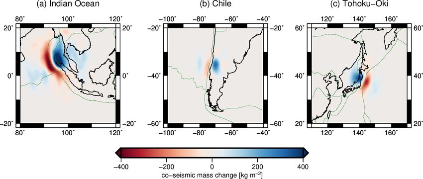
100                                                       A. Kvas et al.: GOCO06s – a satellite-only global gravity field model

1   Introduction                                                    ing observations over a longer time span allows us to derive
                                                                    a mean (static) gravity field. After the end of the mission in
Global models of Earth’s static gravity field are crucial           2017, the GRACE Follow-On mission has continued the ob-
for geophysical and geodetic applications. These include            servations since 2018 (Kornfeld et al., 2019; Landerer et al.,
oceanography (e.g., Knudsen et al., 2011; Rio et al., 2014;         2020), following the same design principle.
Johannessen et al., 2014; Bingham et al., 2014), tectonics             To increase the spatial resolution, tailored to the require-
(e.g., Johannessen et al., 2003; Ebbing et al., 2018), or es-       ments of geodetic, geophysical and oceanographic appli-
tablishing global reference and height systems (e.g., Rum-          cations, the Gravity field and steady-state Ocean Circula-
mel, 2013; Gerlach and Rummel, 2013). A special class of            tion Explorer (GOCE) mission (Battrick, 1999; Flobergha-
global gravity field models consists of the models derived          gen et al., 2011) was realized and launched in 2009. In
solely from satellite observations. In contrast to terrestrial      addition to SST-hl, a gradiometer served for the first time
observations – which are generally sparse and collected by          as a core instrument to measure the second derivatives of
various instruments in different quality levels and samplings       the Earth’s gravitational potential in gradiometer reference
– satellite observations typically cover the entire Earth’s sur-    frame (Rummel and Colombo, 1985; Rummel et al., 2002;
face. As the measurements are captured with the same sen-           Rummel et al., 2011b; Johannessen et al., 2003). Due to
sor platform, the global accuracy level of the observations is      the design of the instrument (Stummer et al., 2012; Siemes
much more consistent compared to terrestrial observations.          et al., 2012, 2019), only four out of the six derivatives of the
This also alleviates adequate stochastic modeling at the ob-        Marussi tensor could be measured with high precision (VXX ,
servation level (Ellmer, 2018; Schubert et al., 2019) to subse-     VXZ , VY Y and VZZ ). Due to the measurement of the second
quently provide uncertainty information for the derived grav-       derivatives, the spatial resolution can be increased at the cost
ity field.                                                          of more complex noise characteristics. Since the determina-
   The era of dedicated gravity field satellite missions (Rum-      tion of the long-wavelength signal is not accurate enough for
mel et al., 2002) provided a huge set of observations of            time-variable gravity inversion, the focus of GOCE is on the
the static as well as time-variable gravity field. The satel-       static gravity field. In the same fashion as for the other mis-
lite orbits are sensitive to the long wavelength of the grav-       sions, multiple expert groups perform gravity field recovery
ity field (e.g., Montenbruck and Gill, 2000; Rummel et al.,         with different processing strategies (e.g., Pail et al., 2011;
2002). They are either determined from ground by satellite          Farahani et al., 2013; Migliaccio et al., 2011; Brockmann
laser ranging (SLR) or from space via the tracking of a low-        et al., 2014; Schall et al., 2014; Yi, 2012).
Earth orbiter (LEO) with the satellites of the Global Posi-            Within typical processing workflows, mission (or tech-
tion System (GPS) constellation. The laser tracking of high-        nique) specific gravity field models are derived by technique-
flying SLR satellites is sensitive only for the longest wave-       specific experts and published as mission/technique-only
lengths but allows us to observe the temporal variations as         gravity field models. These models are published in terms
well (e.g., Maier et al., 2012; Sośnica et al., 2015; Bloßfeld     of a spherical harmonic expansion and reflect the state-of-
et al., 2018). The CHAllenging Minisatellite Payload satel-         the-art analysis. Nowadays, these models are more often
lite mission (CHAMP, Reigber et al., 1999) was the first ded-       equipped with a full covariance matrix, which reflects the
icated gravity field mission tracked by GPS. Since then mul-        error structure specific to the analysis and observation tech-
tiple other dedicated and non-dedicated satellites equipped         nique (e.g.,Brockmann et al., 2014; Bruinsma et al., 2014;
with GPS receivers have been used to derive static and tem-         Mayer-Gürr et al., 2018a; Kvas et al., 2019a).
poral gravity field models of the Earth (e.g., Bezděk et al.,         With a full covariance matrix in combination with a so-
2016; Lück et al., 2018; Teixeira da Encarnação et al., 2016)       lution vector, the original system of normal equations can
in this so-called satellite-to-satellite tracking in SST high–      be reconstructed. Together with additional meta-information,
low (SST-hl) configuration.                                         such as the number of observations and the weighted square
   Although SST-hl is sensitive to shorter wavelengths due to       sum of the observation vector, multiple gravity field solu-
the generally lower satellite altitude compared to SLR, the         tions can be used to derive combined gravity field models.
spatial resolution is still limited. With the Gravity Recov-        As long as the observations used are statistically indepen-
ery and Climate Experiment (GRACE) twin satellite mission           dent, the solution is the same as when starting from the raw
launched in 2002 (Tapley et al., 2004, 2019), inline satellite-     observations. Combining multiple observation principles and
to-satellite tracking (SST low–low, SST-ll) was established.        satellite missions (LEOs, GRACE, GOCE and SLR) has the
This then novel measurement principle relies on very precise        advantage that possible weaknesses of the individual contri-
measurements of inter-satellite distance variations between         butions can be compensated for. However, for a proper rela-
a leading and a trailing satellite in the same orbit. While         tive weighting, it is essential that the individual models used
GRACE is dedicated to observe temporal changes in Earth’s           provide a realistic error description in form of the covariance
gravitational field, typically in the form of monthly snapshots     matrix of the spherical harmonic coefficients. In the case of
(e.g., Rummel et al., 2002; Tapley et al., 2004; Mayer-Gürr,        satellite-only gravity field models, which are currently given
2006; Q. Chen et al., 2018; Beutler et al., 2010), accumulat-       to at most degree 300, SLR typically dominates the very long

Earth Syst. Sci. Data, 13, 99–118, 2021                                                https://doi.org/10.5194/essd-13-99-2021
A. Kvas et al.: GOCO06s – a satellite-only global gravity field model 101 wavelengths (degree 2 to 5), the medium wavelengths are GOCO satellite-only models are widely used and accepted mainly determined by GRACE (up to degree 130) and GOCE as state of the art by the community. The models published is the main contributor to the medium to short wavelengths so far (GOCO01s, GOCO02s, GOCO03s, and GOCO05s) (degree 130 to 300) (e.g., Pail et al., 2011; Maier et al., 2012; were used in a wide range of applications, for example, for Yi et al., 2013). global and local high-resolution models (e.g., Huang and Primary focus of combined models is the static grav- Véronneau, 2013; Pail et al., 2016, 2018; Klees et al., 2018; ity field (e.g., Pail et al., 2010; Farahani et al., 2013; Yi Slobbe et al., 2019), geophysical studies (e.g., Rummel et al., et al., 2013); nevertheless, some of the more recent mod- 2011a; Abrehdary et al., 2017; W. Chen et al., 2018), oceano- els also incorporate temporal variations, for example (piece- graphic studies (e.g., Farrell et al., 2012; Siegismund, 2013), wise) linear trends or annual oscillations (e.g., Rudenko or geodetic height unification (e.g., Vergos et al., 2018). et al., 2014). Since 2011, various models and approaches Within this contribution, the latest release – GOCO06S combining mainly GRACE and GOCE have been published. (Kvas et al., 2019b) – is presented. For that purpose, the Whereas Farahani et al. (2013) did a joint least-squares anal- data used to estimate the global satellite-only model are dis- ysis of GRACE and GOCE observations spending a lot of ef- cussed in Sect. 2. Section 3 covers the parametrization, which fort on the stochastic modeling of the observations, Yi et al. was used to describe the gravity field as well as its tempo- (2013) combined their self-computed GOCE normal equa- ral changes. Furthermore, the applied methods are discussed. tions with the publicly available ITG-Grace2010 model. The properties of the final estimate are discussed in Sect. 4 A specific and updated series of combined satellite-only and validated with state-of-the-art concepts. Section 6 sum- models is provided by the EIGEN-*S series which started as marizes the main characteristics of the model and presents a pure CHAMP-only model (Reigber et al., 2003) and turned some conclusions following from the analysis. to a GRACE, GOCE and SLR combination model in the lat- est EIGEN-6S release (Förste et al., 2016). These models are 2 Data sources and background models closely related to the GOCE solutions determined with the direct approach, which are already combination models (Bru- 2.1 Gravity field and steady-state Ocean Explorer insma et al., 2014, 2013). Basically, GRACE normal equa- (GOCE) tions processed by CNES/GRGS (Bruinsma et al., 2010) or GFZ (Dahle et al., 2019) are combined with GOCE normal The GOCO models make use of the normal equations of equations assembled with the so-called direct approach (Bru- the time-wise gravity field models (e.g., Pail et al., 2011; insma et al., 2014; Pail et al., 2011) and SLR normal equa- Brockmann et al., 2014). They are independent of any other tions. The combination is performed on the normal equation gravity field information and only contain measurements col- level. To counteract the non-perfect stochastic modeling in lected by GOCE. Furthermore, due to the use of an advanced the GRACE, GOCE and SLR analysis, the combination is stochastic model for the gravity gradients during the assem- performed only for certain manually chosen degree ranges, bly of the satellite gravity gradient (SGG) normal equations, which are selected according to the strengths of the individ- the formal errors are a realistic description of the uncertain- ual techniques. ties, which is beneficial for the combination procedure. This paper continues the global satellite-only models of Within GOCO06s, normal equations from the time-wise the GOCO*s series, which are produced by the Gravity RL06 model (GO_CONS_EGM_TIM_RL06, Brockmann Observation Combination (GOCO) consortium (http://www. et al., 2019; Brockmann et al., 2021) are used, which are goco.eu, last access: 20 January 2021). Since 2010, a se- based on SGG observations of the latest reprocessing cam- ries of satellite-only models (Pail et al., 2010) have been paign in 2019. A single unconstrained normal equation as- computed by the group, which is composed by experts on sembled from the VXX , VXZ , VY Y and VZZ gravity gradient SST-hl, GRACE, GOCE and SLR-based gravity field deter- observations up to spherical harmonic degree 300 enters the mination. The GOCO models combine the GRACE models computation of GOCO06s (see Sect. 3). produced by the Graz University of Technology (previously Due to the sensitivity of the gravity gradients and their ITG Bonn, now ITSG series, Mayer-Gürr et al., 2018b; Kvas spectral noise characteristics, normal equations are assem- et al., 2019a) with the time-wise GOCE normal equations bled only with respect to the static part of the Earth’s gravity (Brockmann et al., 2014), SST-hl normal equations of several field. To define a clear reference epoch and being consistent LEOs (Zehentner and Mayer-Gürr, 2016) and since the sec- with the GRACE processing, the time-variable gravity signal ond release GOCO02S SLR normal equations (Maier et al., was reduced from the along-track gravity gradient observa- 2012). Within the assembly of all the individual models used, tions in advance. For this purpose, the models as summarized a lot of effort is spent on the data-adaptive stochastic model- in Table 1 were used to refer the observations (and thus the ing of the observation error characteristics. Consequently, all right-hand side nSGG to the reference epoch 1 January 2010). input models come along with a realistic covariance matrix and are thus well suited as input for the applied combination procedure. https://doi.org/10.5194/essd-13-99-2021 Earth Syst. Sci. Data, 13, 99–118, 2021
102                                                           A. Kvas et al.: GOCO06s – a satellite-only global gravity field model

Table 1. Models used to reduce the temporal gravity changes.

             Force                                                    Model                            Reference
             Earth’s gravity field (annual oscillation and trend)     GOCO05s                          Mayer-Gürr et al. (2015)
             Non-tidal atmosphere and ocean variations
                                                                      AOD1B RL06                       Dobslaw et al. (2017)
             and atmospheric tides
             Astronomical tides (Moon, Sun, planets)                  JPL DE421                        Folkner et al. (2009)
             Solid Earth tides                                        IERS2010                         Petit and Luzum (2010)
             Ocean tides                                              FES2014b                         Carrere et al. (2015)
             Pole tides                                               IERS2010, linear mean pole       Petit and Luzum (2010)
             Ocean pole tides                                         Desai (2002), linear mean pole   Desai (2002)

  It enters the combination procedure (see Sect. 3) as a nor-              GRACE to the longer wavelengths of the spherical harmonic
mal equation system of the form                                            spectrum, it is the primary contributor to the temporal varia-
                                                                           tions.
NGOCE x̂ GOCE = nGOCE ,                                             (1)

where x̂ GOCE is the vector of unknown static spherical har-               2.3   Kinematic orbit of low-Earth orbit (LEO) satellites
monic coefficients, and NGOCE and nGOCE are the normal                     For GOCO06s, we made use of kinematic orbit posi-
equation coefficient matrix and right-hand side respectively.              tions from nine satellites. In addition to GRACE A/B (see
This system of normal equations is given in a predefined or-               Sect. 2.2), these include CHAMP, TerraSAR-X, TanDEM-X,
dering for the GOCE contribution (spherical harmonic de-                   GOCE and SWARM A+B+C. The kinematic orbit positions
grees 2 to 300). This single normal equation already con-                  were computed using precise point positioning following the
tains the stochastic models used in the time-wise process-                 approach of Zehentner and Mayer-Gürr (2016). The normal
ing (cf. Schubert et al., 2019), the relative weighting of                               (s)  (s)
                                                                           equations Nk , nk for gravity field determination were as-
the different gravity gradients and the different time peri-               sembled using the short-arc approach (Mayer-Gürr, 2006;
ods of observations. It is the same normal equation as used                Teixeira da Encarnação et al., 2020) in monthly batches
in GO_CONS_EGM_TIM_RL06, which is in the context of                        for each satellite s and epoch k. For CHAMP, GRACE,
a GOCE-only model combined with SST-hl data and con-                       TerraSAR-X, TanDEM-X and SWARM we set up the normal
strained (cf. Brockmann et al., 2021).                                     equations up to degree and order 120, while for GOCE, due
                                                                           to the lower orbit altitude and the subsequent higher sensitiv-
2.2   Gravity Recovery and Climate Experiment (GRACE)                      ity, the normal equations were assembled up to degree and or-
                                                                           der 150. For all LEO satellites except GRACE, only the static
The GRACE contribution to GOCO06s consists of a sub-                       gravity field was modeled. We made the decision to not in-
set of the normal equations of ITSG-Grace2018s (Mayer-                     clude secular and annual variations in the parameter set based
Gürr et al., 2018; Kvas et al., 2019a). Similarly to the                   on practical considerations. Even though SST-hl has skill in
GOCE normal equations, ITSG-Grace2018s features a full                     determining the time-variable gravity field, the expected con-
stochastic model of the inter-satellite range rates used and               tribution of the LEO orbits to the temporal constituents, with
hence provides realistic formal errors. The normal equa-                   the presence of GRACE inter-satellite-ranging observations
tions used incorporate GRACE data in the time span of                      and SLR, will be low. That results in a steep trade-off be-
April 2002 to August 2016, because at the time of the com-                 tween the increase in solution quality and the computational
putation the reprocessed observation data (GRACE, 2018)                    demands required to set up the additional parameters. Since
for the single-accelerometer months starting from Septem-                  we applied an appropriate stochastic model in the assembly
ber 2016 to June 2017 were not yet publicly available. The                 of the systems of normal equations, the relative weighting
normal equations feature a static part parametrized up to de-              between the satellites and epochs is already contained in the
gree/order 200 and secular and annual variations up to de-                 normal equations. Therefore, we only need to accumulate all
gree/order 120. The background models used in the process-                 satellites and months, as
ing of the GRACE data are consistent with the GOCE contri-                           XX (s)                  XX (s)
bution (see Kvas et al., 2019a, for details). The normal equa-             NLEO =            Nk , nLEO =            nk .               (3)
tions                                                                                 k   s                   k    s

NGRACE x̂ GRACE = nGRACE                                            (2)    The kinematic orbits provide gravity field information pri-
                                                                           marily to the lower (near-)sectorial coefficients of the spher-
are computed in monthly batches and then accumulated over                  ical harmonic spectrum, to which the GRACE inter-satellite
the observation time span. Due to the high sensitivity of                  range rates are less sensitive.

Earth Syst. Sci. Data, 13, 99–118, 2021                                                        https://doi.org/10.5194/essd-13-99-2021
A. Kvas et al.: GOCO06s – a satellite-only global gravity field model 103
2.4 Satellite laser ranging (SLR) Table 2. Relative weights of SLR satellites determined through
VCE.
To stabilize the long-wavelength part of the spectrum, we
added SLR observations to the combination. The observa- Satellite w(s) Satellite w(s)
tions used match the GRACE time span from April 2002 to
August 2016 and feature a total of 10 satellites, including LAGEOS 1 41.9 Etalon 1 1.0
LAGEOS 2 38.3 Etalon 2 1.6
LAGEOS 1/2, Ajisai, Stella, Starlette, LARES, LARETS,
Ajisai 3.2 LARES 1.1
Etalon 1/2 and BLITS. The SLR observations were pro- Stella 3.7 LARETS 3.2
cessed in weekly batches consisting of three 7 d arcs and Starlette 2.8 BLITS 3.0
one arc of variable length to complete the month, resulting
(s) (s) (s)
in systems of normal equations Nk x̂ k = nk up to d/o 60
for each satellite s. To obtain the normal equations for static,
3 Combination process
trend and annual oscillation from the weekly systems of nor-
mal equations, we first perform a parameter transformation. We combined the individual contributions from GOCE,
(s)
We express the weekly potential coefficients x k in terms of GRACE, kinematic LEO orbits, SLR and constraints on the
static, trend and annual oscillation as basis of normal equations using VCE. VCE is a widely
(s) (s) (s) used technique in geodesy for combining different observa-
x k = x static + x trend (tk − t0 ) + x (s)
cos cos(ω(tk − t0 ))+
(s)
tion groups (Koch and Kusche, 2002; Lemoine et al., 2013;
x sin sin(ω(tk − t0 )), (4) Meyer et al., 2019). The general idea is to determine the rel-
ative weights w∗ between heterogeneous observation types
or equivalently in matrix notation
within the same least-squares adjustment where the unknown
(s)
parameters, in our case the gravity field, are estimated. Typ-
xk = I I · (tk − t0 ) I · cos(ω(tk − t0 )) I · sin(ω(tk − t0 ))
| {z
:=F
}
ically, this is an iterative procedure where initial weights are
(s)
refined. The inverse of these weights, called variance factors,
x
static
(s) is the quotient of a residual square sum and the redundancy of
x trend
(s) . (5) the observation group. In the most general form this quotient
x cos
(s) is given as
x sin
Here, I is an identity matrix of appropriate dimension, t0 êT 6 −1 Vk 6 −1 ê
σk2 = , (8)
is the reference epoch of the combined gravity field and ω trace {(6 −1 − 6 −1 Ak N̄−1 ATk 6 −1 )Vk }
is the angular frequency corresponding to an oscillation of
where ê represents post-fit residuals, 6 = k σk2 Vk is the
P
365.25 d. Using this parameter substitution we can transform
the weekly systems of normal equations and accumulate over compound covariance matrix and Ak is the design matrix of
whole time span, the kth observation group. The iterative nature of VCE can be
(s)
X (s) (s)
X (s) seen in Eq. (8) where the compound covariance matrix com-
NSLR = FT Nk F, nSLR = FT nk . (6)
puted from the variance factors of the previous iteration is
k k
necessary to compute the new values. For observation groups
After the accumulation we determined the relative weight be- which are given as normal equations, so all satellite contri-
tween the individual SLR satellites s by variance component butions and also the Kaula constraint, this simplifies to
estimation (VCE). Since we processed all satellites consis-
tently, it is reasonable to assume that the formal errors are (l T Pl)k − 2nT x̂ + x̂ T Nk x̂
σk2 = . (9)
underestimated in the same fashion for all SLR targets, even n − trace {N̄−1 Nk } · σk−2
though no proper stochastic model for the SLR observation
was used in the processing. To determine the relative weights The general form presented in Eq. (8) comes into play when
w(s) of the satellites, we do not make use of the full system of we determine the weights of the regionally varying con-
normal equations but only use the static part up to degree and straints for the trend and annual signal (see Sect. 3.1). There
order 10. In Table 2, the determined relative weights can be we find that, for example, the variance factors for the trend
found. Note that these are specific to the processing applied constraint can be computed from
here.
Additionally, we applied a Kaula constraint to stabilize the x̂ Ttrend 6 −1 −1
Vk 6 x̂ trend
σk2 = . (10)
system of equations. The final normal equation matrix and trace {[6 −1 −1 −1 −1 −1
− 6 (N̄trend + 6 ) 6 ]Vk }
right-hand side used in the combination procedure are then
computed as the weighted sum of all satellites, Here, x̂ trend represents the estimated trend parameters, and
X X N̄trend is the accumulated system of normal equations of all
NSLR = w(s) N(s) , nSLR = w(s) n(s) . (7)
satellites. The determination of the relative weights w∗ = σ12
s s ∗
https://doi.org/10.5194/essd-13-99-2021 Earth Syst. Sci. Data, 13, 99–118, 2021104 A. Kvas et al.: GOCO06s – a satellite-only global gravity field model
is a key criterion for the overall solution quality. The GOCE,
GRACE and kinematic orbit contributions feature a proper
stochastic model of the observables used and therefore re-
alistic formal errors. This is a prerequisite for a proper de-
termination of relative weights using VCE (Meyer et al.,
2019). Consequently, the weights of these contributions re-
main close to 1 throughout the VCE iterations. The SLR
contribution used here lacks an adequate stochastic obser-
vation model, which results in formal accuracies that are too
optimistic. To counteract the high weights arising from this
mismodeling, the SLR system of normal equations was artifi-
cially down weighted by a factor of 10 in each iteration step.
The full, accumulated system of normal equations solved in
each iteration step is given by
N̄ = wGOCE NGOCE + wGRACE NGRACE + wLEO NLEO
+ wSLR NSLR + wKaula K + 6 −1
trend (w trend )
+ 6 −1
annual (w annual ), (11)
n̄ = wGOCE nGOCE + wGRACE nGRACE Figure 1. Structure of the combined normal equation coefficient
+ wLEO nLEO + wSLR nSLR . (12) matrix, with all contributions overlaid. The different parameter
groups for trend, annual and static potential coefficients are high-
It features all satellite contributions as well as constraints lighted and plotted to scale.
for certain parameters. In order to reduce the power in the
higher spherical harmonic degrees and specifically the polar
regions where the GOCE gradiometer observation provides the corresponding parameters. While the previous solution,
little to no information, the solution is zero-constrained us- GOCO05s, featured a simple Kaula constraint, GOCO06s
ing a Kaula-type signal model for degrees higher than 150. employs regionally varying prior information to account for
This Kaula regularization is represented by the matrix K. the greatly different signal levels in individual regions. Using
Furthermore, the co-estimated trend and annual oscillation a globally uniform signal model, which a Kaula-type regu-
are also zero-constrained with regionally varying regulariza- larization provides, damps the secular signal in, for example,
tion matrix 6 −1 −1
trend and 6 annual respectively. The vectors w trend Greenland while overestimating the expected signal level in
and wannual contain the weights for each modeled region (see the ocean. To avoid this undesired behavior, but still intro-
Sect. 3.1). duce as little prior information as possible, we developed a
The accumulation of the individual contributions in tailored regularization strategy.
Eq. (11) assumes that the individual normal equations are of As a first step, the globe was subdivided into regions
the same dimension. Since the maximum expansion degree with similar temporal behavior such as the ocean, Greenland,
differs between the techniques and not all contribute to the Antarctica, the Caspian Sea and the remaining land masses.
temporal variations, the systems of normal equations have to For each region i , a signal covariance matrix was derived
be zero-padded. The structure of the combined normal equa- by applying a window matrix Wi to a Kaula-type signal
tion coefficient matrix is depicted in Fig. 1. covariance model K. We construct the window matrix in the
We estimate 211 788 parameters in total with 90 597 to de- space domain by making use of spherical harmonic synthesis
scribe the static gravity field and 121 191 parameters for the and analysis. The general idea is to create an operator which
co-estimated temporal variations. Another 121 191 parame- propagates a vector of potential coefficients to source masses
ters representing co-seismic mass change caused by major on a grid (Wahr et al., 1998), applying a window function to
earthquakes (see Sect. 3.3) have been pre-eliminated. The this grid and then using quadrature (Sneeuw, 1994) to trans-
upper triangle of the (symmetric) normal equation coefficient form the windowed source masses back to potential coeffi-
matrix therefore requires 167 GB of memory. The published cients. All these operations are linear, so we can express the
system of normal equations only features the unconstrained window matrix as a matrix product,
static part with all temporal variations eliminated and re-
quires only 31 GB. Wi = AMi S. (13)
The diagonal matrix Mi is a binary window function con-
3.1 Regularization of co-estimated temporal variations
volved with a Gaussian kernel featuring a half width of
In order to properly decorrelate the co-estimated temporal 220 km (Jekeli, 1981) to mitigate ringing effects on region
variations from the long-term mean field, we constrained boundaries.
Earth Syst. Sci. Data, 13, 99–118, 2021 https://doi.org/10.5194/essd-13-99-2021A. Kvas et al.: GOCO06s – a satellite-only global gravity field model 105
Even though the observation contribution to the temporal
variations is band-limited to degree and order 120, as out-
lined in Sect. 2.2, the higher expansion degree of the sig-
nal covariance matrix does provide additional information.
Specifically, the transition between regions can be modeled
sharper thus enabling a better spatial separation. A similar
form of this approach, which combines band-limited obser-
vation information with high-resolution prior information,
can be found in Save et al. (2016). The resulting global, com-
pound covariance matrix
X X
6 = σi2 Wi KWTi = σi2 Vi (14)
i i
was then used to formulate a zero constraint for trend param-
eters y, with
0 = Iy + v, v ∼ N (0, 6 ), (15)
where I is a unit matrix of appropriate dimension. The for-
mulation of the compound covariance matrix in Eq. (14) im-
plies that the individual regions are treated as uncorrelated.
This has the side effect that 6 will be dense, even though
we use a Kaula-type signal covariance model.
For each region the unknown signal level σi was deter-
mined through VCE during the adjustment process. This
means that apart from the isotropic signal model shape, only
the geographic location of the region boundaries is intro-
duced as prior information. The same strategy was used to
regularize the annual oscillation; however, the globe was sub- Figure 2. Co-estimated secular variation of GOCO05s (a) and
divided into only two regions, namely continents and the GOCO06s (b) in equivalent water heights (EWH).
ocean. Furthermore, to conserve the phase of the oscillation,
a combined variance factor was estimated for both sine and
cosine coefficients. We compute the contribution of each component i ∈
The impact of this novel approach compared to the Kaula- {GOCE, GRACE, LEO, SLR} and the regularization by first
type regularization of the preceding GOCO satellite-only assembling the contribution or redundancy matrix
model on the estimated secular variations can be seen in Ri = N̄−1 Ni . (16)
Fig. 2. It is evident that the noise over the ocean is greatly
reduced in GOCO06s compared to its predecessor. In re- In Eq. (16), N̄ is the combined normal equation coefficient
gions where we have a large gradient in the signal level such matrix and Ni is the normal equation coefficient matrix of
as Greenland or the Antarctic Peninsula, we observe a bet- the ith component.
ter confinement of the signal within the land masses. This The main diagonal of Ri then gives an indication of how
means that with the new regularization strategy, less signal much each estimated parameter is informed by the respective
leaks from land into the ocean. But there are also limitations component i. Since we only look at estimated potential co-
to the employed approach. Looking at Greenland, a uniform efficients, it is convenient to depict the contribution to each
signal level for the region is not sufficient given the dramatic coefficient per degree and order in the coefficient triangle.
mass loss at the coasts. Still, there is a clear improvement Figure 3 shows the contribution to the static gravity field
visible in the new release, GOCO06s. of all contributing sources. We can clearly see the comple-
mentary nature of GRACE and GOCE, where the former is
the primary contributor to the long-wavelength part of the
3.2 Contribution of individual components
spectrum up to degree 130. GRACE also constrains and com-
When dealing with combined satellite models, the contribu- pensates for the polar gap of GOCE, which can be seen in the
tion of each component is of particular interest. It clearly higher contribution to the near-zonal coefficients up to degree
reveals the strengths and weaknesses of the different tech- 200. The GOCE SGG observations dominate degrees 130 to
niques in determining specific parts of the spherical harmonic 280. Between degrees 280 and 300, where we approach a
spectrum. signal-to-noise ratio of 1, the effect of regularization starts
https://doi.org/10.5194/essd-13-99-2021 Earth Syst. Sci. Data, 13, 99–118, 2021106 A. Kvas et al.: GOCO06s – a satellite-only global gravity field model
Figure 4. Contribution of (a) GRACE and (b) SLR to the estimated
trend. Note the different axis limits.
Figure 5. Contribution of (a) GRACE and (b) SLR to the estimated
annual oscillation. Note the different axis limits.
near-sectorials around degree 15. These findings are consis-
Figure 3. Individual contribution to the static part of the estimated tent with Bloßfeld et al. (2015).
potential coefficients for (a) GRACE, (b) GOCE SGG, (c) Kaula We find a similar picture when looking at the contribu-
regularization, (d) LEO orbits and (e) SLR. Note the different axis
tions for the estimated trend and annual oscillation shown in
limits for panels (d) and (e).
Figs. 4 and 5.
3.3 Estimation of co-seismic gravity changes
to play a role. LEO orbits primarily contribute to coefficients The simple parametrization of Earth’s gravity field with
up to degree 10 and near-sectorial coefficients up to the maxi- static, trend and annual signal basis functions cannot capture
mum degree of the involved system of normal equations. The instantaneous gravity changes caused by, for example, large
resonance orders of GRACE, which occur on multiples of 15 earthquakes. This mismodeling results in an apparent secu-
(Cheng and Ries, 2017), are clearly visible in the contribu- lar variation in the affected regions as the co-seismic grav-
tion plots. These parts of the spectrum are determined less ity change is mapped into the trend estimate. To avoid this
accurately by the inter-satellite ranging data of GRACE (Seo behavior, we estimate an additional step function in regions
et al., 2008) and are therefore compensated for by the other where co-seismic mass change is expected, thus improving
techniques (see, e.g., the higher contribution of GOCE in this the description of the temporal evolution of Earth’s gravity
order). field. The methodology is exemplified on the basis of a sin-
SLR primarily contributes to degree 2 and even zonal co- gle earthquake dividing the whole observation time span into
efficients up to degree 12, with a minor contribution to the two intervals i = {1, 2}, where interval i = 1 refers to obser-
Earth Syst. Sci. Data, 13, 99–118, 2021 https://doi.org/10.5194/essd-13-99-2021A. Kvas et al.: GOCO06s – a satellite-only global gravity field model 107
vations before the event and i = 2 to the observations cap- The estimated co-seismic mass changes can be seen in
tured after the event, respectively. But it can be generalized Fig. 6. We can clearly observe that the estimated signal is
to any number of intervals in a straightforward manner. For spatially confined; therefore, we retain the redundancy out-
each interval we assemble the observation equations side of the defined area. The advantages and limitations
regarding the estimation of the trend are best exemplified
l i = Ai x i + e i ei ∼ N (0, 6 i ), (17) by comparison with the GRACE monthly solution and the
previous GOCO05s release (not accounting for co-seismic
with l i being the observation vector, Ai the design matrix, x i
changes). Figure 7 shows the estimated trends for GOCO05s
the static gravity field parameters and ei the residual vector.
and GOCO06s (including the new co-estimated step) to-
We then form the blocked system of observation equations
gether with the time series of monthly solutions from ITSG-
for the whole observation time span
Grace2018 (Kvas et al., 2019a), evaluated close to the epi-
l1 A
x1 e center of the 2004 Indian Ocean earthquake, where we ob-
= 1 + 1 . (18) serve a large co-seismic mass change.
l2 A2 x 2 e2
We can clearly observe that adding the co-estimation of
The next step is to perform the parameter transformation co-seismic events greatly improves the accuracy of the secu-
lar variations. However, the monthly solutions show different
x1 I I z rates before and after the event, which can obviously not be
= , (19)
x2 I x modeled by just a uniform trend over the whole observation
time span. This is however a deliberate trade-off to retain re-
where I is an identity matrix of appropriate dimension, x
dundancy in the trend estimates and simple usability of the
is the static gravity field for the whole time span and z is
data set.
the correction for interval i = 1. Substituting Eq. (19) into
Eq. (18) yields
4 Results and evaluation
l1 A1 A1 z e
= + 1 . (20)
l2 A2 x e2
The complete published data set of GOCO06s consists of
Since both x and z are global representations of Earth’s grav- a static gravity field solution up to degree and order 300,
ity field, the functional model in Eq. (20) would result in a an unconstrained system of normal equations of the static
loss of redundancy in regions where no co-seismic change part for further combination, secular and annual gravity field
occurred. To counteract this overparametrization, we intro- variations up to degree and order 200, and co-seismic mass
duce the pseudo-observations changes for three major earthquakes. All components are
published in widely used data formats such as the ICGEM
0 = Wz + w w ∼ N (0, 6 w ), (21) format for potential coefficients (Barthelmes and Förste,
2011) and the SINEX format for normal equations (IERS,
where W is a window matrix covering Earth’s surface except
2006).
for the region where a co-seismic change is expected. After
The data product of primary interest for the community
combining the pseudo-observations with the transformed ob-
certainly is the estimated static gravity field together with its
servation equations in Eq. (20), the resulting system of nor-
uncertainty information represented by the system of normal
mal equations has the structure
equations. Therefore, we focus our evaluations and discus-
N1 + WT 6 −1
ẑ n1
sions on these components.
w W N1
= . (22)
N1 N1 + N2 x̂ n1 + n2 Figure 8 depicts degree amplitudes of differences of state-
of-the-art satellite-only gravity field models and XGM2016,
Increasing the weight of the constraint, that is, setting 6 w → a gravity field model which combines GOCO05s and ter-
0, which in practice is done by scaling with a number close to restrial data (Pail et al., 2016). This is the explanation for
zero, then allows a signal in ẑ only in regions within the pre- the small differences between XGM2016 and GOCO05s in
defined area. This retains the redundancy in points which are the low degrees where the terrestrial data do not significantly
not affected by the earthquake, thus not influencing the esti- contribute. Because of the GOCE orbit inclination of 96.7◦ ,
mate x̂ there. We applied this approach to model three ma- no data are collected directly above the poles. This polar gap
jor earthquakes during the GRACE life span, specifically, the has a distinct mapping to certain low-order coefficients of
2004 Indian Ocean earthquake (Han et al., 2006), the 2010 the gravity field (Sneeuw and van Gelderen, 1997). Conse-
Chile earthquake (Han et al., 2010) and the 2011 Tohoku-Oki quently, these coefficients are highly correlated and less ac-
earthquake (Panet et al., 2018). Since GRACE is the primary curately determined in GOCE-only models, such as GOCE
contributor to the estimated temporal variations at these spa- TIM6, where no other gravity field information is used. To
tial scales, the parameter transformation was considered only avoid these low-order coefficients dominating the degree am-
for the corresponding GRACE normal equations. plitudes and to ensure a consistent comparison, we excluded
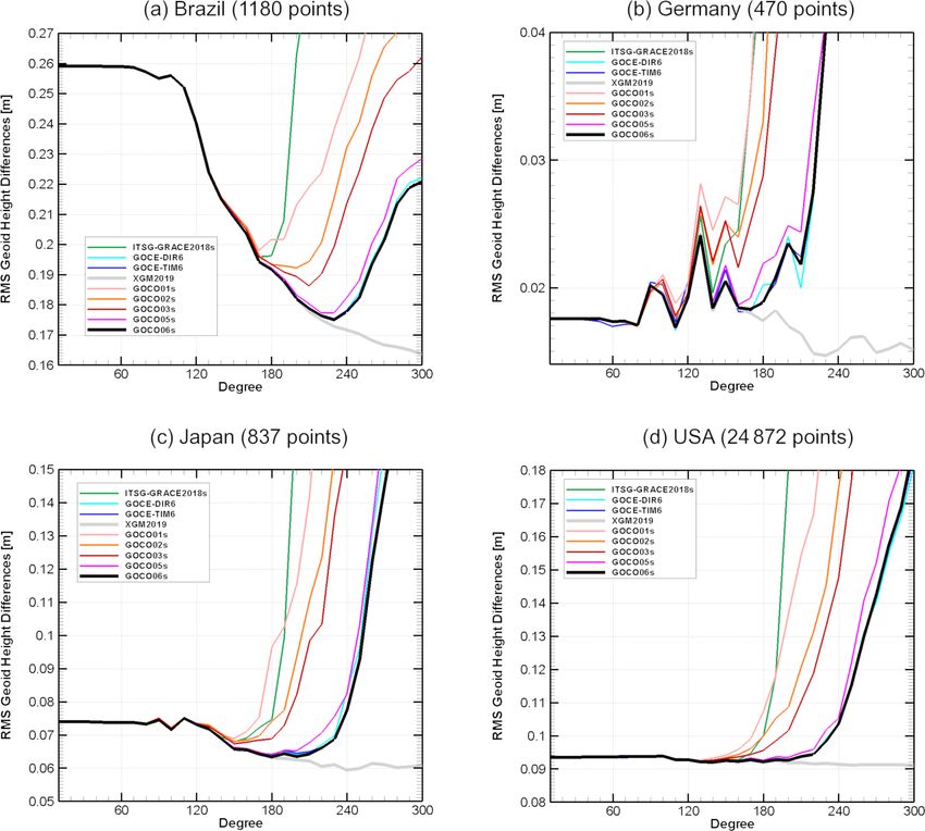
https://doi.org/10.5194/essd-13-99-2021 Earth Syst. Sci. Data, 13, 99–118, 2021108 A. Kvas et al.: GOCO06s – a satellite-only global gravity field model Figure 6. Estimated co-seismic mass change for all modeled earthquakes (230 km Gaussian filter applied). Figure 7. Comparison of estimated secular variation from GOCO05s, GOCO06s (including estimated co-seismic mass change) and filtered GRACE monthly solutions in terms of equivalent water height (EWH). The gravity field solutions were evaluated at 94.1◦ E, 3.1◦ N. the coefficients corresponding to a polar cap with 8◦ aperture to the final GOCO06s solution and shows the consistency of angle in all models, according to the rule of thumb given in formal and empirical errors. It further highlights the impor- Sneeuw and van Gelderen (1997). The differences between tance of stochastic modeling which enables this consistency. the compared models in degrees below 60 are, on the one The deviation of the combined solution from the GOCE SGG hand, explained by the respective reference epochs (for ex- contribution starting at degree 240 is explained by the Kaula ample, 1 January 2010 for GOCO06s and 1 September 2010 constraint applied to the combination. for GOCE DIR6) and, on the other hand, by the observation techniques used. GOCE TIM6 only relies on kinematic or- bit data and gradiometer observations, which do not reach 4.1 Comparison with GNSS leveling the superior accuracy of the GRACE inter-satellite ranging Over-land geoid heights (height anomalies or geoid undula- observations in this frequency band. In Fig. 8b, we can also tions) computed from global gravity models can be validated identify differences between the solutions starting from de- against independent geoid observations as they are deter- gree 150. Here, we can clearly distinguish between models mined by on ground GNSS leveling. By subtracting physical (GOCO06s, TIM6, DIR6) based on the latest reprocessing of heights determined by spirit leveling (orthometric or normal GOCE gradiometer data (version tag 0202) and models based heights) from ellipsoidal heights as they are observed with on the previous release (GOCO05s, EIGEN-GRGS RL04). GNSS, one can compute such independent geoid heights. Figure 9 shows the degree amplitudes of component-wise The challenge when comparing geoid heights derived from differences with respect to the combined solution of each satellite-only gravity field models to observed geoid heights component of GOCO06s. We excluded SLR here because the mainly is to eliminate the so-called omission error. This er- very ill posed system of normal equations can only be solved ror, which represents the higher-resolution geoid signal not up to degree 5–6 without additional information (Cheng observable by satellites due to the gravitational signal atten- et al., 2011). It nicely summarizes the major contributions uation at satellite altitude, causes the major part of the differ- Earth Syst. Sci. Data, 13, 99–118, 2021 https://doi.org/10.5194/essd-13-99-2021
A. Kvas et al.: GOCO06s – a satellite-only global gravity field model                                                             109

Figure 8. Difference degree amplitudes of various state-of-the-art satellite-only models compared to the combined model XGM2016 (polar
cap with 8◦ aperture angle excluded). Panel (a) shows the whole spherical harmonic spectrum covered by the models, while panel (b) only
shows degrees 150 to 300.

                                                                      high-resolution model of the gravity signal caused by the
                                                                      Earth’s topography such as ERTM2160 (Hirt et al., 2014) are
                                                                      used. The omission error computed from these models is sub-
                                                                      tracted from the observed geoid heights before they are com-
                                                                      pared to the satellite-only model geoid heights. Apart from
                                                                      this, a second systematic error might be present in physical
                                                                      heights observed by spirit leveling. Depending on the spirit-
                                                                      leveling technique and the carefulness of the observer, errors
                                                                      accumulate along the leveling lines, leading to artificial tilts
                                                                      (or other systematics) of the physical heights with respect to
                                                                      the reference equipotential surface, which is defined by the
                                                                      height system reference point in a country. Therefore, prior to
                                                                      analyzing differences between observed and global-model-
                                                                      derived geoid heights, a correction surface for the geoid dif-
                                                                      ferences shall be estimated and applied. This ensures that er-
                                                                      rors due to such tilts and due to offsets of regional height
                                                                      systems with respect to the global geoid are eliminated be-
                                                                      forehand. The computational procedure to compute and ana-
Figure 9. Difference degree amplitudes compared to GOCO06s            lyze geoid height differences between observed geoid heights
(solid lines) and corresponding formal errors (dashed lines) of the   and those determined from a global gravity field model is
individual GOCO06s components (polar cap with 8◦ aperture angle       described in detail in Gruber et al. (2011) and Gruber and
excluded). SLR is not shown because no stand-alone solution can       Willberg (2019).
be computed due to the ill-posed adjustment problem.                     For validating the GOCO06s model a number of global
                                                                      gravity field models and a number of GNSS-leveling data
                                                                      sets is applied. For gravity field models the previous satellite-
                                                                      only models of the GOCO series are used (GOCO01s,
ences leading to unrealistic quality estimates for the satellite-     GOCO02s, GOCO03s and GOCO05s). These models are
only gravity model. Therefore, the omission error needs to be         characterized by combining GRACE and GOCE satellite
estimated from other sources and taken into account prior to          data with an increasing number of observations and some
computing the differences. For this purpose, high-resolution          additional satellite data (see Sect. 1). In addition, an in-
gravity field models such as EGM2008 (Pavlis et al., 2012)            dependent SLR/GRACE/GOCE satellite-only combination
or XGM2019e (Zingerle et al., 2019, 2020) and an ultra-

https://doi.org/10.5194/essd-13-99-2021                                                   Earth Syst. Sci. Data, 13, 99–118, 2021
110 A. Kvas et al.: GOCO06s – a satellite-only global gravity field model model, namely GOCE-DIR6 (Förste et al., 2019), is used for sion error the worse the result of the differences is. This in- comparisons, which to a large extent is based on the same dicates that GOCE data can significantly improve the over- amount of SLR, GRACE and GOCE data as GOCO06s. In all performance of the global gravity field models in case order to identify the performance of pure GRACE and pure no high-quality ground data are available. In the other ar- GOCE models compared to the combined GOCO06s model, eas we consider here high-quality ground data were used in the ITSG-Grace2018s (Kvas et al., 2019a) model and the EGM2008, and therefore it performs very well when most GOCE-TIM6 (Brockmann et al., 2019; Brockmann et al., of the signal is computed from this model (i.e., for low trun- 2021) model are applied to the validation procedure. Finally, cation degrees). Looking to the different satellite-only solu- a model combining the GOCO06s satellite data with surface, tions one can identify the limit of a pure GRACE solution airborne and altimetric gravity data is used in order to iden- (ITSG-Grace2018s) as the rms of the differences starts to in- tify the signal content in higher degrees of the GOCO06s crease at lower degrees than for the other models. Including model. This is the XGM2019e high-resolution global grav- GOCE (and more GRACE) data significantly improves the ity field model (Zingerle et al., 2019, 2020). GNSS-leveling higher-resolution terms of the satellite-only models as it can data are available from many sources for many areas in the be seen from the series from GOCO01s to GOCO06s, where world. Typically, these data sets show different quality lev- the higher release number means more satellite information els, which strongly depend on the instruments, the measure- included. When comparing the satellite-only models to the ment procedure and the observer carefulness. In general, the combined XGM2019e model, the degree where they start to results for most of the comparisons show similar behavior diverge somehow represents the maximum signal content of but at different levels of accuracy. We have selected repre- the satellite-only models, or in other words up to what de- sentative data sets from different continents and of different gree and order such a model contains the full gravity field quality levels and validated the model-derived geoid heights signal. Depending on the area, we can identify that around against these data sets. Here we show the results for Brazil, degree 200 the models start to diverge. For Germany, where Germany, Japan and the United States (see Acknowledge- we probably have the best ground data set, the satellite con- ments). tribution is superior and may be up to degree 180. Regarding Figure 10 shows the results for the validation of the global the GOCO06s model we can state from these comparisons models against the independently observed geoid heights at that it is a state-of-the-art satellite-only model and that it per- GNSS-leveling points for the four selected countries. Before forms best together with the GOCE-DIR6 and GOCE-TIM6 drawing any conclusion from the results, the figure shall be models, which on the higher end of the spectrum are all based explained shortly. Each tested model was truncated at steps on the same complete GOCE data set. of degree 10 of the spherical harmonic series starting from degree and order 10 until 300. For each area the model geoid heights were computed up to the degree and order given on 4.2 Orbit residuals the x axis, and differences compared to the observed geoid heights were calculated. The omission error was computed To evaluate the long-wavelength part of GOCO06s, we an- separately from the EGM2008 and ERTM2160 models (see alyze orbit residuals between integrated dynamic orbits and above) starting from the truncation degree to highest possi- GPS-derived kinematic orbits of four LEO satellites of vari- ble resolution and subtracted from the geoid differences. Fi- ous altitudes and inclinations. The missions used with cor- nally, a planar correction surface was calculated for each area responding altitude and inclination are GOCE (≈ 250 km, for the geoid differences and subtracted. From the remain- 96.7◦ ), TerraSAR-X (Buckreuss et al., 2003, ≈ 515 km, ing differences the root-mean-square (rms) values shown on 98◦ ), Jason-2 (Neeck and Vaze, 2008, ≈ 1330 km, 66◦ ) and the y axis were computed. In general, the lowest level of the GRACE-B (≈ 450 km, 89◦ ). We realize that this is not a fully rms values is a good indicator of the quality of the GNSS- independent evaluation since GOCO06s contains kinematic leveling-derived geoid heights as one can assume that the orbit data from the LEO satellites considered here. However, global satellite-only models perform similarly over the whole since the overall contribution of the GPS positions to the globe. gravity field is very low (see Sect. 3.2), we argue that this Regarding this it becomes obvious that the German data approach still gives valid conclusions. Furthermore, we used set seems to be the best ground data set, while the Brazilian the kinematic GOCE and GRACE orbits of the Astronomical data set on average suffers from some inaccuracies, which Institute at Bern University (Bock et al., 2014; Meyer et al., are due to the size of the country and other geodetic infras- 2016) and not the in-house positions used in the gravity field tructure weaknesses. For Japan and the United States the rms recovery process. of differences is at a level of 7.5 and 9.5 cm respectively. The First, a dynamic orbit for each satellite is integrated based general shape of the curves is completely different for Brazil on a fixed set of geophysical models, where only the static and the other data sets under investigation. The reason be- gravity field is substituted. hind this is that the more information from the EGM2008 The models used can be found in Table 3. We included model (without GOCE data) is used for computing the omis- trend and annual gravity field variations from GRACE to Earth Syst. Sci. Data, 13, 99–118, 2021 https://doi.org/10.5194/essd-13-99-2021
A. Kvas et al.: GOCO06s – a satellite-only global gravity field model                                                            111

Figure 10. Root mean square of geoid height differences between global gravity models and independently observed geoid heights from
GNSS leveling. Global models are truncated with steps of 10◦ starting from degree and order 10 to degree and order 300. The omission
error is computed from the degree of truncation to degree and order 2190 from EGM2008 and from the ERTM2160 topographic gravity field
model for degrees above 2160.

make sure all compared gravity fields relate to the same ref-        ally superior to the model output, sensor-specific errors such
erence epoch.                                                        as bias and scale need to be considered. Consequently we
   Since satellites are not only affected by gravitational           model and estimate both bias and scale as well as empiri-
forces, but also non-conservative forces such as atmospheric         cal parameters for both accelerometers and model output to
drag, solar radiation pressure and Earth radiation pressure,         reduce the potential impact of mismodeling and sensor er-
both GOCE and GRACE are equipped with accelerometers                 rors on our evaluation. The values of these calibration pa-
which measure the impact of these forces. The other satel-           rameters are estimated together with the initial state when
lites (Jason-2, TerraSAR-X) do not feature such an instru-           the dynamic orbit is fitted to the kinematic satellite positions.
ment; therefore, we make use of models to compute the ef-            One constant bias for each axis and a single full-scale matrix
fect. Specifically, we model the impact of atmospheric drag          (Klinger and Mayer-Gürr, 2016) is estimated per each 1 d
(Bowman et al., 2008), Earth’s albedo (Knocke et al., 1988)          arc for all satellites. For Jason-2 and TerraSAR-X we addi-
and solar radiation pressure (Lemoine et al., 2013). Even            tionally estimate a once-per-revolution bias to further reduce
though the quality of accelerometer measurements is gener-           the impact of non-conservative forces. The metric we are us-

https://doi.org/10.5194/essd-13-99-2021                                                  Earth Syst. Sci. Data, 13, 99–118, 2021
112                                                       A. Kvas et al.: GOCO06s – a satellite-only global gravity field model

Table 3. Background models used in the dynamic orbit integration.

           Force                                  Model                                                 Maximum degree
           Earth’s static gravity field           static part of evaluated models                       200
           Annual/secular variations              estimated from CSR RL06 GRACE solutions               96
               of Earth’s gravity field               (DDK4 filter applied)
           Non-tidal ocean/atmosphere variation   AOD1B RL06                                            180
           Ocean tides                            FES2014b                                              180
           Astronomical tides                     IERS2010, JPL DE421                                   N/A
           Solid Earth tides                      IERS2010                                              4
           Atmospheric tides                      AOD1B RL06                                            180
           Pole tides                             IERS2010 (linear mean pole)                           c21 , s21
           Ocean pole tides                       Desai (2002, linear mean pole)                        220
           Relativistic corrections               IERS2010                                              –
           Non-conservative forces                measured if available, otherwise
                                                  JB2008 (drag), Knocke et al. (1988)/CERES (albedo),
                                                  Lemoine et al. (2013) (solar radiation pressure)      –

ing for the evaluation is the root mean square (rms) of the         GOCO06s and GOCO05s provide secular and annual vari-
orbit differences between the integrated dynamic orbit and          ations, while EIGEN-GRGS RL04 has secular, annual and
the purely GPS derived kinematic orbit positions. Epochs            semi-annual variations estimated for shorter intervals. We
where the difference exceeds 15 cm are treated as outliers          perform the evaluation for January 2020, which is well be-
and subsequently removed. We randomly selected 4 months             yond the GRACE measurement time span. This choice is de-
over the GOCE measurement time span (November 2009,                 liberate to assess the extrapolation capabilities of the com-
March 2010, October 2011 and March 2012).                           pared gravity fields. The computed rms values can be found
   We compare GOCO06s with its predecessor GOCO05s                  in Table 5.
and other recent static gravity field models (see Fig. 8) avail-       We can see that GOCO06s outperforms both its prede-
able on ICGEM (Ince et al., 2019). The results are summa-           cessor and EIGEN-GRGS RL04 while, unsurprisingly, the
rized in Table 4.                                                   GRACE-FO monthly solution performs best.
   From the computed rms values we can conclude that the
most recent combination models (GOCO06s and DIR6) per-              5   Data availability
form nearly equally well, with GOCO06s having a slight
edge. Furthermore, we can see that there is a quality jump          The primary model data consisting of potential coefficients
from the previous release, GOCO05s. The GOCE-only                   representing Earth’s static gravity field, together with sec-
model TIM6 performs the worst for all satellites, which high-       ular and annual variations, are available on ICGEM (Ince
lights the importance of GRACE for stabilizing the long to          et al., 2019). This data set is identified with the following
medium wavelengths and the polar gap. The overall larger            DOI: https://doi.org/10.5880/ICGEM.2019.002 (Kvas et al.,
rms values for TerraSAR-X and Jason-2 reflect the chal-             2019b) .
lenges in modeling non-conservative forces for these satel-            Supplementary material consisting of the full variance–
lites. Combined with the higher altitude, the contrast between      covariance matrix of the static potential coefficients and es-
the individual static gravity field solutions becomes very          timated co-seismic mass changes is available at https://ifg.
small. Still, we observe the same tendencies as for GOCE            tugraz.at/GOCO (last access: 11 June 2020).
and GRACE.
   Next to the validation of static gravity fields, orbit resid-
                                                                    6   Conclusions
uals are also very useful in evaluating the temporal con-
stituents of gravity field solutions. We gauge the qual-
                                                                    The satellite-only gravity field model GOCO06s provides a
ity of the co-estimated temporal constituents of GOCO06s
                                                                    consistent combination of spaceborne gravity observations
by integrating dynamic orbit arcs for GRACE Follow-On
                                                                    from a variety of satellite missions and measurement tech-
1 (GRACE-C). We compare GOCO06s to EIGEN-GRGS
                                                                    niques. Each component of the solution was processed using
RL04, a recent gravity field model which also features a
                                                                    state-of-the-art methodology which results in a clear increase
time-variable part; the previous solution, GOCO05s; and a
                                                                    in the solution quality compared to the preceding GOCO so-
GRACE-FO monthly solution. Instead of the trend and an-
                                                                    lutions and the individual input models. All contributing data
nual variation estimated from CSR RL06, we use the tem-
                                                                    sources were combined on the basis of full normal equations,
poral constituents of the gravity fields to be compared. Both
                                                                    with the individual weights being determined by VCE. The

Earth Syst. Sci. Data, 13, 99–118, 2021                                                https://doi.org/10.5194/essd-13-99-2021
You can also read