Global glacier volume projections under high-end climate change scenarios - The Cryosphere
←
→
Page content transcription
If your browser does not render page correctly, please read the page content below
The Cryosphere, 13, 325–350, 2019
https://doi.org/10.5194/tc-13-325-2019
© Author(s) 2019. This work is distributed under
the Creative Commons Attribution 4.0 License.

Global glacier volume projections under high-end
climate change scenarios
Sarah Shannon1,2 , Robin Smith3 , Andy Wiltshire4 , Tony Payne2 , Matthias Huss5,6 , Richard Betts1,4 , John Caesar4 ,
Aris Koutroulis7 , Darren Jones8 , and Stephan Harrison8
1 School of Geography, University of Exeter, The Queen’s Drive, Exeter, Devon, EX4 4QJ, UK
2 BristolGlaciology Centre, Department of Geographical Science, University Road, University of Bristol, BS8 1SS, UK
3 NCAS-Climate, Department of Meteorology, University of Reading, Reading, RG6 6BB, UK
4 Met Office, Fitzroy Road, Exeter, Devon, EX1 3PB, UK
5 Department of Geosciences, University of Fribourg, Fribourg, Switzerland
6 Laboratory of Hydraulics, Hydrology and Glaciology, ETH Zurich, Zurich, Switzerland
7 School of Environmental Engineering, Technical University of Crete, Akrotiri, 73100 Chania, Greece
8 University of Exeter, Penryn Campus, Treliever Road, Penryn, Cornwall, TR10 9FE, UK

Correspondence: Sarah Shannon (sarah.shannon@bristol.ac.uk)

Received: 15 February 2018 – Discussion started: 6 March 2018
Revised: 30 November 2018 – Accepted: 13 December 2018 – Published: 1 February 2019

Abstract. The Paris agreement aims to hold global warming          those on the peripheral of the Antarctic ice sheet. The uncer-
to well below 2 ◦ C and to pursue efforts to limit it to 1.5 ◦ C   tainty in the multi-model mean is rather small and caused
relative to the pre-industrial period. Recent estimates based      by the sensitivity of HadGEM3-A to the boundary condi-
on population growth and intended carbon emissions from            tions supplied by the CMIP5 models. The regions which
participant countries suggest global warming may exceed            lose more than 75 % of their initial volume by the end of
this ambitious target. Here we present glacier volume pro-         the century are Alaska, western Canada and the US, Iceland,
jections for the end of this century, under a range of high-end    Scandinavia, the Russian Arctic, central Europe, Caucasus,
climate change scenarios, defined as exceeding +2 ◦ C global       high-mountain Asia, low latitudes, southern Andes, and New
average warming relative to the pre-industrial period. Glacier     Zealand. The ensemble mean ice loss expressed in sea level
volume is modelled by developing an elevation-dependent            equivalent contribution is 215.2 ± 21.3 mm. The largest con-
mass balance model for the Joint UK Land Environment               tributors to sea level rise are Alaska (44.6 ± 1.1 mm), Arctic
Simulator (JULES). To do this, we modify JULES to include          Canada north and south (34.9 ± 3.0 mm), the Russian Arc-
glaciated and unglaciated surfaces that can exist at multi-        tic (33.3 ± 4.8 mm), Greenland (20.1 ± 4.4), high-mountain
ple heights within a single grid box. Present-day mass bal-        Asia (combined central Asia, South Asia east and west),
ance is calibrated by tuning albedo, wind speed, precipita-        (18.0 ± 0.8 mm), southern Andes (14.4 ± 0.1 mm), and Sval-
tion, and temperature lapse rates to obtain the best agreement     bard (17.0±4.6 mm). Including parametric uncertainty in the
with observed mass balance profiles. JULES is forced with          calibrated mass balance parameters gives an upper bound
an ensemble of six Coupled Model Intercomparison Project           global volume loss of 281.1 mm of sea level equivalent by
Phase 5 (CMIP5) models, which were downscaled using the            the end of the century. Such large ice losses will have in-
high-resolution HadGEM3-A atmosphere-only global cli-              evitable consequences for sea level rise and for water supply
mate model. The CMIP5 models use the RCP8.5 climate                in glacier-fed river systems.
change scenario and were selected on the criteria of passing
2 ◦ C global average warming during this century. The ensem-
ble mean volume loss at the end of the century plus or minus
1 standard deviation is −64 ± 5 % for all glaciers excluding

Published by Copernicus Publications on behalf of the European Geosciences Union.
326                                                                      S. Shannon et al.: Global glacier volume projections

1   Introduction                                                    resentative Concentration Pathways (RCP) RCP8.5 climate
                                                                    change scenario for high greenhouse gas emissions.
Glaciers act as natural reservoirs by storing water in the win-        The paper is organised as follows: in Sect. 2 we de-
ter and releasing it during dry periods. This is particularly vi-   scribe the glacier ice scheme implemented in JULES and
tal for seasonal water supply in large river systems in South       the procedure for initialising the model. Section 3 describes
Asia (Immerzeel and Bierkens, 2013; Lutz et al., 2014; Huss         how glacier mass balance is calibrated and validated for the
and Hock, 2018) and central Asia (Sorg et al., 2012) where          present day. Section 4 presents future glacier volume pro-
glacier melting contributes to streamflow and supplies fresh        jections, a comparison with other studies, and a discussion
water to millions of people downstream. Glaciers are also           on parametric uncertainty in the calibration procedure. Sec-
major contributors to sea level rise, despite their mass being      tion 5 discusses the results, model limitations, and areas for
much smaller than the Greenland and Antarctic ice sheets            future development. In Sect. 6, we summarise our findings
(Kaser et al., 2006; Meier et al., 2007; Gardner et al., 2013).     with some concluding remarks.
Since glaciers are expected to lose mass into the twenty-first
century (Radić et al., 2014; Giesen and Oerlemans, 2013;
Slangen et al., 2014; Huss and Hock, 2015), there is an ur-         2   Model description
gent need to understand how this will affect seasonal water
                                                                    JULES (described in detail by Best et al., 2011) characterises
supply and food security. To study this requires a fully inte-
                                                                    the land surface in terms of subgrid-scale tiles representing
grated impact model which includes the linkages and inter-
                                                                    natural vegetation, crops, urban areas, bare soil, lakes, and
actions among glacier mass balance, river runoff, irrigation,
                                                                    ice. Each grid box is comprised of fractions of these tiles
and crop production.
                                                                    with the total tile fraction summing to 1. The exception to
   The Joint UK Land Environment Simulator (JULES) (Best
                                                                    this is the ice tile, which cannot co-exist with other surface
et al., 2011) is an appropriate choice for this task because it
                                                                    types in a grid box. A grid box is either completely covered
models these processes, but it is currently missing a represen-
                                                                    in ice or not. All tiles can be assigned elevation offsets from
tation of glacier ice. JULES is the land surface component of
                                                                    the grid box mean, which is typically set to zero as a default.
the Met Office global climate model (GCM), which is used
                                                                       To simulate the mass balance of mountain glaciers more
for operational weather forecasting and climate modelling
                                                                    accurately we extend the tiling scheme to flexibly model
studies. JULES was originally developed to model vegetation
                                                                    the surface exchange in different elevation classes in each
dynamics and snow and soil hydrological processes within
                                                                    JULES grid box. We have added two new surface types,
the GCM but now has a crop model to simulate crop yield
                                                                    glaciated and unglaciated elevated tiles, to JULES (version
for wheat, soybean, maize, and rice (Osborne et al., 2014),
                                                                    4.7) to describe the areal extent and variation in height of
an irrigation demand scheme to extract water from ground
                                                                    glaciers in a grid box (Fig. 1). Each of these new types, at
and river stores, and two river routing schemes: Total Runoff
                                                                    each elevation, has its own bedrock subsurface with a fixed
Integrating Pathways (Oki et al., 1999) (TRIP) and the RFM
                                                                    heat capacity. These subsurfaces are impervious to water, and
kinematic wave model (Bell et al., 2007). The first objec-
                                                                    have no carbon content, so they have no interaction with the
tive of this study is to add a glacier ice scheme to JULES to
                                                                    complex hydrology or vegetation found in the rest of JULES.
contribute to the larger goal of developing a fully integrated
                                                                    Because glaciated and unglaciated elevated tiles have their
impact model.
                                                                    own separate bedrock subsurface they are not allowed to
   The second objective is to make projections of glacier
                                                                    share a grid box with any other tiles. For instance, grid boxes
volume changes under high-end climate change scenarios,
                                                                    cannot contain partial coverage of elevated glacier ice and
defined as exceeding 2 ◦ C global average warming relative
                                                                    vegetated tiles.
to the pre-industrial period (Gohar et al., 2017). The Paris
                                                                       JULES is modified to enable tile heights to be specified in
agreement aims to hold global warming to well below 2 ◦ C
                                                                    metres above sea level (m a.s.l.), as opposed to the default op-
and to pursue efforts to limit it to 1.5 ◦ C relative to the pre-
                                                                    tion, which is to specify heights as offsets from the grid box
industrial period; however, there is some evidence that this
                                                                    mean. This makes it easier to input glacier hypsometry into
target may be exceeded. Revised estimates of population
                                                                    the model and to compare the output to observations for par-
growth suggest there is only a 5 % chance of staying below
                                                                    ticular elevation bands. To implement this change, the grid
2 ◦ C and that the likely range of temperature increase will
                                                                    box mean elevation associated with the forcing data is read
be 2.0–4.9 ◦ C (Raftery et al., 2017). A global temperature
                                                                    in as an additional ancillary file. Downscaling of the climate
increase of 2.6–3.1 ◦ C has been estimated based on the in-
                                                                    data, described in Sect. 2.1, is calculated using the difference
tended carbon emissions submitted by the participant coun-
                                                                    between the elevation band (zband ) and the grid box mean
tries for 2020 (Rogelj et al., 2016). Therefore, in this study
                                                                    elevation (zgbm ).
we make end-of-the-century glacier volume projections, us-
ing a subset of downscaled Coupled Model Intercompari-              1z = zband − zgbm                                           (1)
son Project Phase 5 (CMIP5) models which pass 2 and 4 ◦ C
global average warming. The CMIP5 models use the Rep-

The Cryosphere, 13, 325–350, 2019                                                        www.the-cryosphere.net/13/325/2019/
S. Shannon et al.: Global glacier volume projections                                                                              327

Figure 1. Schematic of JULES surface types inside a single grid box. The new elevated glaciated and unglaciated tiles are shown on the
left-hand side. Note that elevated glaciated and unglaciated tiles are not allowed to share a grid box with the other tiles.

For the purposes of this study JULES is set up with a spa-
tial resolution of 0.5◦ and 46 elevation bands ranging from 0
to 9000 m in increments of 250 m. The horizontal resolution          SMBz,t = Sz,t − Sz,t−1                                       (2)
of 0.5◦ is used because it matches the forcing data used to          The scheme assumes that the snowpack can grow or shrink at
drive the model. The vertical resolution of 250 m was used           elevation bands depending on the mass balance, but that tile
based on computational cost. The vertical and horizontal res-        fraction (derived from the glacier area) is static with time.
olutions of the model can be modified for any setup.                 The ability to grow or shrink the snowpack at elevation lev-
   Each elevated glacier tile has a snowpack which can gain          els means that the model includes a simple elevation feed-
mass through accumulation and freezing of water and lose             back mechanism. If the snowpack shrinks to zero at an el-
mass through sublimation and melting. JULES has a full en-           evation band, then the terminus of the glacier moves to the
ergy balance multilevel snowpack scheme which splits the             next level above. Conversely, if the snowpack grows at an el-
snowpack into layers, each having a thickness, temperature,          evation band it just continues to grow and there is no process
density, grain size (used to determine albedo), and solid ice        to move the ice from higher elevations to lower elevations.
and liquid water contents. The initialisation of the snowpack        Typically, in an elevation feedback, when a glacier grows the
properties and the distribution of the glacier tiles as a func-      surface of the glacier will experience a cooler temperature;
tion of height are described in Sect. 2.3. Fresh snow accu-          however in this case, the snowpack surface experiences the
mulates at the surface of the snowpack at a characteristic low       temperature of the elevation band.
density and compacts towards the bottom of the snowpack
under the force of gravity. When rain falls on the snowpack,         2.1     Downscaling of climate forcing on elevations
water is percolated through the layers if the pore space is
sufficiently large, while any excess water contributes to the        Both glaciated and unglaciated elevated tiles are assigned
surface runoff. Liquid water below the melting temperature           heights in metres above sea level and the following adjust-
can refreeze. A full energy balance model is used to calculate       ments are made to the surface climate in grid boxes in which
the energy available for melting. If all the mass in a layer is      glaciers are present.
removed within a model time step then removal takes place
in the layer below. The temperature at each snowpack level is        2.1.1    Air temperature and specific humidity
calculated by solving a set of tridiagonal equations for heat
                                                                     Temperature is adjusted for elevation using a dry and moist
transfer with the surface boundary temperature set to the air
                                                                     adiabatic lapse rate depending on the dew point temperature.
temperature and the bottom boundary temperature set to the
                                                                     First the elevated temperature follows the dry adiabat:
subsurface temperature.
   A snowpack may exist on both glaciated and unglaciated            Tz = T0 − γdry 1z,                                           (3)
elevated tiles if there is accumulation of snow. The elevation-
dependent mass balance (SMBz,t ) is calculated as the change         where T0 is the surface temperature, γdry is the dry adiabatic
in the snowpack mass (S) between successive time steps.              temperature lapse rate (◦ C m−1 ), and 1z is the height differ-
                                                                     ence between tile elevation and the grid box mean elevation
                                                                     associated with the forcing data.

www.the-cryosphere.net/13/325/2019/                                                           The Cryosphere, 13, 325–350, 2019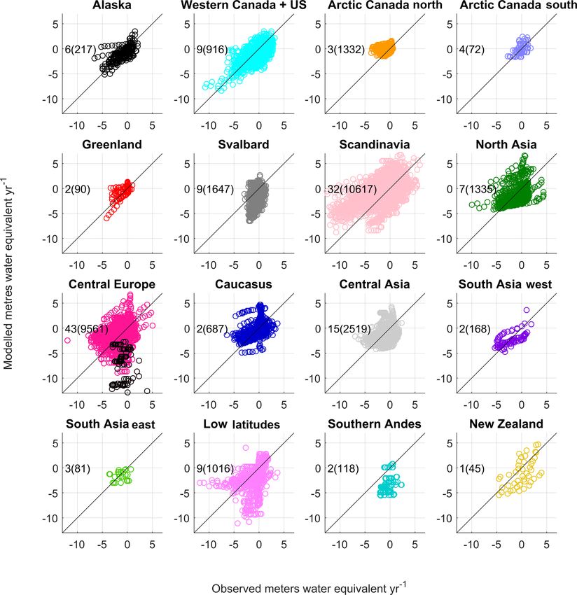
328                                                                       S. Shannon et al.: Global glacier volume projections

  If Tz is less than the dew point temperature Tdew then the      An additional correction is made to ensure that the grid box
temperature adjustment follows the moist adiabat. A moist         mean downward longwave radiation is preserved:
adiabatic lapse rate is calculated using the surface specific                       n
                                                                                    X                               LW↓z
humidity from the forcing data.                                   LW↓z = LW↓z −           LW↓z · frac (z)                           , (11)
                                                                                                            z
                                                                                                            P
                                                                                  z=1                           LW↓z · frac (z)
                g(1+lc·q0 )                                                                                 i=1
                r·Tv (1−q0 )
γmoist =                                                 (4)    where frac is the tile fraction.
               Cp +lc·2·q0 ·R
               r·Tv 2(1−q0 )
                                                                  2.1.3     Precipitation
q0 is the surface specific humidity, lc is the latent heat of
fusion of water at 0 ◦ C (2.501 × 10⁶ J kg−1 ), g is the accel-   To account for orographic precipitation, large-scale and con-
eration due to gravity (9.8 m s−2 ), r is the gas constant for    vective rainfall and snowfall are adjusted for elevation using
dry air (287.05 kg K−1 ), R is the ratio of molecular weights     an annual mean precipitation gradient (%/100 m):
of water and dry air (0.62198), and Tv (K) is the virtual dew
                                                                  Pz = P0 + P0 γprecip (z − z0 ) ,                                    (12)
point temperature.
                                                                where P0 is the surface precipitation, γprecip is the precipita-
                 1
Tv = Tdew (1 +      − 1.0 q0 )                              (5)   tion gradient, and z0 is the grid box mean elevation. Rainfall
                 R                                                is also converted to snowfall when the elevated air tempera-
                                                                  ture Tz is less than the melting temperature (0 ◦ C). The ad-
The height at which the air becomes saturated z is
                                                                  justed precipitation fields are input into the snowpack scheme
      T0 − Tdew                                                   and the hydrology subroutine. When calibrating the present-
z=              .                                          (6)    day mass balance, we needed to lapse rate correct the precip-
         γdry
                                                                  itation to obtain sufficient accumulation in the mass balance
The elevated temperature following the moist adiabat is then      compared to observations. The consequence of this is that
                                                                  the grid box mean precipitation is no longer conserved. We
Tz = Tdew − (1z − z) γmoist .                              (7)    tested scaling the precipitation in a way that conserves the
                                                                  grid box mean by reducing the precipitation near the surface
Additionally, when Tz < Tdew , the specific humidity is ad-       and increasing it at height, but this did not yield enough pre-
justed for height. The adjustment is made using the elevated      cipitation to obtain a good agreement with the mass balance
air temperature and surface pressure from the forcing data us-    observations. If the model is being used to simulate river dis-
ing a lookup table based on the Goff–Gratch formula (Bakan        charge in glaciated catchments, then the precipitation lapse
and Hinzpeter, 1987). The adjusted humidity is then used in       rate could be used as a parameter to calibrate the discharge.
the surface exchange calculation.
                                                                  2.1.4     Wind speed
2.1.2   Longwave radiation
                                                                  A component of the energy available to melt ice comes from
Downward longwave radiation is adjusted by assuming               the sensible heat flux, which is related to the temperature dif-
the atmosphere behaves as a black body using Stefan–              ference between the surface and the elevation level and the
Boltzmann’s law. The radiative air temperature at the surface     wind speed. Glaciers often have katabatic (downslope) winds
Trad,0 is calculated using the downward longwave radiation        which enhance the sensible heat flux and increase melting
provided by the forcing data LW↓z0                                (Oerlemans and Grisogono, 2002). It is important to repre-
                      1                                         sent the effects of katabatic winds on the mass balance when
               LW↓z0      4                                       trying to model glacier melt, particularly at lower elevations
Trad,0 =                       ,                           (8)
                 σ                                                where the katabatic wind speed is highest.
                                                                     To explicitly model katabatic winds would require knowl-
where σ is the Stefan–Boltzmann constant (5.67 ×                  edge of the grid box mean slope at elevation bands, so instead
10−8 W m−2 K−4 ). The radiative temperature at height is          a simple scaling of the surface wind speed is used to rep-
then adjusted:                                                    resent katabatic winds. Over glaciated grid boxes the wind
                                                                  speed is
Trad,z = Trad,0 + Tz − T0 ,                                (9)
                                                                  uz = u0 γwind ,                                                     (13)
where T0 is the grid box mean temperature from the forcing
data and Tz is the elevated air temperature. This is used to      where γwind is a wind speed scale factor and u0 is the surface
calculate the downward longwave radiation LW↓z at height          wind speed. The simple scaling increases the wind speed rel-
                                                                  ative to the surface forcing data and assumes that the scaling
           4                                                      is constant for all heights.
LW↓z = σ Trad,z .                                         (10)

The Cryosphere, 13, 325–350, 2019                                                         www.the-cryosphere.net/13/325/2019/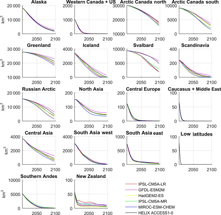
S. Shannon et al.: Global glacier volume projections                                                                                         329

   Although our approach is rather crude, we found that scal-                   2.3     Initialisation
ing the wind speed was necessary to obtain reasonable val-
ues for the sensible heat flux. This is seen when we compare                    The model requires initial conditions for (1) the snowpack
the modelled energy balance components to observations                          properties and (2) glaciated and unglaciated elevated tile
from the Pasterze glacier in the Alps (Greuell and Smeets,                      fractions within a grid box. The location of glacier grid
2001). The measurements consist of incoming and outgo-                          points, the initial tile fraction, and the present-day ice mass
ing short- and longwave radiation, albedo, temperature, wind                    are set using data from the Randolph Glacier Inventory ver-
speed, and roughness length at five heights between 2205 and                    sion 6 (RGI6) (RGI Consortium, 2017). This dataset contains
3325 m a.s.l. on the glacier. Table S6 in the Supplement lists                  information on glacier hypsometry and is intended to cap-
the observed and modelled energy balance components and                         ture the state of the world’s glaciers at the beginning of the
meteorological data, for experiments with and without wind                      twenty-first century. A new feature of the RGI6 is 0.5◦ grid-
speed scaling. The comparison shows that JULES underesti-                       ded glacier volume and area datasets, produced at 50 m ele-
mates the sensible heat flux by at least 1 order of magnitude                   vation bands. Volume was constructed for individual glaciers
and the modelled wind speed is 4 times lower than the ob-                       using an inversion technique to estimate ice thickness created
servations. When we increase the wind speed to match the                        using glacier outlines, a digital elevation model, and a tech-
observations there is a better agreement with the observed                      nique based on the principles of ice flow mechanics (Farinotti
sensible heat flux. The surface exchange coefficient, which                     et al., 2009; Huss and Farinotti, 2012). The area and vol-
is used to calculate the sensible heat flux, is a function of the               ume of individual glaciers have been aggregated onto 0.5◦
wind speed in the model.                                                        grid boxes. We bin the 50 m area and volume into elevations
                                                                                bands varying from 0 to 9000 m in increments of 250 m to
2.2    Glacier ice albedo scheme                                                match the elevation bands prescribed in JULES.

The existing spectral albedo scheme in JULES simulates the                      2.3.1    Initial tile fraction
darkening of fresh snow as it undergoes the process of aging
(Warren and Wiscombe, 1980). In this scheme the change in                       The elevated glaciated fraction is
albedo as snow ages is related to the growth of the snow grain                                   RGI_area(n)
size, which is a function of the snowpack temperature. The                      fracice(n) =                   ,                             (15)
                                                                                               gridbox_area(n)
snow aging scheme does not reproduce the low albedo val-
ues typically observed on glacier ice; therefore a new albedo                   where RGI_area is the area (km2 ) at height from the RGI6,
scheme is used. The new scheme is a density-dependent pa-                       n is the tile elevation, and gridbox_area (km2 ) is the area
rameterisation which was developed for implementation in                        of the grid box. In this configuration of the model, any area
the Surface Mass Balance and Related Sub-surface processes                      that is not glaciated is set to a single unglaciated tile fraction
(SOMARS) model (Greuell and Konzelmann, 1994). The                              (fracrock ) with a grid box mean elevation. It is possible to
scheme linearly scales the albedo from the value of fresh                       have an unglaciated tile fraction at every elevation band, but
snow to the value of ice, based on the density of the snowpack                  since the glaciated tile fractions do not grow or shrink, we re-
surface. The new scheme is used when the surface density of                     duce our computation cost by simply putting any unglaciated
the top 10 cm of the snowpack (ρsurface ) is greater than the                   area into a single tile fraction.
firn density (550 kg m−3 ) and the original snow aging scheme
                                                                                                 n=nBands
is used when (ρsurface ) is less than the firn density.                         fracrock = 1 −
                                                                                                   X
                                                                                                            fracice (n)                      (16)
                                                                                                 n=1
                                   αλ,snow − αλ,ice
αλ = αλ,ice + (ρsurface − ρice )                          (14)                  nBands = 37 is the number of elevation bands.
                                     ρsnow − ρice

αλ,snow is the maximum albedo of fresh snow, αλ,ice is the                      2.3.2    Initial snowpack properties
albedo of melting ice, ρsnow is the density of fresh snow
(250 kg m−3 ), and ρice is the density of ice (917 kg m−3 ).                    The snowpack is divided into 10 levels in which the top nine
The albedo scaling is calculated separately in two radiation                    levels consist of 5 m of firn snow with depths of 0.05, 0.1,
bands: visible (VIS) wavelengths λ = 0.3–0.7 µm and near-                       0.15, 0.2, 0.25, 0.5, 0.75, 1, and 2 m and the bottom level has
infrared (NIR) wavelengths λ = 0.7–5.0 µm. The parameters,                      a variable depth. For each snowpack level the following prop-
αvis,ice , αvis,snow , αnir,ice , αnir,snow , γtemp , γprecip , and γwind are   erties must be set: density (kg m−3 ), ice content (kg m−2 ),
tuned to obtain the best agreement between simulated and                        liquid water content (kg m−2 ), grain size (µm), and tempera-
observed surface mass balance profiles for the present day                      ture (K). We assume there is no liquid content in the snow-
(see Sect. 3).                                                                  pack by setting this to zero. The density at each level is lin-
                                                                                early scaled with depth, between the value for fresh snow at
                                                                                the surface (250 kg m−3 ) and the value for ice at the bottom
                                                                                level (917 kg m−3 ).

www.the-cryosphere.net/13/325/2019/                                                                         The Cryosphere, 13, 325–350, 2019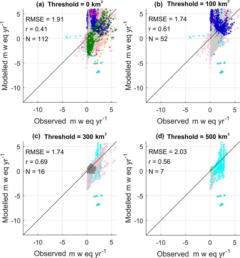
330                                                                       S. Shannon et al.: Global glacier volume projections

   For the future simulations the thickness and ice mass at          orographic precipitation gradient (γprecip ), temperature lapse
the bottom of the snowpack come from thickness and volume            rate (γtemp ), and wind speed scaling factor (γwind ).
data in the RGI6. The data are based on thickness inversion             Random parameter combinations are selected using Latin
calculations from Huss and Farinotti (2012) for individual           hypercube sampling (McKay et al., 1979) among plausible
glaciers which are consolidated onto 0.5◦ grid boxes. The ice        ranges which have been derived from various sources out-
mass is calculated from the RGI6 volume assuming an ice              lined below. This technique randomly selects parameter val-
density of 917 kg m−3 . For the other layers the ice mass is         ues; however, reflectance in the VIS wavelength is always
calculated by multiplying the density by the layer thickness,        higher than in the NIR. To ensure the random sampling does
which is prescribed above. For the calibration period, the ice       not select NIR albedo values that are higher or unrealistically
mass at the start of the run (1979) is unknown. In the absence       close to the VIS albedo values, we calculate the ratio of VIS
of any information about this, a constant depth of 1000 m            to NIR albedo using values compiled by Roesch et al. (2002).
is used, which is selected to ensure that the snowpack never         The ratio VIS / NIR is calculated as 1.2 so any albedo values
completely depletes over the calibration period. This consists       that exceed this ratio are excluded from the analysis. This
of 995 m of ice at the bottom level of the snowpack and 5 m          reduces the sample size from 1000 to 198 parameter sets.
of firn in the layers above. The ice content of the bottom level        In the VIS wavelength the fresh snow albedo is tuned be-
is the depth (995 m) multiplied by the density of ice.               tween 0.99 and 0.7 for which an upper bound value comes
   The snow grain size used to calculate spectral albedo (see        from observations of very clean snow with few impurities in
Sect. 2.2) is linearly scaled with depth and varies between          the Antarctic (Hudson et al., 2006). The lower bound rep-
50 µm at the surface for fresh snow and 2000 µm at the base          resents contaminated fresh snow and comes from taking ap-
for ice. The snowpack temperature profile is calculated by           proximate values from a study based on laboratory experi-
spinning the model up for 10 years for the calibration pe-           ments of snow, with a large grain size (110 µm) containing
riod and 1 year for the future simulations. The temperature          1680 parts per billion of black carbon (Hadley and Kirch-
at the top layer of the snowpack is set to the January mean          stetter, 2012). VIS snow albedos of approximately 0.7 have
temperature and the bottom layer and subsurface tempera-             also been observed on glaciers with black carbon and min-
ture are set to the annual mean temperature. For the calibra-        eral dust contaminants in the Tibetan Plateau (Zhang et al.,
tion period the monthly and annual temperature comes from            2017). In the NIR wavelength the fresh snow albedo is tuned
the last year of the spin-up. Setting the snowpack tempera-          between 0.85 and 0.5 for which the upper bound comes from
ture this way gives a profile of warming towards the bottom          spectral albedo observations made in Antarctica (Reijmer et
of the snowpack representative of geothermal warming from            al., 2001). We use a very low minimum albedo for ice in the
the underlying soil. The initial temperature of the bedrock          VIS and NIR wavelengths (0.1), in order to capture the low
before the spin-up is set to 0 ◦ C but this adjusts to the climate   reflectance of melting ice.
as the model spins up. We use these prescribed snowpack                 The temperature lapse rate is tuned between values of 4.0
properties as the initial state for the calibration and future       and 10 ◦ C km−1 for which the upper limit is determined from
runs.                                                                physically realistic bounds and the lower limit is from obser-
                                                                     vations based at glaciers in the Alps (Singh, 2001). The tem-
                                                                     perature lapse rate in JULES is constant throughout the year
3     Mass balance calibration and validation                        and assumes that temperature always decreases with height.
                                                                        The wind speed scaling factor γwind is tuned within the
3.1    Model calibration                                             range of 1–4 to account for an increase in wind speed with
                                                                     height and for the presence of katabatic winds. The upper
Elevation-dependent mass balance is calibrated for the               bound is estimated using wind observations made along the
present day by tuning seven model parameters and compar-             profile of the Pasterze glacier in the Alps during a field cam-
ing the output to elevation-band specific mass balance obser-        paign (Greuell and Smeets, 2001). Table S6 in the Supple-
vations from the WGMS (2017). Calibrating mass balance               ment contains the wind speed observations on the Pasterze
against in situ observations is a technique which has been           glacier. The maximum observed wind speed was 4.6 m s−1
used by other glacier modelling studies (Radić and Hock,            (at 2420 m a.s.l.) while the WATCH–ERA Interim dataset
2011; Giesen and Oerlemans, 2013; Marzeion et al., 2012).            (WFDEI) (Weedon et al., 2014) surface wind speed for the
For the calibration, annual elevation-band mass balance ob-          same time period was 1.1 m s−1 , indicating a scaling factor
servations are used because there are data available for 16          of approximately 4.
of the 18 RGI6 regions. For validation, winter and summer               The orographic precipitation gradient γprecip is tuned be-
elevation-band mass balance is used because there are fewer          tween 5 and 25 % per 100 m. This parameter is poorly con-
data available.                                                      strained by observations; therefore a large tuneable range
   The tuneable parameters for mass balance are VIS snow             is sampled. Tawde et al. (2016) estimated a precipitation
albedo (αvis,snow ), VIS melting ice albedo (αvis,ice ), NIR         gradient of 19 % per 100 m for 12 glaciers in the western
snow albedo (αnir,snow ), NIR melting ice albedo (αnir,ice ),        Himalayas using a combination of remote sensing and in

The Cryosphere, 13, 325–350, 2019                                                         www.the-cryosphere.net/13/325/2019/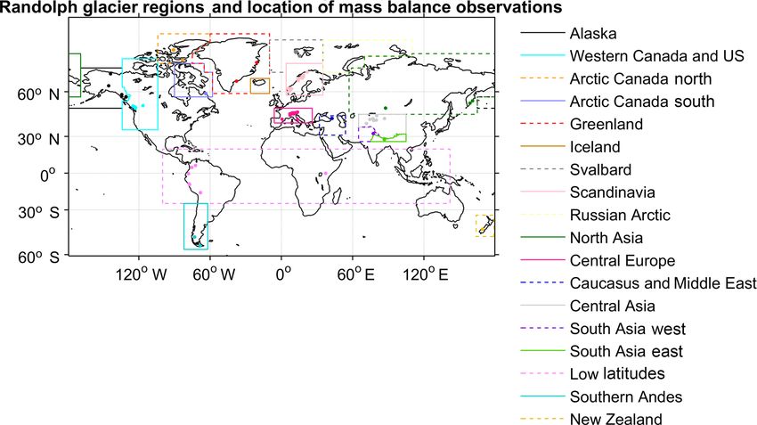
S. Shannon et al.: Global glacier volume projections                                                                               331

Table 1. Tuneable parameters for mass balance calculation and their ranges from the literature.

                               Parameter                            Range of values    Symbol      Units
                               Fresh snow albedo (VIS)                     0.99–0.7    αvis,snow   –
                               Fresh snow albedo (NIR)                     0.85–0.5    αnir snow   –
                               Ice albedo (VIS)                             0.7–0.1    αvis,ice    –
                               Ice albedo (NIR)                             0.6–0.1    αnir,ice    –
                               Temperature lapse rate                         4–9.8    γtemp       K km−1
                               Orographic precipitation gradient               5–25    γprecip     %/100 m
                               Wind speed scale factor                          1–4    γwind       –

situ meteorological observations of precipitation. Observa-             region, which has a large RMSE (3.02 m w.e. yr−1 ). This re-
tions show that the precipitation gradient can be as high               gion contains relatively small tropical glaciers in Colombia,
as 25 % per 100 m for glaciers in Svalbard (Bruland and                 Peru, Ecuador, Bolivia, and Kenya. Marzeion et al. (2012)
Hagen, 2002) while glacier–hydrological modelling studies               found a poor correlation with observations in the low-latitude
have used much smaller values of 4.3 % per 100 m (Sorg                  region when they calibrated their glacier model using Cli-
et al., 2014) and 3 % per 100 m (Marzeion et al. (2012).                matic Research Unit (CRU) data (Mitchell and Jones, 2005).
The tuneable parameters and their minimum and maximum                   They attributed that to the fact that sublimation was not in-
ranges are listed in Table 1.                                           cluded in their model, a process which is important for the
   The model is forced with daily surface pressure, air tem-            mass balance of tropical glaciers. Our mass balance model
perature, downward longwave and shortwave surface radi-                 includes sublimation, so it is possible the WFDEI data over
ation, specific humidity, rainfall, snowfall, and wind speed            tropical glaciers are too warm. The WFDEI data are based
from the WFDEI dataset (Weedon et al., 2014). To reduce                 on the ERA-Interim reanalysis in which air temperature has
the computation time, only grid points at which glacier ice is          been constrained using CRU data. The CRU data comprise
present are modelled. An ensemble of 198 calibration exper-             temperature observations which are sparse in regions where
iments are run. For each simulation the model is spun up for            tropical glaciers are located. Furthermore, the quality of the
10 years and the elevation-dependent mass balance is com-               WFDEI data will depend on the performance of the under-
pared to observations at 149 field sites over the years 1979–           lying ECMWF model. In central Europe some of the poor
2014.                                                                   correlations with observations are caused by the Maladeta
   The elevation-dependent mass balance observations come               glacier in the Pyrenees (Fig. 3), which is a small glacier with
from stake measurements taken every year at different                   an area of 0.52 km2 (WGMS, 2017). When this glacier is ex-
heights along the glaciers. Many of the mass balance obser-             cluded from the analysis the correlation coefficient increases
vations in the World Glacier Monitoring Service (WGMS,                  from 0.26 to 0.35 and the RMSE decreases from 2.03 to
2017) are supplied without observational dates. In this case,           1.73 m of water equivalent per year.
we assume the mass balance year starts on 1 October and
ends on 30 September with the summer commencing on                      3.2    Model validation
1 May. Dates in the Southern Hemisphere are shifted by 6
months. The observations are grouped according to standard-             The calibrated mass balance is validated against summer
ised regions defined by the RGI6 (Fig. 2). The best regional            and winter elevation-band specific mass balance for each
parameter sets are identified by finding the minimum root-              region where data are available (Fig. 4). For all regions,
mean-square error between the modelled mass balance and                 except Scandinavia in the summer, negative Nash–Sutcliffe
the observations.                                                       numbers are calculated for winter and summer elevation-
   Figure 3 shows the modelled mass balance profiles plot-              dependent mass balance (Table 4). The negative numbers
ted against the observations using the best parameter set for           arise because the bias in the model is larger than the variance
each region. The best regional parameter sets are listed in             of the observations. There are negative biases for nearly all
Table 2 and the root-mean-square error, correlation coeffi-             regions, implying that melting is overestimated in the sum-
cient, Nash–Sutcliffe efficiency coefficient, and mean bias             mer and accumulation is underestimated in the winter. This
are listed in Table 3. Nine out of the 16 regions have a                means that future projections of volume loss presented in
negative bias in the annual mass balance. Notably Svalbard,             Sect. 4.2 might be overestimated.
southern Andes, and New Zealand underestimate mass bal-                    The reason for the negative bias is because the model un-
ance by 1 m w.e. yr−1 . The negative bias is also seen in the           derestimates the precipitation and therefore the accumulation
summer and winter mass balance and discussed in Sect. 3.2.              part of the mass balance is underestimated. This is because
The model performs particularly poorly for the low-latitude             our approach to correcting the coarse-scale gridded precipita-
                                                                        tion for orographic effects is simple. We use a single precip-

www.the-cryosphere.net/13/325/2019/                                                                The Cryosphere, 13, 325–350, 2019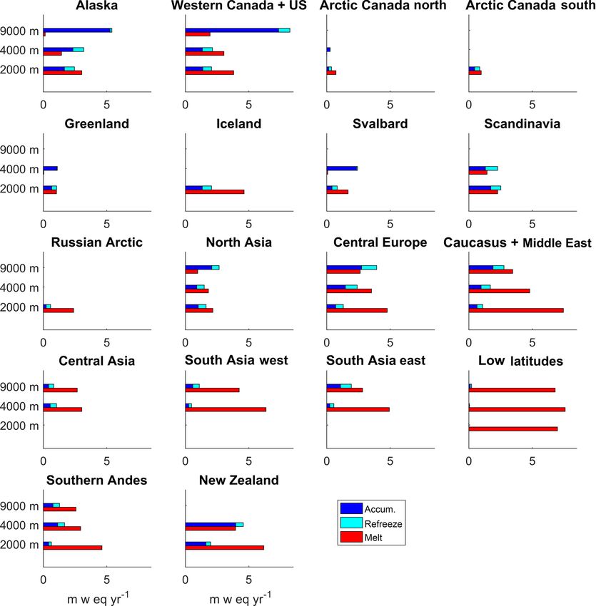
332                                                                         S. Shannon et al.: Global glacier volume projections

Figure 2. The location of mass balance profile observation glaciers from the World Glacier Monitoring Service and the Randolph Glacier
Inventory regions (version 6.0).

Table 2. Best parameter sets for each RGI6 region. The regions are ranked from the lowest to the highest RMSE. There are no observed
profiles for Iceland and the Russian Arctic, so the global mean parameter values are used (bold) for the future simulations.

             Region                          αvis,snow   αnir,snow   αvis,ice   αnir,ice     γtemp        γprecip   γwind
                                                                                           K km−1    % per 100 m
             Arctic Canada south                  0.94        0.77      0.68       0.53        8.3            16     2.15
             Arctic Canada north                  0.96        0.70      0.49       0.12        4.2             7     1.10
             Greenland                            0.95        0.72      0.41       0.19        8.0            15     1.07
             Alaska                               0.88        0.65      0.56       0.27        8.2            16     1.32
             South Asia east                      0.91        0.73      0.67       0.56        5.3             9     1.55
             South Asia west                      0.99        0.73      0.60       0.30        4.0            24     1.69
             Western Canada and the US            0.97        0.64      0.45       0.26        9.3             8     2.29
             Central Asia                         0.94        0.74      0.69       0.50        8.1            19     1.40
             North Asia                           0.94        0.74      0.69       0.50        8.1            19     1.40
             Central Europe                       0.83        0.63      0.59       0.35        5.8             7     1.83
             Svalbard                             0.95        0.76      0.54       0.35        9.0            14     1.02
             Caucasus and the Middle East         0.90        0.71      0.53       0.28        8.3             5     3.32
             Scandinavia                          0.95        0.76      0.54       0.35        9.0            14     1.02
             New Zealand                          0.94        0.74      0.69       0.50        8.1            19     1.40
             Low latitudes                        0.94        0.74      0.69       0.50        8.1            19     1.40
             Southern Andes                       0.95        0.76      0.54       0.35        9.0            14     1.02
             Mean                                 0.93        0.72      0.58       0.37       7.55            14     1.56

itation gradient for each RGI6 region and do not apply a bias        In those studies, the precipitation at the top of the glacier was
correction. A bias correction is often recommended because           estimated using a bias correction factor kp . The decrease in
precipitation is underestimated in coarse-resolution datasets.       precipitation from the top of the glacier to the snout was cal-
Gauging observations are sparse in high-mountain regions             culated using a precipitation gradient. To account for the fact
and snowfall observations can be susceptible to undercatch           that the mass balance of maritime and continental glaciers
by 20 %–50 % (Rasmussen et al., 2012). Our precipitation             responds differently to precipitation changes, kp was related
rates are generally too low because we do not bias-correct           to a continentality index. Our motivation for using a single
the precipitation.                                                   precipitation gradient for each RGI6 region and no bias cor-
   Other studies use a bias correction that varies regionally        rection was to test the simplest approach first; however the re-
(Radić and Hock, 2011; Radić et al., 2014; Bliss et al., 2014).    sulting biases suggest that this approach could be improved.

The Cryosphere, 13, 325–350, 2019                                                            www.the-cryosphere.net/13/325/2019/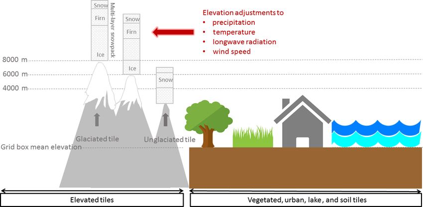
S. Shannon et al.: Global glacier volume projections                                                                                         333

Figure 3. Modelled annual elevation-dependent specific mass balance against observations from the WGMS. The modelled mass balance is
simulated on a 0.5◦ grid resolution at 250 m elevation bands and the observations are for individual glaciers at elevation levels specific to each
glacier. The observed mass balance is interpolated onto the JULES elevation bands. If only a single observation exists, then mass balance for
the nearest JULES elevation band is used. The number of glaciers is shown in the top left-hand corner and the number of observation points
in brackets. In central Europe mass balance for the Maladeta glacier in the Pyrenees is shown in black circles.

   The impact of underestimating the precipitation is that we              show the summer mass balance components for the same two
simulate negative mass balance in winter at some observa-                  glaciers in Fig. S10. Positive mass balance is simulated at
tional sites (Figs. 5a and 4). To demonstrate this, we com-                Kozelsky glacier because accumulation exceeds the melting.
pare the mass balance components for two glaciers: the Leviy               This suggests that the precipitation gradient (19 % per 100 m
Aktru in the Russian Altai Mountains, which has negative                   for north Asia) is overly steep in the summer at this location.
mass balance in the winter, and Kozelsky glacier in north-                    Another reason we underestimate the accumulation is due
eastern Russia, which has no negative mass balance in the                  to the partitioning of rain and snow based on an air temper-
winter (See Fig. S9). Both glaciers are in the north Asia RGI6             ature threshold of 0 ◦ C. The 0 ◦ C threshold is likely too low,
region, so they have the same tuned parameters for mass                    resulting in an underestimate of snowfall. When precipita-
balance. The simulated winter accumulation rates are much                  tion falls as rain or snow it adds liquid water or ice to the
lower at Leviy Aktru glacier than Kozelsky glacier, leading                snowpack. The specific heat capacity of the snowpack is a
to negative mass balance at the lowest three model levels be-              function of the liquid water (Wk ) and ice content (Ik ) in each
low 2750 m.                                                                layer (k)
   The simplistic treatment of the precipitation lapse rate also
                                                                           Ck = Ik Cice + Wk Cwater ,                                        (17)
leads to instances in which the model simulates positive mass
balance in the summer at some locations (Figs. 6a and 4). We               where Cice   = 2100 JK−1 kg−1and Cwater         = 4100 JK−1 kg−1 .
                                                                           The liquid water content is limited by the available pore

www.the-cryosphere.net/13/325/2019/                                                                   The Cryosphere, 13, 325–350, 2019
334 S. Shannon et al.: Global glacier volume projections
Table 3. Root-mean-square error (RMSE), correlation coefficient (r), Nash–Sutcliffe efficiency coefficient (NS), mean bias (Bias), and the
number of elevation-band mass balance observations (No. of obs) for RGI6 regions. The regions are ranked from the lowest to the highest
RMSE.
Region RMSE r NS Bias No. of obs
m w.e. yr−1 m w.e. yr−1
Arctic Canada south 0.96 0.61 0.11 0.10 72
Arctic Canada north 1.06 0.19 −0.44 0.52 1332
Greenland 1.09 0.66 0.14 0.14 90
Alaska 1.36 0.65 0.38 0.06 217
South Asia east 1.41 0.15 −0.34 −0.19 81
South Asia west 1.53 0.62 0.38 −0.09 168
Western Canada and the US 1.73 0.69 0.41 −0.40 916
Central Asia 1.81 0.22 −1.15 −0.51 2519
North Asia 1.95 0.45 −0.04 −0.21 1335
Central Europe 2.03 0.26 −0.65 0.30 9561
Svalbard 2.16 0.36 −6.86 −1.21 1647
Caucasus and the Middle East 2.23 0.30 −0.89 0.33 687
Scandinavia 2.40 0.53 0.20 0.67 10 617
New Zealand 2.57 0.58 −0.30 −1.09 45
Low latitudes 3.06 0.36 −0.71 −0.88 1016
Southern Andes 3.33 0.26 −12.33 −2.87 118
Global 2.16 0.40 −0.11 0.19 30 421
Figure 4. Comparison between modelled and observed elevation-band specific mass balance for winter (grey triangles) and summer (black
dots). The modelled mass balance is calculated using the tuned regional parameters from the calibration procedure.
The Cryosphere, 13, 325–350, 2019 www.the-cryosphere.net/13/325/2019/S. Shannon et al.: Global glacier volume projections 335
Table 4. Winter (bold) and summer number of elevation-band mass balance observations (No. of obs), root-mean-square error (RMSE),
correlation coefficient (r), Nash–Sutcliffe efficiency coefficient (NS), and mean bias (Bias).
Region No. of obs RMSE m w.e. yr−1 r NS Bias m w.e. yr−1
Alaska 127 127 1.82 2.43 0.38 0.76 –7.54 −2.88 –0.29 −2.09
Western Canada and the US 767 729 1.76 2.96 0.53 0.72 –2.68 −2.25 –0.34 −2.28
Arctic Canada north 49 50 0.08 1.09 0.09 0.86 –0.94 −5.01 0.04 −0.79
Greenland 28 36 0.78 3.45 0.33 0.81 –11.31 −11.13 –0.11 −2.40
Svalbard 1122 1126 0.61 2.25 0.18 0.66 –3.90 −12.59 –0.38 −1.84
Scandinavia 5347 10 679 1.52 1.69 0.61 0.78 –0.78 0.32 –0.68 −0.77
North Asia 854 828 1.54 4.15 0.71 0.20 –0.40 −3.81 –1.08 −2.63
Central Europe 5496 4804 1.21 2.77 0.12 0.33 –5.83 −4.63 –0.02 −1.11
Caucasus & the Middle East 602 677 1.39 2.30 –0.12 0.55 –1.15 −0.94 –0.23 −1.18
Central Asia 1778 1751 1.34 4.87 0.21 0.31 –10.57 −16.92 –0.19 −4.23
Southern Andes 34 22 4.19 4.11 –0.81 −0.08 –36.73 −55.59 –3.81 −2.36
New Zealand 45 45 3.37 6.17 0.42 0.32 –10.63 −17.82 –0.01 −5.87
Global 16 249 20 874 1.38 2.16 0.49 0.78 –1.16 0.11 –0.37 −0.92
Figure 5. Simulated and observed elevation-dependent winter mass Figure 6. Simulated and observed elevation-dependent summer
balance when grid boxes with a glacier area of less than 100, 300, mass balance when grid boxes with a glacier area of less than 100,
and 500 km2 are excluded. The colour identifies the RGI6 regions 300, and 500 km2 are excluded. The colour identifies the RGI6 re-
shown in Fig. 2. The RMSE, correlation coefficient, and number of gions shown in Fig. 2. The RMSE, correlation coefficient, and num-
glaciers are listed. ber of glaciers are listed.
space in the snowpack; therefore changes in the snowfall (ice
content) control the overall heat capacity. The underestimate (Marzeion et al., 2012). An improved approach would use
in the ice content reduces the heat capacity, which causes the wet-bulb temperature to partition rain and snow, which
more melting than observed. would include the effects of humidity on temperature. Alter-
Other modelling studies have used higher air tempera- natively, a spatially varying threshold based on precipitation
ture thresholds: 1.5 ◦ C (Huss and Hock, 2015; Giesen and observations could be used. Jennings et al. (2018) showed,
Oerlemans, 2012), 2 ◦ C (Hirabayashi et al., 2010), and 3 ◦ C by analysing precipitation observations, that the temperature
www.the-cryosphere.net/13/325/2019/ The Cryosphere, 13, 325–350, 2019336 S. Shannon et al.: Global glacier volume projections
Table 5. List of high-end climate change CMIP5 models that are (GFDL-ESM2M) (Table 5). The models also cover a range
downscaled using HadGEM3-A. The years when the CMIP5 mod- of extreme wet or dry climate conditions. This is important
els pass +1.5, +2, and +4 ◦ C global average warming relative to to consider for glaciers in the central and eastern Himalayas,
the pre-industrial period are shown. which accumulate mass during the summer months due to
monsoon precipitation (Ageta and Higuchi, 1984) and be-
CMIP5 Ensemble +1.5 ◦ C +2 ◦ C +4 ◦ C
cause future monsoon precipitation is highly uncertain in the
model member
CMIP5 models (Chen and Zhou, 2015).
IPSL-CM5A-LR r1i1p1 2015 2030 2068 The HadGEM3-A data are bias-corrected using a trend-
GFDL-ESM2M r1i1p1 2040 2055 2113*
HadGEM2-ES r1i1p1 2027 2039 2074
preserving statistical bias method that was developed for
IPSL-CM5A-MR r1i1p1 2020 2034 2069 the first Inter-Sectoral Impact Model Intercomparison Project
MIROC-ESM-CHEM r1i1p1 2023 2035 2071 (ISIMIP) (Hempel et al., 2013). This technique uses WATCH
HELIX ACCESS1-0 r1i1p1 2034 2046 2085 forcing data (Weedon et al., 2011) to correct offsets in air
pressure, temperature, longwave and shortwave downward
* No data are available for 2113 because the bias-corrected data end at 2097.
surface radiation, rainfall, snowfall, and wind speed but not
specific humidity. The method adjusts the monthly mean and
threshold varies spatially and is generally higher for conti- daily variability in the GCM variables but still preserves the
nental climates than maritime climates. long-term climate signal. The HadGEM3-A was bilinearly
Winter mass balance is simulated better than summer mass interpolated from its native resolution of N216 (∼ 60 km),
balance, which is seen by the lower root-mean-square errors onto a 0.5◦ grid, to match the resolution of the WATCH
for winter in Table 4. Furthermore, the biases are larger in the forcing data, which were used for the bias correction. The
summer than in the winter (Table 4). It is likely that the sim- daily bias-corrected surface fields from the HadGEM3-A are
ple albedo scheme, which relates albedo to the density of the used to run JULES offline to calculate future glacier volume
snowpack surface, performs better in the winter when snow changes. The bias correction was only applied to data up un-
is accumulating than in summer when there is melting. Fig- til the year 2097, which means the glacier projections termi-
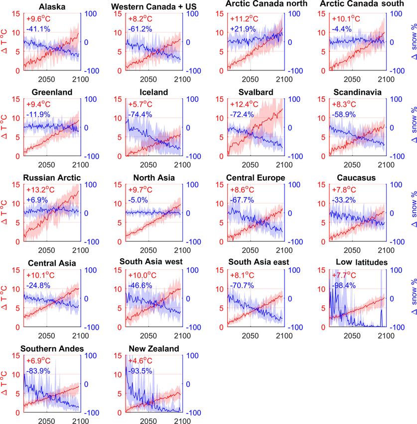
ures 5b–d and 6b–d show the winter and summer mass bal- nate at this year. A flow chart of the experimental setup is
ances for all observation sites when area thresholds of 100, shown in Fig. 7. The HadGEM3-A climate data were gen-
300, and 500 km2 are applied to the validation. There is an erated and bias-corrected for the High-End cLimate Impact
improvement in the simulated summer mass balance when and eXtremes (HELIX) project.
the glaciated area increases. This is seen by the improved
correlation in Fig. 6d in which the validation is repeated but 4.2 Regional glacier volume projections 2011–2097
only grid boxes with a glaciated area greater than 500 km2
are considered. This indicates the model is better at simulat- Glaciated areas are divided into 18 regions defined by the
ing summer melting over regions with a large ice extent than RGI6 with no projections made for Antarctic glaciers be-
over regions with a small glaciated area. cause the bias correction technique removes the HadGEM3-
A data from this region. JULES is run for this century (2011
to 2097) using the best regional parameter sets for mass bal-
4 Glacier volume projections ance found by the calibration procedure (Table 2). No ob-
servations were available to determine the best parameters
4.1 Downscaled climate change projections for Iceland and the Russian Arctic; therefore global mean
parameter values are used for these regions. End of the cen-
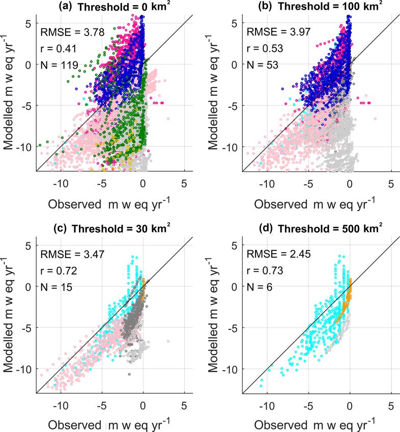
Glacier volume projections are made for all regions, exclud- tury volume changes (in percent) are found by comparing
ing Antarctica, for a range of high-end climate change sce- the volume at the end of the run (2097) to the initial vol-
narios. This is defined as climate change that exceeds 2 and ume calculated from the RGI6. Regional volume changes
4 ◦ C global average warming, relative to the pre-industrial expressed in percent for low (0–2000 m), medium (2250–
period (Gohar et al., 2017). Six models fitting this crite- 4000 m), high (4250–9000 m), and all elevation ranges (0–
rion were selected from the Coupled Model Intercompari- 9000 m) are listed in Table 6. The total volume loss over
son Project Phase 5 (CMIP5). A new set of high-resolution all elevation ranges is also listed in millimetres of sea level
projections were generated using the HadGEM3-A Global equivalent in Table 6 and plotted in Fig. 10. Maps of the
Atmosphere (GA) 6.0 model (Walters et al., 2017). The sea percentage volume change at the end of the century, rela-
surface temperature and sea ice concentration boundary con- tive to the initial volume, are contained in the Supplement in
ditions for HadGEM3-A are supplied by the CMIP5 mod- Figs. S1–S7.
els. All models use the RCP8.5 “business as usual” scenario A substantial reduction in glacier volume is projected for
and cover a wide range of climate sensitivities, with some all regions (Fig. 8). Global glacier volume is projected to de-
models reaching 2 ◦ C global average warming relative to the crease by 64 ± 5 % by end of the century, for which the value
pre-industrial period, quickly (IPSL-CM5A-LR) or slowly corresponds to the multi-model mean ± 1 standard devia-
The Cryosphere, 13, 325–350, 2019 www.the-cryosphere.net/13/325/2019/S. Shannon et al.: Global glacier volume projections 337
Table 6. Percentage ice volume loss, relative to the initial volume (1V ), and ice loss in millimetres of sea level equivalent (SLE) for the end
of the century (2097). Percentage volume losses are shown for low, medium, and high elevation ranges as well as for all elevations. The data
show the multi-model mean ± 1 standard deviation. The conversion of volume to SLE assumes an ocean area of 3.618 × 10⁸ km2 . The initial
area and volume from the Randolph Glacier Inventory version 6 are listed in columns 1 and 2.
Area Volume 1V 0–9000 m 1V 0–2000 m 1V 2250–4000 m 1V 4250–8000 m SLE
km2 km3 % % % % mm SLE
Alaska 86 616 19 743 −89 ± 2 −93 ± 1 −55 ± 9 408 ± 18 44.6 ± 1.1
Western Canada and the US 14 357 1070 −100 ± 0 −100 ± 0 −99 ± 0 684 ± 136 2.8 ± 0.0
Arctic Canada north 104 920 32 376 −47 ± 3 −43 ± 4 40 ± 1 – 35.8 ± 3.0
Arctic Canada south 40 861 9780 −74 ± 8 −72 ± 9 – – 18.1 ± 2.1
Greenland 126 143 29 856 −31 ± 5 −31 ± 6 37 ± 3 – 20.1 ± 4.4
Iceland 11 052 3722 −98 ± 3 −98 ± 3 – – 9.3 ± 0.3
Svalbard 33 932 10 112 −68 ± 16 −65 ± 18 608 ± 158 – 17.0 ± 4.6
Scandinavia 2948 244 −98 ± 3 −97 ± 3 −92 ± 17 – 0.6 ± 0.0
Russian Arctic 51 552 16 908 −79 ± 10 −77 ± 11 – – 33.3 ± 4.8
North Asia 2400 156 −71 ± 5 −97 ± 2 −52 ± 8 220 ± 41 0.3 ± 0.0
Central Europe 2091 127 −99 ± 0 −100 ± 0 −99 ± 0 −77 ± 24 0.3 ± 0.0
Caucasus & the Middle East 1305 71 −100 ± 0 −100 ± 0 −100 ± 0 −99 ± 0 0.2 ± 0.0
Central Asia 48 415 3849 −80 ± 7 – −100 ± 0 −74 ± 9 8.0 ± 0.7
South Asia west 29 561 3180 −98 ± 1 – −100 ± 0 −98 ± 1 8.1 ± 0.1
South Asia east 11 148 773 −95 ± 2 – −100 ± 0 −95 ± 2 1.9 ± 0.0
Low latitudes 2341 88 −100 ± 0 −100 ± 0 −100 ± 0 −100 ± 0 0.2 ± 0.0
Southern Andes 29 369 5701 −98 ± 1 −99 ± 1 −74 ± 14 −57 ± 12 14.4 ± 0.1
New Zealand 1161 65 −88 ± 5 −100 ± 0 71 ± 62 – 0.1 ± 0.0
Global 600 172 137 821 −64 ± 5 −61 ± 6 −36 ± 3 −84 ± 5 215.2 ± 21.3
tion. The regions which lose more than 75 % of their vol-
ume by the end of the century are Alaska (−89 ± 2 %), west-
ern Canada and the US (−100 ± 0 %), Iceland (−98 ± 3 %),
Scandinavia (−98 ± 3 %), the Russian Arctic (−79 ± 10 %),
central Europe (−99 ± 0 %), Caucasus (−100 ± 0 %), central
Asia (−80 ± 7 %), South Asia west (−98 ± 1 %), South Asia
east (−95 ± 2 %), low latitudes (100 ± 0 %), southern Andes
(−98±1 %), and New Zealand (−88±5 %). The HadGEM3-
A forcing data show these regions experience a strong warm-
ing. In most regions this is combined with a reduction in
snowfall relative to the present day, which drives the mass
loss (Fig. 9). Regions most resilient to volume losses are
Greenland (−31±5 %) and Arctic Canada north (−47±3 %).
In the case of Arctic Canada north, snowfall increases rel-
ative to the present day, which helps glaciers to retain their
mass. There is a rapid loss of low-latitude glaciers, which has
also been found by other global glacier models (Marzeion
et al., 2012; Huss and Hock, 2015). Our model overesti-
mates the melting of these glaciers for the calibration period
(Fig. 3), so this result should be treated with a degree of cau-
tion. Some of the high-latitude regions, particularly Alaska,
western Canada and the US, Svalbard, and north Asia, ex-
perience very large volume increases at their upper elevation
ranges. This would be reduced if the model included glacier
dynamics, because ice would be transported from higher el-
Figure 7. Flow chart showing the experimental setup to calculate
future glacier volume. * The bias correction method is described by evations to lower elevations. The ensemble mean global sea
Hempel et al. (2013). level equivalent contribution is 215.2 ± 21.3 mm. The largest
contributors to sea level rise are Alaska (44.6±1.1 mm), Arc-
tic Canada north and south (34.9±3.0 mm), the Russian Arc-
www.the-cryosphere.net/13/325/2019/ The Cryosphere, 13, 325–350, 2019338 S. Shannon et al.: Global glacier volume projections Figure 8. Regional glacier volume projections using the HadGEM3-A ensemble of high-end climate change scenarios. tic (33.3 ± 4.8 mm), Greenland (20.1 ± 4.4), high-mountain the ice is heating up, emitting radiation in the infrared part of Asia (combined central Asia and South Asia east and west), the spectrum. (18.0 ± 0.8 mm), southern Andes (14.4 ± 0.1 mm), and Sval- The downward and upward longwave radiation are in- bard (17.0±4.6 mm). These are the regions which have been creasing in the future; however, the net longwave radiation observed by the Gravity Recovery and Climate Experiment contribution to the melting is small. The downward long- (GRACE) satellite to have lost the most mass in the recent wave radiation increases because of the T 4 relationship with years (Gardner et al., 2013). air temperature, whereas the upward longwave radiation in- To investigate which parts of the energy balance are driv- creases because the glacier surface is warming. The latent ing the future melt rates, we show the energy balance com- heat flux from refreezing of meltwater and the sensible heat ponents averaged over all regions and all elevation levels in from surface warming are also small components of the net Fig. 11. Future melting is caused by a positive net radiation radiation balance. of approximately 30 W m−2 that is sustained throughout the century. This is comprised of 18 W m−2 net shortwave radi- 4.3 Mass balance components ation, 3 W m−2 net longwave radiation, 5 W m−2 latent heat flux, and 4 W m−2 sensible heat flux. The largest component In this section we examine how the surface mass balance of the radiation for melting comes from the net shortwave components vary with height and how this will change in radiation. The upward shortwave radiation comprises direct the future. Figure 12 shows the accumulation, refreezing, and diffuse components in the VIS and NIR wavelengths. and melting contributions to mass balance averaged over The VIS albedo decreases because melting causes the ice sur- low, medium, and high elevation ranges for the period 1980– face to darken. In contrast, the NIR albedo increases because 2000. Sublimation is excluded because its contribution to The Cryosphere, 13, 325–350, 2019 www.the-cryosphere.net/13/325/2019/
You can also read