Measurement characteristics of an airborne microwave temperature profiler (MTP) - Recent
←
→
Page content transcription
If your browser does not render page correctly, please read the page content below
Atmos. Meas. Tech., 14, 1689–1713, 2021
https://doi.org/10.5194/amt-14-1689-2021
© Author(s) 2021. This work is distributed under
the Creative Commons Attribution 4.0 License.

Measurement characteristics of an airborne microwave
temperature profiler (MTP)
Mareike Heckl1, , Andreas Fix1 , Matthias Jirousek2 , Franz Schreier3 , Jian Xu3 , and Markus Rapp1
1 Institut für Physik der Atmosphäre, Deutsches Zentrum für Luft- und Raumfahrt, Oberpfaffenhofen, Germany
2 Institut für Hochfrequenztechnik, Deutsches Zentrum für Luft- und Raumfahrt, Oberpfaffenhofen, Germany
3 Institut für Methodik der Fernerkundung, Deutsches Zentrum für Luft- und Raumfahrt, Oberpfaffenhofen, Germany

 previously published under the name Mareike Kenntner

Correspondence: Mareike Heckl (mareike.heckl@dlr.de)

Received: 27 November 2019 – Discussion started: 8 January 2020
Revised: 3 November 2020 – Accepted: 13 December 2020 – Published: 1 March 2021

Abstract. The microwave temperature profiler (MTP), an             temperatures around flight level (closely related to the ab-
airborne passive microwave radiometer, measures radiances,         solute temperature close to the instrument) with a precision
recorded as counts and calibrated to brightness temperatures,      of 0.38 K. Furthermore, radiative transfer simulations, using
in order to estimate temperature profiles around flight alti-      the Py4CAtS package in a pencil-beam approach, indicate
tude. From these data, quantities such as potential tempera-       that the altitude range of the sensitivity of the MTP instru-
ture gradients and static stability, indicating the state of the   ment can be increased by applying a modified measurement
atmosphere, can be derived and used to assess important dy-        strategy.
namical processes (e.g., gravity waves or stability assess-           This is the first time such an extensive characterization of
ments). DLR has acquired a copy of the MTP from NASA–              an MTP instrument, including a thorough calibration strategy
JPL, which was designed as a wing-canister instrument and is       assessment, has been published. The presented results, rele-
deployed on the German High Altitude LOng range research           vant for the wing-canister design of the MTP instrument, are
aircraft (HALO). For this instrument a thorough analysis of        important when processing MTP data: knowledge of the rel-
instrument characteristics has been made in order to correctly     evant uncertainties and instrument characteristics is essential
determine the accuracy and precision of MTP measurements.          for retrieval setup and is mandatory to correctly identify and
   Using a laboratory setup, the frequency response function       interpret significant atmospheric temperature fluctuations.
and antenna diagram of the instrument were carefully char-
acterized. A cold chamber was used to simulate the changing
in-flight conditions and to derive noise characteristics as well
as reliable calibration parameters for brightness temperature      1   Introduction
calculations, which are compared to those calculated from
campaign data.                                                     Aircraft campaigns have long been used to study atmospheric
   The MTP shows quite large changes in the instrument             composition and dynamics. Here, one important variable to
state, imposing considerable changes in calibration param-         be determined is the atmospheric temperature, ideally not
eters over the course of a single measurement flight; using        only at flight level, as provided in high resolution by the stan-
a built-in heated target for calibration may yield large er-       dard aircraft instrumentation. For this measurement it is de-
rors in brightness temperatures due to a misinterpretation         sirable to use a remote sensing technique that provides good
of the measured absolute temperature. Applying the correc-         horizontal and vertical resolution. A variety of instruments
tions presented herein to the calibration parameter calcula-       and techniques exists; many of them are used in ground-
tions, the measurement noise becomes the dominant source           based setups or installed on satellites. For aircraft instru-
of uncertainty and it is possible to measure the brightness        ments, the line of sight is always an important factor, as
                                                                   is the ability to record data fast (providing high horizontal

Published by Copernicus Publications on behalf of the European Geosciences Union.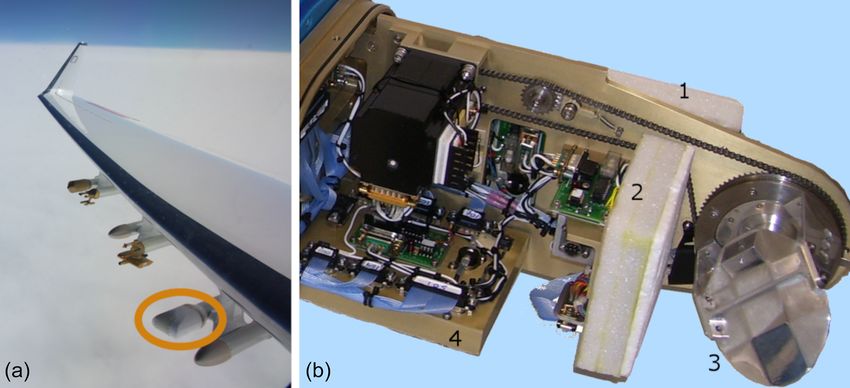
1690                        M. Heckl et al.: Measurement characteristics of an airborne microwave temperature profiler

resolution). It is desirable to use a robust instrument design    tion to tropical weather disturbances (Davis et al., 2014).
able to perform despite frequent changes in conditions due        Furthermore, MTP measurements have been utilized to in-
to flight patterns and geographical regions of deployment.        vestigate gravity waves in the atmosphere. Studies have fo-
On the German High Altitude LOng range research aircraft          cused on general overviews (Gary, 2006, 2008), the forma-
(HALO; Krautstrunk and Giez, 2012), the microwave tem-            tion of polar stratospheric clouds (PSCs; Murphy and Gary,
perature profiler (MTP; Denning et al., 1989) complements         1995; Tabazadeh et al., 1996), and the characterization of
other instruments such as the Basic HALO Measurement and          gravity waves encountered during flight (Gary, 1989; Chan et
Sensor System (BAHAMAS), which measures the tempera-              al., 1993; Dean-Day et al., 1998; Wang et al., 2006). Based
ture amongst other parameters at flight level, and dropson-       on these mesoscale temperature fluctuation analyses, a num-
des. In contrast to such in situ instruments, the MTP scans       ber of modeling studies aimed at improving the understand-
through the atmosphere at different viewing directions, pro-      ing and numerical description of atmospheric gravity waves
viding temperature profile information at, above, and be-         were published, including studies by Bacmeister et al. (1990,
low flight level. A copy of this compact wing-canister in-        1996, 1999), Pfister et al. (1993), Cho et al. (1999), Leut-
strument, which was originally designed by NASA–JPL, has          becher and Volkert (2000), Dörnbrack et al. (2002), and
been transferred to DLR and was modified and certified for        Eckermann et al. (2006). Especially for studies focusing on
operation on HALO. On that aircraft it constitutes a valuable     mesoscale temperature fluctuations or vertical temperature
addition to the scientific payload as the data recorded by the    gradients, precise knowledge of the instrument characteris-
MTP facilitate the interpretation of trace gas measurements       tics, such as intrinsic noise and the precision of the measure-
taken during flight (e.g., by indicating tropopause height and    ments, is necessary, e.g., when identifying potential gravity
static stability) and increase the atmospheric region over        wave signals within the time series of MTP data. Knowing
which information can be gathered. Combining MTP and              the true range of sensitivity is also necessary to understand
dropsonde data (e.g., for cross-validation) or exploiting the     the shape and characteristic structures within the retrieved
synergy with the airborne multi-wavelength water vapor dif-       temperature profiles.
ferential absorption lidar (WALES; Wirth et al., 2009) offers        Despite the continuous use of data from various MTP in-
the opportunity to increase the insight into atmospheric pro-     struments in many studies over the past decades, a thorough
cesses targeted during measurement flights. Its observation       instrument characterization and estimation of measurement
range at, above, and below flight level plus its small size and   accuracy (i.e., the deviation from the true value; mostly influ-
weight clearly set the MTP apart from the HALO Microwave          enced by systematic errors) and precision (i.e., the spread of
Package (HAMP; Mech et al., 2014), which is another op-           the individual measurements; mostly influenced by random
tional instrument package deployable in HALO’s belly pod          errors, such as measurement noise) have not yet been pub-
capable of retrieving both humidity and temperature profiles,     lished. For the first time, this study presents a thorough inves-
as well as the liquid water path (Jacob et al., 2019), below      tigation of relevant instrument characteristics of the HALO
flight level by means of passive microwave radiometry.            MTP instrument. All measurements shown in the following
   The value of MTP data is also demonstrated by its con-         sections are important to correctly choose retrieval settings
tinued use in many aircraft campaigns. Since its invention in     and interpret time series of MTP data. They were conducted
the late 1970s, the MTP has been deployed in a number of          without disassembling the instrument, provided that the hard-
aircraft campaigns (Mahoney and Denning, 2009) and con-           ware characteristics are comparable to previous mission de-
tinues to be developed to meet today’s standards of techni-       ployments, thereby guaranteeing the continued airworthiness
cal requirements and data recording. In the past, MTP data        of the instrument on the HALO aircraft. Knowing the instru-
have been used to interpret in situ measurements of trace         ment characteristics is the foundation for correct analysis and
gases (e.g., Marcy et al., 2007; Thornton et al., 2007; Spinei    interpretation of data recorded by the HALO MTP. The fol-
et al., 2015) and aerosols, (e.g., Gamblin et al., 2006; Popp     lowing sections present a brief description of the instrument
et al., 2006; Schwarz et al., 2008), as well as to assist the     and its measuring principle (Sect. 2), measurements of the in-
study of cloud physics (e.g., Corti et al., 2008; Jensen et       strument response function, the antenna diagram, and other
al., 2010; Schumann et al., 2017; Urbanek et al., 2017) and       inherent characteristics, such as measurement noise (Sect. 3),
dynamics in the atmosphere (e.g., Tuck et al., 1997, 2003;        and a discussion of calibration strategies to determine the
Dörnbrack et al., 2002; Sitnikova et al., 2009). Other stud-      best practice (Sect. 4), including a discussion of the influ-
ies, focusing exclusively on MTP data, include the deriva-        ence of flight-level changes on the instrument state and mea-
tion of the boundary layer height from MTP potential tem-         surement performance. Further error sources and some dis-
perature isentropes (Nielsen-Gammon et al., 2008), inves-         cussion of possible improvements to the measurement strat-
tigation of mixing processes within the polar vortex (Hart-       egy are presented in Sect. 5. The findings are summarized in
mann et al., 1989), and calculation of the cold point tem-        Sect. 6.
perature and mesoscale temperature fluctuations, derived as
the difference to the mission average temperature, in the up-
per troposphere and lower stratosphere (UTLS) in connec-

Atmos. Meas. Tech., 14, 1689–1713, 2021                                            https://doi.org/10.5194/amt-14-1689-2021
M. Heckl et al.: Measurement characteristics of an airborne microwave temperature profiler                                            1691

                                                                            many radiometers measuring atmospheric temperature, the
                                                                            MTP uses absorption lines of the 60 GHz oxygen complex
                                                                            (“V band”), which are caused by magnetic dipole transitions
                                                                            (Liebe et al., 1992). Passive radiometers pick up the energy
                                                                            transported by the photons emitted in these transitions. In this
                                                                            part of the spectrum, the Rayleigh–Jeans relation (e.g., Ulaby
                                                                            et al., 1981) can be used to describe the source function of the
                                                                            radiance picked up by the MTP:

                                                                                          2hν 3        1       ∼  ν2
                                                                            B (ν, T ) =      2
                                                                                                ·            = 2 2 · kB T ,           (1)
Figure 1. HALO MTP instrument. (a) Position of the MTP under-                              c      exp khν   −1    c
                                                                                                       BT
neath the wing of the HALO aircraft. (b) MTP sensor unit in the
lab. Marked with numbers are the radiometer unit (1), the hot cali-         in which the measured radiance is equal to the brightness
bration target (2), the rotating mirror (3), and the electronic unit (4),   B of a black body described by Planck’s law. This equation
which contains various temperature sensors such as the scanning             implies a linear relationship between the measured radiance
unit temperature and the pod air temperature sensor.                        and the temperature T of the black body source at a certain
                                                                            frequency ν using the Planck constant, h, velocity of light,
                                                                            c, and the Boltzmann constant kB . This temperature, T , is
2     Instrument description                                                referred to as brightness temperature (TB ), which is the tem-
                                                                            perature of on an ideal black body emitting the equivalent
The first MTP instrument was developed in the late 1970s                    radiance. The recorded TB s have to be converted to abso-
by Bruce Gary and Richard Denning at the Jet Propul-                        lute temperature profiles by using a retrieval algorithm that
sion Laboratory (NASA–JPL) for research on clear-air tur-                   utilizes forward radiative transfer calculations, in which, ide-
bulence (CAT; Gary, 1989). Since its first deployment in                    ally, all possible impacts on the measured radiance (e.g., wa-
the Stratospheric–Tropospheric Exchange Project (STEP) in                   ter vapor, nitrous oxide, or hydrometeors) have to be consid-
Australia in 1987, the MTP has been widely regarded as                      ered. For correct interpretation of the fluctuations found in
an instrument providing valuable background information                     the retrieved temperature fields, it is necessary to have pre-
on the state of the atmosphere, and several instrument de-                  cise knowledge of the instrument characteristics, such as the
signs have been realized. The latest development is the MTP                 instrument response function, antenna diagram (see Sect. 3),
as a wing-canister instrument (see Fig. 1a), which can be                   and the precision and accuracy of the brightness temperature
mounted underneath the wing of a research aircraft (e.g.,                   measurements that are input to the retrieval algorithm (see
Haggerty et al., 2014). Two such instruments were built. One                Sect. 4).
has been deployed on the NCAR GV since 2008 (e.g., Lim                         In the MTP instrument, a horn antenna guides the incom-
et al., 2013; Davis et al., 2014; Haggerty et al., 2014), and               ing atmospheric radiation and, together with the hyperbolic
the other (hereafter referred to as the HALO MTP) was ac-                   shape of the rotating mirror, determines the spatial response
quired by DLR and has been flown on the German research                     function. The measurements are based on the heterodyne
aircraft HALO (Krautstrunk and Giez, 2012). This design                     principle, which means that through mixing with a defined
was first introduced in 2008. Details of the instrument de-                 frequency, the local oscillator frequency (LO), the incoming
sign and some discussion on standard measurement settings                   signal is converted to an interim frequency (IF) near base
can be found in Mahoney and Denning (2009) and Lim et                       band. Both difference frequencies below and above the LO
al. (2013).                                                                 frequency are down-converted to the IF in the double-side-
   In the following, an overview of the characteristics of this             band receiver. Low-pass filtering suppresses any incoming
specific version of MTP instruments is given, starting with a               radiation outside the IF bandwidth of 200 MHz such that
brief introduction of the measurement principle followed by                 the symmetric spectrum around the current LO frequency is
a description of specific radiometric hardware (see also Ta-                measured with only a minor gap of approximately 20 MHz
ble 1) built into the HALO MTP. All results in the following                at the LO frequency. The IF signal is converted to a volt-
sections are representative of this specific MTP instrument                 age, which is proportional to the squared input amplitude,
design.                                                                     representing the power. This voltage is finally translated to a
                                                                            digital count number, stored in the MTP data file, and later
2.1    Measurement principle                                                converted into a brightness temperature through calibration
                                                                            (see Sect. 4). The physical temperatures of the important ra-
The concept of measurements by the MTP as a passive                         diometric parts of the radiometer, such as the mixer, synthe-
total-power radiometer (Denning et al., 1989; Ulaby et al.,                 sizer, amplifiers, and the electronics, are stabilized to min-
1981) is straightforward. The MTP records thermal radiation                 imize the influence of the changing conditions during a re-
mainly emitted by oxygen molecules in the atmosphere. Like                  search flight on the instrument state and to protect the elec-

https://doi.org/10.5194/amt-14-1689-2021                                                       Atmos. Meas. Tech., 14, 1689–1713, 2021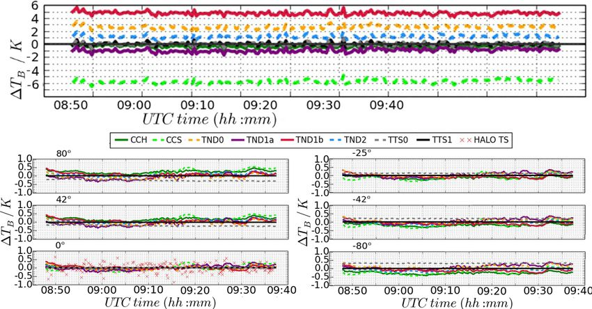
1692                        M. Heckl et al.: Measurement characteristics of an airborne microwave temperature profiler

Table 1. MTP instrument: components and settings.

    Component                Description                                                              Standard settings
    Fairing                  Fiberglass with Al attach fitting to protect the hardware from the en-
                             vironment
    Microwave window         High-density polyethylene, allowing viewing of the atmosphere at
                             ±80◦ range
                             Groves serve as an anti-refraction “coating”
    Rotatable mirror         Aluminum mirror with hyperbolic design to have a beam width of           +80, +55, +42, +25, +12±0,
                             7.5◦ ; 360◦ rotatable                                                    −12, −25, −42, −80◦
                             Stepper motor used: Lin Engineering, CE-5718L, step size: 1.8◦
    Horn antenna             Conical, corrugated feed horn with an orthomode transducer (OMT)
                             attached to the base
    Radiometer parts         Cross-guide coupler for injection of a noise diode calibration signal    Nominal filter bandwidth:
                             Isolator to prevent local oscillator (LO) signal leakage                 ∼ 200 MHz
                             Double-side-band biased mixer
                             Amplification and an interim-frequency (IF) filter to select the pass
                             band
    Frequency synthesizer    Wide band YIG-tuned synthesizer with 1 Hz resolution can be tuned        56.363, 57.612, 58.363 GHz
                             for an output frequency from 12.0 to 16.0 GHz
                             The synthesizer output is doubled twice for a possible LO frequency
                             range of 48–64 GHz
    Reference target         1 in. (∼ 2.54 cm) thick carbon–ferrite mounted on an aluminum plate      Temperature control set to
                             Styrofoam and ROHACELL foam insulation (1/4 in. or ∼ 0.635 cm)           approx. 45 ◦ C at the back of
                             Two conventional power resistors for temperature control; integrated     the target
                             in aluminum plate
    Data                     DC voltage proportional to the brightness temperature in front of the    Recorded using LabView
                             antenna, converted to digital counts                                     software on PC/104
                                                                                                      Integration time (signal record-
                                                                                                      ing): 200 ms
    Housekeeping             Platinum resistance temperature devices (RTDs) at various
                             locations on MTP hardware
    Controller PC            Commercial ultralow-power single-board computer in a PC/104              Connected to HALO network to
                             format with a passive heat sink                                          enable user control if necessary
                             Runs independent from cabin control                                      or wanted

tronic parts from malfunction due to condensation (see Ma-             cycle: five above the horizon, four below, and one pointing
honey and Denning, 2009, for further details).                         exactly towards the horizon. At each angle, measurements
   Using a rotating mirror in front of the instrument’s feed           at three frequency channels, corresponding to the frequen-
antenna (number 3 in Fig. 1b), the direction from which the            cies of three strong oxygen absorption lines, are subsequently
radiation is collected can be changed. Moving through a sin-           performed (see Table 1) before moving to the next elevation.
gle set of elevation angles, as well as the set of frequency              Furthermore, a calibration target is built into the instru-
channels at each of those elevation angles, is referred to in          ment (number 2 in Fig. 1b), to which the mirror points after
the following as a measurement “cycle”. This procedure en-             each cycle of atmospheric measurements. The target itself
hances the vertical resolution of measurements in compar-              consists of carbon–ferrite on an aluminum plate, which is
ison to non-scanning measurements, which derive altitude               heated to a constant temperature (approximately 45 ◦ C) us-
information solely from exploiting frequency-dependent dif-            ing two conventional power resistors. The calibration target
ferences in the optical depth of the atmosphere. The MTP               is surrounded by a 1 in. thick Styrofoam insulation, which
combines both principles. In its standard deployment set-              is transparent for microwave radiation. The signals recorded
tings, as programmed in the original JPL instrument soft-              while pointing towards the heated target are combined with a
ware, 10 viewing angles are used during one measurement                noise diode (ND) signal and used for calibration (see Sect. 4)

Atmos. Meas. Tech., 14, 1689–1713, 2021                                                   https://doi.org/10.5194/amt-14-1689-2021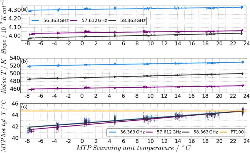
M. Heckl et al.: Measurement characteristics of an airborne microwave temperature profiler                                     1693

to convert the measured signal to a TB , which is usually not       13 mission flights, recording 17 476 individual measurement
equal to the outside air temperature, since the measured sig-       cycles. Data from this campaign will be used to derive the
nal is influenced by multiple layers of the atmosphere. To          HALO MTP noise characteristics and in the investigation of
derive absolute temperature from the radiation measurement,         calibration methods in the following sections.
radiative transfer calculations have to be carried out and com-
pared to the measured radiances by applying a retrieval algo-
rithm in post-processing. The instrument characteristics pre-       3     Characteristics of the wing-canister MTP flown on
sented in the following sections of this work all correspond to           HALO
the raw measurements or the brightness temperatures, which
are input to such a retrieval algorithm. However, a discussion      To retrieve absolute temperature profiles from the MTP mea-
of retrieval algorithms and related uncertainties is beyond the     surements, radiative transfer calculations are carried out to
scope of this paper.                                                model the measured radiance in a defined atmospheric state.
                                                                    To correctly do so, the instrument transmission function (see
2.2   Specific wing-canister instrument hardware                    Fig. 2a) has to be known. This function is defined by the in-
      characteristics                                               strument’s filter function, which determines which part of the
                                                                    recorded spectrum is used in data processing. Moreover, the
Differences to older instrument designs are presented in Lim        antenna diagram (see Fig. 2) shows how sensitive the receiver
et al. (2013) and Haggerty et al. (2014). The most important        is to the different directions it is pointing towards. Both the
upgrade is that the LO is now defined as a frequency near (or       filter functions and the antenna diagram have been measured
ideally at) an oxygen absorption line center so that the two        in a stable laboratory environment (Sect. 3.1).
flanks that are measured belong to the same line, which low-            Since this MTP instrument is mounted to the outside of the
ers the brightness temperature error, as discussed in Mahoney       aircraft (see Fig. 1, left), the instrument experiences changes
and Denning (2009) and Lim et al. (2013). The instrument is         in surrounding pressure and temperature during measure-
pointing forward, measuring the temperatures of air masses          ment flights in which flight-level changes can be quite com-
in front of the aircraft. The filter bandwidth of the HALO          mon. During a single mission flight, the air temperature sur-
MTP is fixed to ±200 MHz around the LO, with a gap of ap-           rounding the aircraft can change from around 300 K on the
proximately 20 MHz at the line center (see Fig. 2a). The syn-       ground to as low as 190 K in the tropopause. These changing
thesizer used to generate the LO for down-conversion of the         ambient temperatures of the MTP can influence the perfor-
signal can be tuned between 12 and 16 GHz. The synthesizer          mance of the instrument: amplifiers might change their char-
output is doubled twice, potentially allowing for a frequency       acteristics, and thus the relation between the recorded signal
range of 48 to 64 GHz for atmospheric measurements. The             and the source temperature, i.e., the calibration parameters,
preset (“standard”) set of LO frequencies used was chosen           change. Moreover, the noise diode used for calibration may
based on the considerations presented in Mahoney and Den-           change its signal strength (see Sect. 4.2), and the overall in-
ning (2009) and Lim et al. (2013). This set of frequencies is       strument noise can be affected. However, the noise character-
used for this study.                                                ization is particularly important when interpreting tempera-
   Two significant modifications to the original instrument         ture fluctuations in a time series of MTP data. Knowing pos-
were made by DLR: an embedded computer and an inertial              sible periodicity in the noise signal is essential to distinguish
measurement system including a Global Positioning System            between real periodic atmospheric temperature fluctuations,
(GPS) antenna. In the original setup a Visual Basic software        e.g., those caused by gravity waves, and instrument noise.
package was provided by NASA–JPL to run the instrument              To test all of these characteristics, the MTP was placed in-
during research flights. With the onboard computer and inte-        side a temperature chamber (Fig. 3) to simulate the chang-
gration of the inertial sensor, this software was translated to a   ing outside air temperature during mission flights. In these
LabView code, which was adjusted to use the additional data         tests, the influence of the changing surrounding temperature
provided by the inertial sensor. With those modifications, the      on the linearity of the sensor is tested (Sect. 3.2), and the
HALO MTP can be operated autonomously, i.e., indepen-               measurements are used to determine the noise characteristics
dent from a connection to a cabin computer, which is still          of the HALO MTP. The laboratory results are also compared
provided and can be used, e.g., to adjust settings during re-       to the noise characteristics derived from airborne ML CIR-
search flights using the HALO LAN network.                          RUS mission data (Sect. 3.3). Possible calibration strategies
   The HALO MTP was first deployed during the Midlati-              and the effect of changing instrument state on the calibration
tude Cirrus Experiment (ML CIRRUS) in 2014 (Voigt et al.,           of data will be discussed in Sect. 4.
2017). The focus of this mission was to probe natural cir-
rus clouds and contrail cirrus throughout various stages of         3.1    Instrument function
their life cycles. The MTP was part of the wing-probe in-
strumentation and recorded data during all mission flights. In      The measurements of the instrument transmission functions,
total, the HALO MTP produced almost 63 h of data during             as well as of the antenna diagram, were made in a cham-

https://doi.org/10.5194/amt-14-1689-2021                                              Atmos. Meas. Tech., 14, 1689–1713, 2021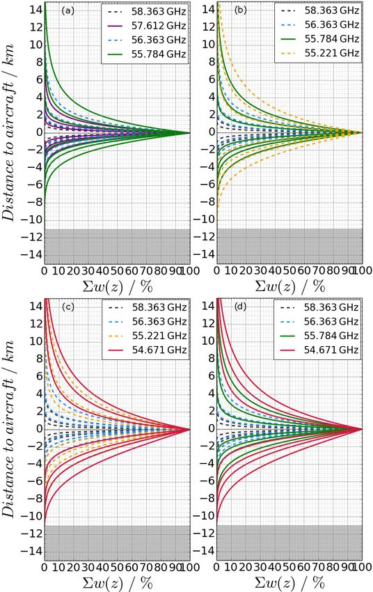
1694 M. Heckl et al.: Measurement characteristics of an airborne microwave temperature profiler
Figure 2. HALO MTP filter functions (a) and antenna diagram of the horizontal (b) and vertical (c) plane recorded at standard measurement
frequencies. Red dashed lines indicate the half-maximum value. All data are normalized so that the maximum value shown is 0.
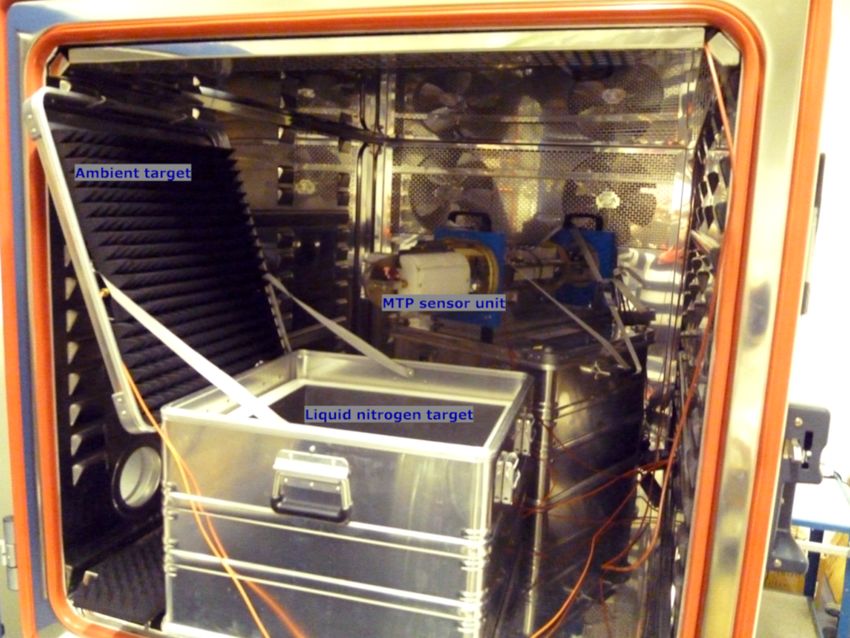
Figure 3. HALO MTP inside the cold chamber. For the measurements, the box containing the liquid nitrogen and the ambient target was
rotated to face towards the MTP sensor unit. A second microwave absorber was placed on the ceiling of the chamber to function as a second
ambient target.
ber completely covered in microwave absorbers. The MTP (e.g., Balanis, 1997):
was installed on a rotatable platform. A tuneable signal countsnorm
source with a horn antenna was placed at 5 m of distance countscorr = . (2)
f 2 /(min (f ))2
to the MTP instrument. The signal was then measured by
the MTP and by a power meter for reference. The power of Finally, the signal power of the source, Pcorr (f ), is taken into
the source signal was chosen such that the MTP signal was account in a final normalized signal representing the relative
well above its inherent noise level. For the measurement of forward transmission, countsfinal :
the filter function, the source frequency was tuned between countscorr
LO − 300 MHz and LO + 300 MHz in steps of 1 MHz. The countsfinal = . (3)
Pcorr (f )
measured signal is normalized and then corrected for fre-
The resulting instrument transmission functions for the three
quency dependency based on the Friis transmission equation
standard frequency channels are shown in Fig. 2a. It shows
Atmos. Meas. Tech., 14, 1689–1713, 2021 https://doi.org/10.5194/amt-14-1689-2021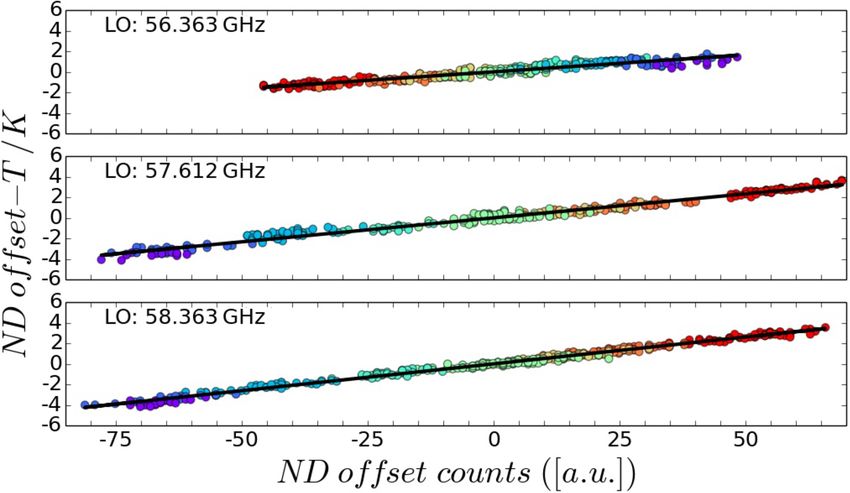
M. Heckl et al.: Measurement characteristics of an airborne microwave temperature profiler                                       1695

symmetrical shapes for all frequency channel functions (i.e.,
radiances are recorded symmetrically from both flanks of the
probed oxygen line), confirming a transmission of the sig-
nal at ±200 MHz around the LO (the width of the plateau).
The gap in the center is created by the receiver architecture
using a double-side-band receiver as explained in Sect. 2. A
certain “waviness” with an amplitude of about 0.5 dB is visi-
ble next to this gap. To exclude reflections from the chamber
as a source, the measurements were repeated multiple times        Figure 4. Temperature sensor measurements during cold-chamber
with slightly different positioning of the source antenna and     measurements (a; black line: scanning unit sensor, blue line: pod
the instrument. Since the results were similar in all measure-    air sensor). At 0 ◦ C (∼ 11:45 UTC) the cold-chamber software had
ments, the source of this waviness is attributed to some inter-   to be restarted, causing a longer stabilization period, and at −5 ◦ C
nal source within the instrument due to electromagnetic wave      (∼ 13:15 UTC) the cold chamber was opened to refill the liquid ni-
propagation through the instrument parts.                         trogen in the cold target, causing spikes in the temperature measure-
   The main result of measuring the antenna diagram is the        ment. (b) Pod air temperature measurements during all ML CIR-
field of view (FOV) of the instrument, defined by the full-       RUS campaign flights.
width half-maximum (FWHM; red dashed lines in Fig. 2b
and c) of the antenna diagrams. It is actually mainly defined
by the hyperbolic shape of the rotating mirror at the front       readings of this sensor give an impression of the state of the
of the instrument. The measurement was made using the             instrument and its thermal stability. It can be seen that the
same laboratory setup as for the measurement of the trans-        response to lowering the cold-chamber temperature is differ-
mission function. Both the horizontal and the vertical plane      ent between the two sensors. This is caused by the placement
were measured in steps of 1◦ rotation. The symmetric shape        of the sensors, with one being closer to some heated parts
of the diagram implies that radiance is picked up equally         of the instrument, indicating that changes in the environment
strong from all directions. Note that the maxima of the side      of the instrument do not equally influence all parts of the in-
lobes in the antenna diagrams have a maximum at −30 dB,           strument. Moreover, from the readings of the scanning unit
meaning the signals from these spatial directions are 1000        temperature sensor (black line in Fig. 4a) it can be seen that
times weaker than the signal picked up from the main view-        the MTP instrument takes some time to stabilize under the
ing direction. The FOV is about 7.0–7.5◦ in the horizontal        new temperature conditions. This time required for stabiliza-
and about 6.5–7.0◦ in the vertical at all frequencies.            tion depends a lot on the operating environment, such as the
   A spillover measurement of the horn antenna (as investi-       size of the laboratory space, ventilation, and ambient tem-
gated, for example, in McGrath and Hewison, 2001) and a           perature. In this setting, it takes up to 15 min after the initial
test of the stability of the LO frequency generator were not      temperature change. Only those parts of the measurement se-
possible, as this would have required disassembling parts of      ries are used in which the scanning unit temperature is stable
the instrument, which was not an option at that time due to       (the difference between two readings being smaller than an
aircraft certification issues.                                    empirical threshold value of 0.04 K) to exclude effects from
                                                                  the instrument adjusting to new environmental conditions.
3.2   Temperature dependence of MTP characteristics                  Along with the MTP instrument two microwave absorbers
                                                                  (Telemeter Electronic GmbH EPP51 broadband pyramidal
To investigate the temperature dependence of instrument per-      absorber) at ambient temperature (hereafter referred to as
formance, a series of measurements inside a cold chamber          “ambient targets”) and a similar microwave absorber sub-
was performed (see Fig. 3). During this measurement series,       merged in liquid nitrogen (hereafter referred to as the “cold
the temperature of the cold chamber was successively low-         target”) were placed in the chamber in order to perform cali-
ered from 21 to −15 ◦ C in steps of 5 ◦ C. This temperature       bration measurements throughout the complete measurement
range resembles the temperatures the MTP experienced dur-         series. The third type of calibration target used in this mea-
ing its deployment in the ML CIRRUS campaign in 2014,             surement series is the built-in calibration target of the MTP
as shown in Fig. 4b. The pod air temperature sensor mon-          instrument (see Sect. 2), hereafter referred to as the “hot tar-
itors the temperature inside the MTP’s housing during the         get”.
flight (see Fig. 1b). In the cold chamber, the housing was not
installed to prevent overheating of the instrument at higher      Linearity of the sensor
temperatures. As a result, the readings of this sensor show
the air temperature inside the cold chamber. The scanning         Using the measurements of the two ambient targets installed
unit temperature sensor keeps track of the temperature of the     within the chamber, it can be shown that for the HALO MTP
MTP instrument within close proximity to the crucial parts        the linear relation between the source temperature and the
of the radiometer, such as the amplifiers and the mixer. The      measurement output is given at all standard frequency chan-

https://doi.org/10.5194/amt-14-1689-2021                                             Atmos. Meas. Tech., 14, 1689–1713, 2021
1696                          M. Heckl et al.: Measurement characteristics of an airborne microwave temperature profiler

                                                                       into account by applying a linear fit to the measured data
                                                                       of one segment (black line in Fig. 6) instead of simply sub-
                                                                       tracting the mean (blue line in Fig. 6). Using all segments of
                                                                       the cold-chamber measurements, the resulting HALO MTP
                                                                       noise characteristics, as shown in Fig. 7 (top), can be de-
                                                                       scribed by a Gaussian distribution with a standard devia-
                                                                       tion of approximately 6 counts (approximately 0.25 K) and
                                                                       a mean of 0 counts.
                                                                           The same method as for the cold-chamber measurements
Figure 5. Ambient target temperature vs. the measured signal           is used for HALO MTP data recorded during the ML CIR-
(counts) of the two ambient targets for all three standard frequency   RUS campaign in 2014. Here, the criterion used to determine
channels of the HALO MTP (different line styles). Different line       flight segments with nearly stable instrument states is a dif-
colors correspond to the measurement of the two individual ambi-       ference in the scanning unit temperature of less than 0.04 K
ent targets.                                                           between two measurement cycles. Additionally, it was en-
                                                                       sured that no altitude changes were made (1z ≤ 25 m) and
                                                                       no curves were flown during these segments. From all ML
nels (see Fig. 5). Fits to the data using higher orders show           CIRRUS mission and test flights, 61 segments could be iden-
that only the linear term significantly contributes to the data        tified that satisfied the criteria and were at least 5 min long
fit. Since the temperature of not only the target, but also the        to ensure significance of statistical results from the length
temperature of the sensor unit itself, changed during this test,       of one segment: with the length of one measurement cycle
which are both monitored (see Fig. 4), it can also be es-              (including a calibration measurement at the end) at 13 s each
tablished that the linear relationship between the measured            segment includes at least 22 recordings of the hot target mea-
signal and the source temperature is maintained through-               surement signal. Figure 7b shows the noise characteristics at
out changing conditions. The measurements corresponding                56.363 GHz. The results from the flight data evaluation are
to the two individual ambient targets (different line colors in        in excellent agreement with the values found in the labora-
Fig. 5) are nearly identical, proving the consistency of mea-          tory environment, showing even smaller standard deviations
surements.                                                             of 5.2–5.7 counts, depending on the frequency channel. This
    The calibration parameters needed to calculate the bright-         is strong evidence that the HALO MTP noise characteristics
ness temperature (TB ) from the measured signal (“counts”; c)          do not change between flights, and laboratory assessment can
are therefore the y intercept (receiver noise temperature; TR )        be used to determine overall instrument health and compara-
and the slope of the line (scal ) drawn through two points de-         bility of measurements between campaigns, also serving as
fined through measurements of calibration targets at known             information for the retrieval development.
temperatures:                                                              For the spectral analysis of the MTP measurement noise
                                                                       the 61 ML CIRRUS mission flight segments are used again.
TB = c · scal − TR .                                            (4)
                                                                       Due to the varying lengths of the individual flight legs, the
In Sect. 4 it will be shown that those parameters depend on            data are concatenated to a single timeline for spectral anal-
the instrument state and can be related to housekeeping data.          ysis. The power spectrum of the noise signal of the HALO
Please note that in the classical microwave notation, the cal-         MTP at 56.363 GHz, as shown in Fig. 7 (bottom), reveals that
ibration is actually defined inversely as TB = c · G + TR , in         the measurement noise can best be described as red noise,
which the gain (G) is equal to the inverse slope as defined in         which is characterized by the autocorrelation α between a
the above equation.                                                    data point of the time series and its precursors. According to
                                                                       Torrence and Compo (1998), the corresponding theoretical
3.3    Noise characterization                                          noise power spectrum for a range of wave numbers k, Pk , is
                                                                       given by
The instrument’s noise was characterized using the signal
                                                                                        1 − α2
measured when pointing towards the hot target. It is as-               Pk =                             .                         (5)
sumed that due to the temperature stabilization of the tar-                   1 + α 2 − 2α cos(2π k/N )
get, the mean measurement signal should not change over                For the three standard frequency channels, the lag-1 auto-
time. Hence, the deviation from the mean represents the noise          correlation of MTP measurements during the ML CIRRUS
added by the instrument. An example of the measured signal             campaign is α ∼ = 0.7. Fit parameters characterizing the noise
while looking at the hot target during one measurement seg-            characteristics at the three standard frequency channels are
ment at constant cold-chamber temperature is shown as the              summarized in Table 2.
grey line in Fig. 6. Obviously, absolute stability can hardly            With the above findings, characterizing the HALO MTP
be reached in a cold environment, while parts of the sen-              measurement noise as Gaussian-shaped, with a mean of
sor unit are heated to approximately 40 ◦ C, which is taken            0 counts and a standard deviation of 6 counts, as well as

Atmos. Meas. Tech., 14, 1689–1713, 2021                                                 https://doi.org/10.5194/amt-14-1689-2021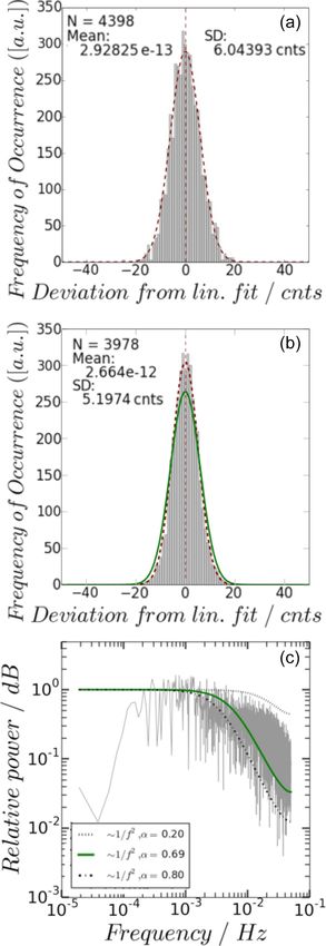
M. Heckl et al.: Measurement characteristics of an airborne microwave temperature profiler                                                 1697

Figure 6. Measured signal (grey line) at 56.363 GHz while looking at the ambient target inside the cold chamber as well as a running average
(light, blue line), mean value (blue line), and linear fit (black line). The corresponding brightness temperature change in the linear fit during
the segment is about 0.8 K.

Table 2. HALO MTP instrument noise characteristics at each of the three standard frequency channels.

                                              56.363 GHz                   57.612 GHz                   58.363 GHz
             Gauss fit: lab measurements      Mean: 2.92825 × 10⁻¹³        Mean: −1.5046 × 10⁻¹²        Mean: −2.64535 × 10⁻¹²
             (N = 4398)                       SD: 6.04393 counts           SD: 6.0963 counts            SD: 6.2264 counts
             Gauss fit: flight data           Mean: 2.664 × 10⁻¹²          Mean: 9.1452 × 10⁻¹⁴         Mean: 3.7587 × 10⁻¹³
             (N = 3978)                       SD: 5.1974 counts            SD: 5.1546 counts            SD: 5.72666 counts
             Autocorrelation (spectral fit)   α = 0.71                     α = 0.70                     α = 0.71

with the knowledge of the inherent periodic structure of the               cies under rapidly changing measurement conditions, which
noise signal, it is now possible to determine whether peri-                could lead to large errors in the calculated TBs. The cold-
odic structures in an MTP temperature measurement time                     chamber measurements described in the previous section are
series are significant (high probability that they result from             used to investigate the influence of the changing instrument
atmospheric temperature fluctuations) or noise-induced. Ad-                state (due to changing surrounding temperature) on the cal-
ditionally, the standard deviation of the Gaussian distribu-               ibration parameters and the ND signal. To determine a best
tion of noise values can be used to determine the variance                 practice for calibration of MTP raw data, various methods
of TBs derived from the raw signals once the calibration pa-               to calibrate HALO MTP data are described in the following,
rameters are known. While it would be interesting to investi-              giving a brief overview of their respective advantages and
gate the integration time needed to significantly reduce the               disadvantages in connection with the HALO MTP.
measurement noise (e.g., by applying the Allen variance),                    1. The first calibration method is hot–cold calibration with
any increase in integration time will decrease the horizon-                     a cold target (microwave absorber submerged in liq-
tal resolution of measurements taken on a jet-engine aircraft.                  uid nitrogen) at temperature Tcold and an ambient tar-
The current settings present a well-chosen compromise be-                       get (microwave absorber at room temperature) at tem-
tween the measurement noise and the horizontal resolution                       perature Tamb to derive the calibration parameters. This
of the MTP data (MJ Mahoney and Richard Denning, pri-                           is the standard calibration method of radiometers in a
vate communication, 2013). As the calibration measurement                       stable environment. Using this method to calibrate the
is already made at the end of each measurement cycle, the in-                   sensor, before or after taking measurements in the at-
strument is calibrated as frequently as possible, and the cal-                  mosphere, provides the calibration parameters based on
ibration performance cannot be further improved by adding                       two temperatures which lie on the upper edge and be-
more calibration measurements during mission flights.                           low the expected measurement range. Thus, the validity
                                                                                of the calibration for the following measurements can
                                                                                be ensured, as long as the sensor itself is in the same
4   Investigation of calibration methods for the HALO                           surrounding conditions during the calibration as dur-
    MTP                                                                         ing the atmospheric measurements and sufficient instru-
                                                                                ment stability is given. Since this stability is not given
In Sect. 3.2 it was shown that there is a linear response in                    for the MTP instrument, the equations applied for this
the measured signal to changes in the source temperature so                     calibration method are the following:
that the measured signal can be related to a brightness tem-
                                                                                 TBCCh (c) = scal
                                                                                              CCh
                                                                                                  (chot ) · c − TRCCh (chot ) ,             (6a)
perature by using the linear relation in Eq. (4). While a line
can be fitted through any two known points, which makes                                 Tamb − Tcold
                                                                                 scal =              ,                                      (6b)
the calibration process very simple, the determination of the                           camb − ccold
calibration parameters also faces the danger of inconsisten-                     TR = Tamb − scal · camb ,                                  (6c)

https://doi.org/10.5194/amt-14-1689-2021                                                       Atmos. Meas. Tech., 14, 1689–1713, 2021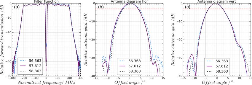
1698                          M. Heckl et al.: Measurement characteristics of an airborne microwave temperature profiler

                                                                           nal used in the second calibration method as described
                                                                           below. However, since it makes use of external cali-
                                                                           bration targets, the calibration measurement can only
                                                                           be performed on the ground, where single calibration
                                                                           measurements at arbitrary room temperatures may not
                                                                           be representative of the instrument state during flight,
                                                                           as shown below. However, this method can be used to
                                                                           check the overall health of the instrument between de-
                                                                           ployments.

                                                                        2. The second calibration method is using the MTP built-
                                                                           in hot target (microwave absorber with a heated metal
                                                                           plate in the back) at temperature Thot combined with a
                                                                           noise diode offset signal cND .

                                                                           TBND (c) = scal · c − (Thot − scal · chot )           (7a)
                                                                                     TND
                                                                           scal =                                                (7b)
                                                                                  cND − chot
                                                                           This is the default way to calibrate MTP measurements.
                                                                           By using calibration measurements taken during flight,
                                                                           the calibration roughly follows the individual state of
                                                                           the instrument, whatever conditions the aircraft meets.
                                                                           The downside of this method is that a faulty noise diode
                                                                           signal can jeopardize reliable calibration. Also, in this
                                                                           method two reference temperatures are used, which are
                                                                           above the expected measurement range: the built-in cal-
                                                                           ibration target is up to 100 K warmer than the outside
                                                                           air temperatures during flight, and TND is added to this
                                                                           temperature. Hence, small uncertainties in the determi-
                                                                           nation of the calibration parameters may lead to large
                                                                           deviations in the calibrated data.

                                                                        3. The third calibration method is using the MTP built-
                                                                           in hot target combined with HALO static temperature
                                                                           (HALO TS) using the equation
Figure 7. HALO MTP noise characteristics at 56.363 GHz. Figures
for the other two standard frequency channels look similar. Fit pa-        TBTS (c) = scal · c − (Thot − scal · chot ) ,         (8a)
rameters for all three frequency channels are summarized in Table 2.              Thot − TS
(a) Laboratory measurements in the cold chamber. Red dashed line:          scal =             .                                  (8b)
Gauss fit to the data. (b) Derived from ML CIRRUS flight data.                    chot − c0◦
Green line: ideal Gauss function with the mean at 0.0 and a standard
                                                                           Here, c0◦ represents the recorded signal at the horizon-
deviation of 6 counts (∼ 0.25 K), as implied by the cold-chamber
                                                                           tal viewing angle, which corresponds to the forward-
noise spectrum. (c) Noise spectrum calculated from ML CIRRUS
flight data. Black dashed lines: theoretical power spectra of 1/f 2        looking measurement, probing the air masses directly in
noise with lag-1 correlations of α = 0.2 and α = 0.8. Green solid          front of the aircraft. This method is an alternative to the
line: theoretical power spectrum of 1/f 2 noise with lag-1 correla-        previous calibration method in the case that the noise
tion of input data.                                                        diode signal cannot be used. It also follows the individ-
                                                                           ual state of the instrument during measurement flights,
                                                                           but since this method uses the HALO static temperature
                                                                           measurement, the MTP data are no longer independent
     in which chot denotes a system parameter that describes               from the aircraft measurements.
     the instrument state (see following section) so that in-
     flight data can be related to the cold-chamber laboratory         Other calibration methods, such as tipping curve calibration
     measurements within a similar instrument state (indi-             (e.g., Küchler et al., 2016; Han and Westwater, 2000), are
     cated by the index CCh). Using the hot–cold calibration           not available for the DLR MTP because of the given instru-
     method is necessary to characterize the noise diode sig-          ment design (mainly antenna beam width) and potentially

Atmos. Meas. Tech., 14, 1689–1713, 2021                                                 https://doi.org/10.5194/amt-14-1689-2021
M. Heckl et al.: Measurement characteristics of an airborne microwave temperature profiler 1699
fast-changing atmospheric conditions due to the moving plat- and the calibration parameters to be used at these tempera-
form, influencing radiative transfer calculations needed in tures. The same is true when using the hot target measure-
this approach and the need for an efficient measurement strat- ment signal as a reference, which might better represent the
egy. current state of the instrument than the scanning unit temper-
In the following, the three methods described above are ap- ature. The linear fit parameters are summarized in Table 3.
plied to calibrate MTP data from the cold-chamber measure-
ments (see Sect. 3.2). First, the hot–cold calibration is used 4.2 Calibration using the MTP built-in target
to investigate the temperature dependence of the calibration
parameters themselves (Sect. 4.1); then, the other calibration When applying this (default) calibration method to MTP
methods, which are based on data recorded during mission data, everything builds on the following two assumptions:
flights (“in-flight calibration”), are assessed and temperature (i) the ND offset signal is the same each time the calibra-
effects are again discussed (Sect. 4.2). In Sect. 4.3 the cali- tion measurements are performed, and (ii) the TB measured
bration methods are tested and compared to each other using when pointing towards the heated target corresponds to the
measurements recorded during the ML CIRRUS campaign measurements of the temperature sensors at the back of the
deployment. A discussion of measurement uncertainty and a target. Both assumptions are tested in the following using the
summary of the results, leading to an assessment of a best calibration measurements performed in the cold chamber.
practice for the calibration of HALO MTP data after a cam-
4.2.1 Noise diode offset temperature
paign, are given in Sect. 4.4.
The ND offset signal is characterized using the hot–cold cal-
4.1 Hot–cold calibration in a cold chamber ibration method used during the cold-chamber measurement
series, during which the ND is repeatedly activated. Since
When performing cold target measurements, the interference the calibration parameters are already known from the hot–
with a standing wave present between the instrument’s re- cold calibration, the temperature offset connected to the sig-
ceiver hardware and the surface of the slowly evaporating nal offset created by the ND can be calculated. Resulting
liquid nitrogen (see also Sect. 4.1.1 in Küchler et al., 2016) HALO MTP ND offset temperatures are shown in Fig. 9.
was taken into account. As the HALO MTP is a total-power The ND offset temperature obviously depends on the count
radiometer (Denning et al., 1989), the output voltage of the offset resulting from the induced noise in the input signal,
detector is proportional to the square of the incoming inten- which shows a clear dependency on the sensor unit temper-
sity (Ulaby et al., 1981; Woodhouse, 2005). Thus, the times ature (coloring of the dots in Fig. 9). Again, it is possible
with the least interference of the original signal and the stand- to apply a linear fit between the recorded ND offset signal,
ing waves are defined by minima in the measured signal time ĉND = cND − chot , and the associated ND offset temperature
series. To find those minima in the cold-chamber measure- derived from the hot–cold calibration method. This fit can
ment time series, several steps were taken: (i) a running aver- be used to find the correct ND offset temperature required in
age (N = 25) is used to minimize the noise in the data; (ii) a the calibration of mission data. The linear fit values of this
spline fit is used to find a smooth curve, representing the mea- correction are shown in Table 4 (last column). In Fig. 9 the
surements; (iii) the fit is used to interpolate to a higher time deviation of noise diode counts from the linear fit can be as
resolution; and (iv) the minima of this interpolated curve are large as 20 counts (approximately 0.83 K) for any of the three
used to identify those individual measurement cycles closest frequency channels. This spread translates into the remaining
to the minima in the time series on which the calibration will uncertainty in the ND offset temperature.
be based. Due to noise, the calibration becomes more reliable
if a mean of more than one measurement close to a minimum 4.2.2 Calibration based on outside air temperature
in the time series is used; hence, the five measurements clos-
est to the time of a minimum in the smooth curve are always During its deployment in the ML CIRRUS campaign in
included in the analysis. 2014, occasional failures of the ND, caused by a faulty sol-
The resulting calibration parameters are plotted over the dered joint, were experienced. As the ND signal could not
corresponding scanning unit temperatures at the time the be used for calibration, HALO TS can be used instead. This
minimum in the cold target measurements occurred. Fig- temperature is interpreted as the TB measured at 0◦ elevation
ure 8 clearly shows that the parameters change with the scan- (horizontal measurement). Simple radiative transfer calcula-
ning unit temperature. That corroborates the assumption that tions show that the MTP measurements at all standard fre-
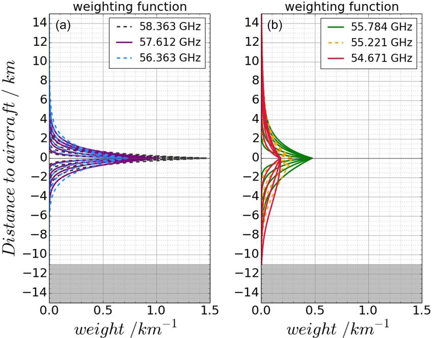
HALO MTP flight data cannot simply be calibrated by using quency channels are most sensitive to the air directly in front
fixed calibration parameters from laboratory measurements of the sensor (less than 2 km of distance; see Appendix or
at single arbitrary room temperatures, since such measure- Kenntner, 2018, for more details). Thus, the average HALO
ments are only representative of specific instrument states. TS value of the 13 s period it takes to record an entire MTP
Still, it is possible to apply a linear fit to the data by providing measurement cycle (with the 0◦ measurement being in the
a relationship between the MTP scanning unit temperature middle of the cycle) is representative of the air masses probed
https://doi.org/10.5194/amt-14-1689-2021 Atmos. Meas. Tech., 14, 1689–1713, 20211700 M. Heckl et al.: Measurement characteristics of an airborne microwave temperature profiler
Figure 8. Calibration parameters calculated from hot–cold calibration for standard frequency channels during cold-chamber measurements.
(a) Slope of calibration line. (b) Receiver noise temperature (TR ). (c) Calculated hot target TBs at different scanning unit temperatures during
cold-chamber measurements. Small dots: single measurements contributing to the average at one scanning unit temperature. Orange line:
Pt100 sensor readings.
the exact temperature of which is unknown. There are no
temperature sensors built into the absorber material, which
could be used to derive the thermal gradient, and measure-
ments with a thermal imager would require disassembling
of the instrument and are not an option. Still, to investigate
the hot target measurement characteristics, the calibration pa-
rameters determined from the hot–cold calibration method
are used to calculate the hot target TB associated with the
current measurement signal. Indeed, Fig. 8c shows the clear
trend towards colder TBs with lower scanning unit tempera-
tures, which correspond to a colder environment of the MTP
instrument, contrary to the readings of two Pt100 tempera-
Figure 9. Calculated ND offset temperature for occurring ND count ture sensors, which show the intended target temperature of
offsets (for better comparability, the means of the temperature and the heaters placed at the metal back of the target of just below
count values have been removed – mean values are shown in Ta- 45 ◦ C during entire mission flights (orange line in Fig. 8c).
ble 4). Color coding is as follows. For the MTP scanning unit tem- The difference can be as large as 3 K. However, the linearity
perature blue indicates colder and red warmer; black line: linear fit of the sensor again allows for a linear fit between the current
linking ND offset temperature to offset counts.
scanning unit temperature and the average associated hot tar-
get TB. Thus, in-flight calibration can be performed using a
corrected hot target TB, according to the MTP instrument’s
by the 0◦ elevation measurements. Hence, the calibration pa- housekeeping data. The parameters to correct the hot target
rameters can also be derived by combining the calibration TBs used in the calibration are shown in Table 5.
measurement while pointing at the hot target with the hori-
zontal measurement using Eq. (8a).
4.3 Comparison of calibration methods
4.2.3 Hot target temperature measurement
There are eight different ways to perform the calibration
The housekeeping data of the MTP indicate large tempera- calculations with and without applying the corrections dis-
ture differences of up to 55 K between the air in front of the cussed in the previous sections, as summarized in Table 6.
hot target and the heated back. Temperature gradients within All methods are compared to find the best practice of deriv-
the absorber material could lead to a misinterpretation of the ing TBs from MTP raw counts by applying all eight methods
measured brightness temperature, since the calibration mea- to the same set of mission data. To do so, segments from all
surement is mostly influenced by the front of the absorber, ML CIRRUS mission flights are used during which the alti-
Atmos. Meas. Tech., 14, 1689–1713, 2021 https://doi.org/10.5194/amt-14-1689-2021M. Heckl et al.: Measurement characteristics of an airborne microwave temperature profiler 1701
Table 4. Linear fit values linking the noise diode offset temperature
to MTP noise diode offset counts.
Lin fit slope
0.0647
0.0559
0.0922
10−6 K counts−2
LO Ref. cND Ref. TND Lin. fit slope
Table 3. Linear fit values linking calibration slope values and receiver noise temperature TR (calibration y intercept) to MTP scanning unit temperature and hot target counts. (GHz) (K) (K counts−1 )
56.363 2799 120.90706 0.033089
57.612 3049 123.43799 0.046590
58.363 2932 117.53960 0.052118
524.492
464.104
492.777
Ref TR
K counts−1
Table 5. Linear fit values used to correct the MTP hot target bright-
ness temperature.
Hot target counts chot
LO Ref. TSC Ref. Thot Lin. fit slope
Lin fit slope
2.0141
1.8964
3.4361
10−6 K counts−2
(GHz) (◦ C) (◦ C) (◦ C ◦ C−1 )
56.363 7.518 43.271843 0.89126
57.612 7.527 43.036542 0.103719
58.363 7.474 43.211868 0.088969
0.043154
0.040446
0.040031
Ref scal
K counts−1
tude of the aircraft did not change by more than 50 m during
a measurement cycle and no curves were flown (roll smaller
than 5◦ ). Note that this definition of usable segments is not
based on any parameters connected to the instrument state of
the HALO MTP (e.g., scanning unit temperature), leading to
counts
19486
19292
20213
Ref chot
the inclusion of measurement cycles with possibly unstable
measurement conditions, e.g., shortly after altitude changes.
The only exception is that only those segments are used, dur-
Lin. fit slope
0.3132
0.2716
0.4599
10−5 counts−1
ing which the ND did not show failures, to ensure compara-
bility of all calibration methods. This way, 38 flight segments
with at least a 10 min duration (i.e., including at least 50 mea-
surement cycles) could be identified. The TBs are calculated
based on each individual measurement cycle, but using the
calibration coefficients (scal and TR ) calculated from the av-
524.492
464.104
492.777
Ref. TR
K counts−1
erage of the relevant data from the seven previous cycles, the
seven following cycles, and the cycle itself (N = 15) to ac-
Scanning unit temperature
count for noise in the calibration measurement signals. As an
example, the resulting TBs of the 56.363 GHz measurements
at a 0◦ limb-viewing angle during one segment of ML CIR-
Lin. fit slope
1.0937
0.9989
1.7775
10−5 counts−1
RUS flight MLC10 on 11 April 2014 are shown in Fig. 10
(top panel). The TBs resulting from all calibration methods
show the same time-dependent variations and mainly differ
in their offset to HALO TS, indicating that differences in the
respective calibration coefficients affect the absolute accu-
racy of the derived TBs more than the precision.
0.043154
0.040446
0.040031
Ref. scal
K counts−1
To further investigate the precision of the MTP measure-
ments, a leg-mean value of the HALO TS and the TBs of the
0◦ elevation measurements is used to determine the offset,
which is subtracted from the TBs at all elevation angles:
◦C
7.518
7.527
7.474
Ref. TSC
TBcorr (νLO , α) = TB (νLO , α) − TB (νLO , 0◦ ) − TS ,
(9)
with TB (νLO , α) and TBcorr (νLO , α) denoting the original and
the corrected TBs under elevation angle α and at a specific
56.363
57.612
58.363
frequency channel (i.e., LO), respectively. TB (νLO , 0◦ ) de-
GHz
LO
notes the leg mean of the original TBs measured under 0◦
https://doi.org/10.5194/amt-14-1689-2021 Atmos. Meas. Tech., 14, 1689–1713, 2021You can also read