Surface flux estimates derived from UAS-based mole fraction measurements by means of a nocturnal boundary layer budget approach
←
→
Page content transcription
If your browser does not render page correctly, please read the page content below
Atmos. Meas. Tech., 13, 1671–1692, 2020
https://doi.org/10.5194/amt-13-1671-2020
© Author(s) 2020. This work is distributed under
the Creative Commons Attribution 4.0 License.

Surface flux estimates derived from UAS-based mole fraction
measurements by means of a nocturnal boundary layer budget
approach
Martin Kunz1 , Jost V. Lavric1 , Rainer Gasche2 , Christoph Gerbig1 , Richard H. Grant3 , Frank-Thomas Koch4 ,
Marcus Schumacher4,a , Benjamin Wolf2 , and Matthias Zeeman2
1 Max Planck Institute for Biogeochemistry, Jena, Germany
2 Instituteof Meteorology and Climate Research (IMK-IFU), Karlsruhe Institute of Technology,
Garmisch-Partenkirchen, Germany
3 Department of Agronomy, Purdue University, West Lafayette, IN, USA
4 Deutscher Wetterdienst, Meteorologisches Observatorium Hohenpeißenberg, Germany
a now at: Alfred Wegener Institute, Helmholtz Centre for Polar and Marine Research (AWI), Neumayer station III, Antarctica

Correspondence: Martin Kunz (mkunz@bgc-jena.mpg.de)

Received: 31 May 2019 – Discussion started: 27 August 2019
Revised: 17 February 2020 – Accepted: 19 February 2020 – Published: 6 April 2020

Abstract. The carbon exchange between ecosystems and the           1   Introduction
atmosphere has a large influence on the Earth system and
specifically on the climate. This exchange is therefore be-        The terrestrial biosphere plays a major role in the carbon cy-
ing studied intensively, often using the eddy covariance (EC)      cle. It has taken up approximately one-quarter of the car-
technique. EC measurements provide reliable results under          bon emitted by human activities since 1750 (Ciais et al.,
turbulent atmospheric conditions, but under calm and stable        2013), but the future development of this land sink under
conditions – as they often occur at night – these measure-         a changing climate is uncertain. Given its importance, the
ments are known to misrepresent exchange fluxes. Nocturnal         biosphere–atmosphere exchange is being studied intensively.
boundary layer (NBL) budgets can provide independent flux          On the ecosystem level, sources and sinks of carbon diox-
estimates under stable conditions, but their application so far    ide are commonly quantified using the eddy covariance (EC)
has been limited by rather high cost and practical difficulties.   technique (Baldocchi, 2003). During the day, when the air
Unmanned aircraft systems (UASs) equipped with trace gas           is turbulently mixed, the EC technique provides reliable di-
analysers have the potential to make this method more acces-       rect measurements of net ecosystem exchange (NEE). How-
sible. We present the methodology and results of a proof-of-       ever, EC measurements often misrepresent nighttime fluxes
concept study carried out during the ScaleX 2016 campaign.         (Goulden et al., 1996; Gu et al., 2005). This is related to the
Successive vertical profiles of carbon dioxide dry-air mole        stable stratification that often develops close to the surface at
fraction in the NBL were taken with a compact analyser car-        night. Stable conditions combined with low wind speeds vi-
ried by a UAS. We estimate an average carbon dioxide flux of       olate assumptions underlying the EC technique (see Aubinet
12 µmol m−2 s−1 , which is plausible for nocturnal respiration     et al., 2012, for a comprehensive discussion). Despite large
in this region in summer. Transport modelling suggests that        efforts, there is currently no generally accepted solution for
the NBL budgets represent an area on the order of 100 km2 .        how to obtain reliable measurements of nighttime fluxes us-
                                                                   ing the EC technique (Gu et al., 2005; Aubinet et al., 2010;
                                                                   Hayek et al., 2018).
                                                                      Daytime NEE consists of photosynthetic uptake and re-
                                                                   lease of carbon through respiration. Nighttime NEE is gov-
                                                                   erned by respiration only, as photosynthesis cannot take

Published by Copernicus Publications on behalf of the European Geosciences Union.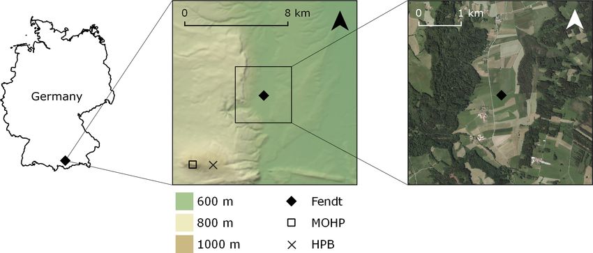
1672                         M. Kunz et al.: Surface flux estimates derived from UAS-based mole fraction measurements

place without light. Photosynthetic uptake and total respira-     to determine a budget by identifying an effective accumula-
tion fluxes are usually of the same order of magnitude, but       tion height from either heat flux or balloon-borne humidity
with opposite sign. Therefore, even slight underestimation        and temperature measurements and assuming a uniform ac-
of nocturnal respiration can result in a considerable over-       cumulation rate of CO2 up to this height. Winderlich et al.
estimation of an ecosystem’s long-term carbon uptake. Fur-        (2014) used CO2 and CH4 dry-air mole fraction measure-
thermore, daytime fluxes are often partitioned into photosyn-     ments at six heights on a 301 m tall tower, yielding profiles
thetic uptake and respiration using methods that rely on the      that encompass the whole NBL during most nights. Often
nighttime measurements (Falge et al., 2001; Reichstein et al.,    the NBL budget method is applied without a tower. A teth-
2005; Lasslop et al., 2010; Wohlfahrt and Galvagno, 2017).        ered balloon can lift a 100–300 m long hose through which a
Errors in the nocturnal fluxes might compromise this parti-       ground-based gas analyser samples air from different heights
tioning.                                                          (Choularton et al., 1995; Denmead et al., 1996; Culf et al.,
   The nighttime problem of EC measurements calls for error       1999). Alternatively, a light analyser can be carried by the
quantification and potentially correction. Ideally, this would    tethered balloon directly (Pattey et al., 2002).
be achieved by comparison to a method that is sensitive to           Despite providing unique information, the NBL budget
fluxes in the same area but is not based on the same assump-      method has been applied only infrequently in recent years.
tions as the EC technique. Unfortunately, no such method is       This might be related to the cost and operational limits of
available. Constraining the error of EC measurements must         towers and tethered balloons. Unmanned aircraft systems
therefore rely on methods that determine fluxes on smaller        (UASs) could make the NBL budget method more accessi-
and larger scales.                                                ble. UASs with payload capacities on the order of 1 kg are
   Enclosure-based methods and biometric approaches, in-          now available for a few thousand euros. When equipped with
cluding plant growth assessment and stock inventories, are        lightweight trace gas analysers and meteorological sensors
often employed to obtain independent estimates for NEE            (Kunz et al., 2018), they have the potential to probe the NBL
(Goulden et al., 1996; Wilson and Baldocchi, 2001; Campi-         with large flexibility at low cost. Multicopters are a particu-
oli et al., 2016). These methods quantify the exchange of car-    larly attractive type of UAS for this kind of study, because
bon on a much smaller spatial scale than EC measurements.         their vertical take-off, vertical landing and hovering capabil-
The chambers typically used for determining soil respiration      ity makes them easy to operate in a range of environments.
cover an area of less than 1 m2 , while the EC technique is          However, the air movement caused by a UAS can disturb
sensitive to fluxes from an area of 104 –106 m2 , depending on    the NBL and thereby compromise the measurements. A reli-
the site and on meteorological conditions (Chen et al., 2009).    able NBL budget can be determined only if this issue is ad-
Given these different scales, inhomogeneities in the ecosys-      dressed. A second challenge is not specific to UASs but com-
tem under study, such as spatial variability of soil proper-      mon to all NBL budgets: the area contributing to the budget
ties (e.g. texture, carbon content, nitrogen content), soil en-   depends heavily on the meteorological conditions and can
vironmental conditions (e.g. soil temperature and moisture)       extend far from the point of measurement. For a given time
or plant community composition, can lead to biases in the         and site this footprint cannot be influenced by experimental
comparison.                                                       design. Nevertheless, knowledge of the footprint is benefi-
   In order to counteract these biases, larger-scale flux es-     cial for the data analysis and interpretation of the results. In
timates should be obtained in addition to enclosure-based         earlier NBL studies, this topic received only basic treatment
or biometric measurements when constraining the error of          (Culf et al., 1999) or was ignored altogether.
EC measurements. Nocturnal boundary layer (NBL) bud-                 To assess the suitability of UASs as measurement plat-
gets, first described by Choularton et al. (1995) and Den-        forms for the creation of NBL budgets, we carried out a
mead et al. (1996), provide such estimates. The NBL budget        proof-of-concept study. We deployed a carbon dioxide anal-
method makes use of the stable stratification at night, which     yser on a multicopter and repeatedly sampled vertical pro-
can act as a flux-integrating enclosure. During clear nights,     files of the NBL during two nights in July 2016 as part of
the emission of thermal radiation cools down the Earth’s sur-     the ScaleX 2016 campaign in Fendt, Germany. Section 2 is
face much faster than the air, owing to the surface’s higher      a description of the site and the available ground-based in-
emissivity. An inversion layer forms, inhibiting exchange of      strumentation, the airborne measurement system and the un-
air between the stable NBL and the neutral residual layer         manned aircraft. In Sect. 3 we explain how we dealt with
above (Stull, 1988). Any tracer emitted from the surface into     the disturbance caused by the UAS, which post-processing
the atmosphere is therefore accumulated within the NBL. By        steps we carried out and how we determined the NBL bud-
measuring the rate of accumulation, the tracer flux can be        get. Furthermore, we delineate how a Lagrangian transport
estimated.                                                        model can be applied to identify the areas that contributed to
   Different setups have been used for NBL budgeting.             the budget, i.e. how to determine the footprint of our flux es-
Acevedo et al. (2004) measured CO2 dry-air mole fractions         timates. In Sect. 4 we present and discuss the profiles taken
at a 12 m tower, sampling only the lowest parts of the NBL.       by the UAS, the fluxes obtained from the NBL budget and
Although they did not sample the whole layer, they were able      a summary of the footprint analysis. We compare our obser-

Atmos. Meas. Tech., 13, 1671–1692, 2020                                             www.atmos-meas-tech.net/13/1671/2020/
M. Kunz et al.: Surface flux estimates derived from UAS-based mole fraction measurements 1673
vations to references and assess the robustness of our flux mast. Each inlet was sampled once every 7.5 min, with oc-
calculation. In Sect. 5 we summarise the merits and experi- casional interruptions due to calibrations and other measure-
mental challenges of our approach. ments. An EC system installed at 3.5 m height (Zeeman et al.,
2017) quantified the turbulent exchange of CO2 . Air temper-
ature as well as upward and downward radiation were mea-
2 Site and instrumentation sured at 2 m height. Two sets of automated chambers were
operated to determine the total NEE or respiration flux of
2.1 Fendt site
grass and soil. One set comprised four LI-8100 long-term
The Fendt site is located in southern Germany in the Alpine chambers (LI-COR, Lincoln, NE, USA), two with a clear
Foreland (Fig. 1) at 47.833◦ N, 11.060◦ E (WGS84), 600 m enclosure for measuring NEE and two with an opaque en-
above mean sea level. closure for measuring respiration (Zhao et al., 2018). All
The site lies in a flat valley bordered by a gentle slope to four chambers covered an area of 317.8 cm2 and will be re-
the east and a steep slope leading to a 100 m higher plateau to ferred to as “small chambers” from here on. The other set
the west. The valley floor is dominated by pasture and some consisted of five custom-built opaque chambers covering an
crops, predominantly maize, which in Germany is typically area of 2500 cm2 , referred to as “big chambers” hereafter. All
sown in April or May and harvested between September and the instruments mentioned so far were located close to each
November. The slopes to the east and west are covered with other, and the horizontal distance between any of the instru-
coniferous and mixed forest, respectively. Fendt belongs to ments and our UAS was always smaller than 200 m during
the district Weilheim–Schongau, which has a population den- the flights.
sity of 139 km−2 (Statistisches Bundesamt , Destatis, 35th Besides the on-site instruments, we use two more data
percentile of all districts in Germany). sources for our analysis. One is the observation of cloudi-
While soil identification at the Fendt site resulted in Stag- ness at the Meteorological Observatory Hohenpeißenberg,
nosols at three locations, soil organic carbon (SOC) content recorded every hour either by a person or an automated in-
was determined additionally at 20 locations within a regu- strument. We consider these 5 km distant measurements rep-
lar grid covering an area of 300 m by 300 m. SOC content resentative for Fendt, with a potential time lag on the order of
at 5 cm depth varied between 4 % and 11 %, while at 50 cm 1 h in the case of synoptic events. The second non-local data
depth, values of up to 23 % were obtained. The highest SOC source is the greenhouse gas monitoring system at the ICOS
contents were observed at the eastern side of the regular grid station Hohenpeißenberg, situated at 934 m above mean sea
where a peat area is located. According to BGR (2013), or- level. We use its measurements of the CO2 dry-air mole frac-
ganically rich soils (Cambisols and Histosols) prevail within tion at 131 m height above ground level, i.e. at 460 m above
a 20 km radius around the Fendt site (Fig. 2a). The dominant the Fendt site.
land cover in this region includes crops, pasture and forest
2.3 Airborne payload
(Fig. 2b).
About 5 km south-west of the Fendt site lies an isolated, For the study presented here, temperature, pressure, relative
988 m high mountain, the “Hoher Peißenberg”. Close to humidity and CO2 dry-air mole fraction of ambient air were
its summit the German Weather Service (Deutscher Wet- measured using COCAP, the COmpact Carbon dioxide anal-
terdienst, DWD) operates the Meteorological Observatory yser for Airborne Platforms, developed at the Max Planck In-
Hohenpeißenberg (MOHP) and the ICOS (Integrated Car- stitute for Biogeochemistry in Jena (see Kunz et al., 2018, for
bon Observation System) station Hohenpeißenberg (HPB, a detailed description). COCAP was mounted below the mul-
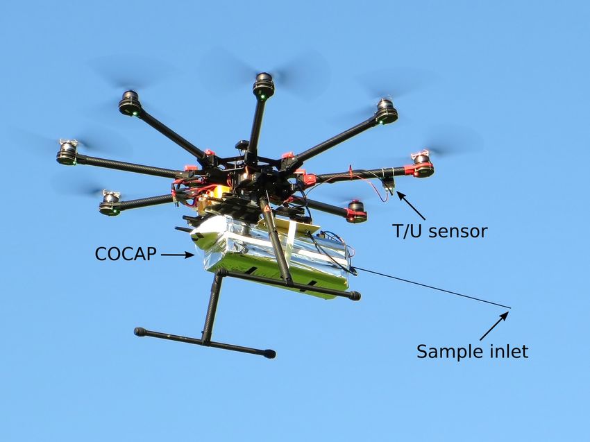
Fig. 1). ticopter. Air samples for the measurement of carbon dioxide
dry-air mole fraction were drawn from an inlet placed 30 cm
2.2 Ground-based instrumentation
below and 20 cm to the side of the rotors (Fig. 3).
Fendt is part of the TERENO (Terrestrial Environmental Ob- The temperature and humidity sensor board, requiring
servatories) network and is extensively instrumented for the strong ventilation for the fastest response, was placed directly
purpose of long-term monitoring of land–atmosphere ex- below one of the rotors. The sensor for ambient pressure
change (Mauder et al., 2013; Kiese et al., 2018). Comple- was located inside COCAP’s housing, which was not her-
mentary observations were made during the ScaleX 2016 metically sealed and therefore in equilibrium with ambient
campaign (Wolf et al., 2017). In the following, we list only pressure.
those instruments that produced the data presented in this The measurement principles employed by the different
publication. sensors as well as their measurement uncertainties are listed
During the ScaleX 2016 campaign, CO2 dry-air mole frac- in Table 1. The uncertainty of the calibration is included in
tion at heights of 1, 3 and 9 m above ground level was mea- the measurement uncertainties reported.
sured with a cavity ring-down spectrometer by successive
sampling of air through three inlets installed at a 9 m high
www.atmos-meas-tech.net/13/1671/2020/ Atmos. Meas. Tech., 13, 1671–1692, 2020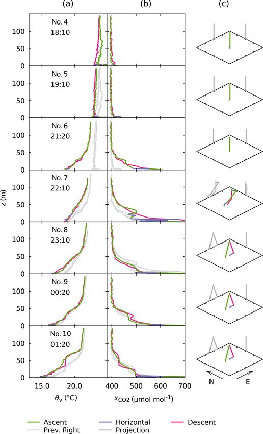
1674                         M. Kunz et al.: Surface flux estimates derived from UAS-based mole fraction measurements

Figure 1. Location, topography and aerial image of the Fendt site and its surroundings. MOHP is the Meteorological Observatory Hohen-
peißenberg, and HPB is the ICOS station Hohenpeißenberg. Digital elevation model and aerial imagery by Bayerische Vermessungsverwal-
tung, https://www.geodaten.bayern.de (last access: 25 March 2020).

Figure 2. (a) Soil types in the region around the Fendt site, based on BGR (2013), denoted in WRB classification (IUSS Working Group
WRB, 2015). “Fl./Gl.” stands for “Fluvisols/Gleysols”. (b) Simplified land cover map (CORINE 2012 v18.5, European Environment Agency,
EEA, 2016) of the same region. In both panels the location of the Fendt site is marked with a black diamond.

2.4    Unmanned aircraft                                             exceeded 5 kg, all flights were limited to a maximum height
                                                                     of 150 m.

During ScaleX 2016 COCAP was deployed on an S1000                    3     Methods
multicopter (SZ DJI Technology, China) controlled by a Pix-
hawk autopilot (3D Robotics, Berkeley, CA, USA) running              3.1    Disturbance by the UAS
the Ardupilot APM:Copter v.3.3.3 firmware. Take-off mass
of the whole system was 8 kg. The multicopter was pow-               A multicopter as a rotary-wing aircraft counterbalances grav-
ered by three lithium polymer batteries with a voltage of            ity by accelerating air downwards through the movement of
22.2 V and a capacity of 5000 mAh each, achieving a maxi-            its rotors. The resulting displacement of air can interfere with
mum flight time of 12 min. Our special flight permit included        in situ measurements, because air might be sampled at a lo-
nighttime flights, but because the take-off mass of our UAS          cation where it would normally not reside. In addition, vol-

Atmos. Meas. Tech., 13, 1671–1692, 2020                                                www.atmos-meas-tech.net/13/1671/2020/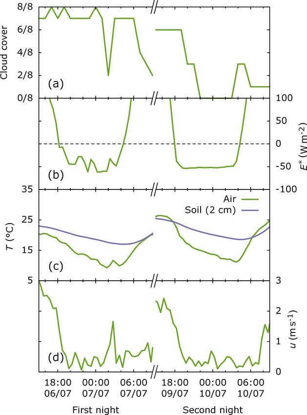
M. Kunz et al.: Surface flux estimates derived from UAS-based mole fraction measurements                                          1675

Table 1. Measurement principles, uncertainties and calibration range of the airborne sensors.

                                 CO2 dry-air mole fraction    Temperature            Pressure         Humidity
                  Principle      nondispersive infrared       platinum resistance    piezoresistive   capacitive polymer
                  Uncertainty    see Sect. 4.1                0.15 ◦ C               1.5 hPa          2%
                  Cal. range     380–600 µmol µmol−1          0–30 ◦ C               400–1000 hPa     20 %–90 %

                                                                        ondly, in our nighttime experiments the air near the ground
                                                                        is stably stratified. Therefore, air pushed downwards by the
                                                                        rotors experiences a restoring upward force, increasing the
                                                                        chance that closed flow loops form. Thirdly, the strongest
                                                                        gradients in temperature and CO2 dry-air mole fraction are
                                                                        present close to the ground, hence even a small displacement
                                                                        of air can have a large effect on the measured values.
                                                                           In the case of considerable horizontal air speed, due to
                                                                        either wind or horizontal flight, the rotor-induced airflow
                                                                        should have a smaller effect on measurements because the
                                                                        sampling system is moving away from air that has been dis-
                                                                        placed. We investigated this effect by flying horizontally at
                                                                        different speeds over a homogeneous meadow (see Sect. 4.4).
                                                                           Based on the considerations above and the data presented
                                                                        in Sect. 4.3 and 4.4, we determine the NBL budget only
                                                                        from those measurements that were taken during ascent of
Figure 3. COCAP was carried by a multicopter during the                 the multicopter. The sensitivity of the NBL-derived fluxes to
ScaleX 2016 campaign. The positions of the sample inlet for the         inclusion of hover and descent data is discussed in Sect. 4.5.
CO2 measurement and of the temperature and humidity sensor
                                                                        Furthermore we discard COCAP’s xCO2 data collected below
board are indicated.
                                                                        9 m height for the calculation of the NBL budget. Instead,
                                                                        the lowest part of the xCO2 profile is defined by the stationary
                                                                        measurements at the 9 m mast at 1, 3 and 9 m height. Pressure
umes of air originating from different locations can be mixed
                                                                        and temperature at these levels are interpolated from CO-
together. The greater the displacement and mixing caused by
                                                                        CAP’s measurements. During flight, the horizontal distance
the UAS, the greater the potential impact on the measure-
                                                                        between COCAP and the 9 m mast was less than 150 m at any
ment of a gradient, for example. Air movement below and
                                                                        time. Hence, we do not expect pronounced horizontal gradi-
above the rotors is not symmetric: below a rotor, air is pushed
                                                                        ents in xCO2 between the measurement locations. In Sect. 4.6
downwards as a directed stream with high speed. In contrast,
                                                                        we discuss how the NBL-derived fluxes are affected if the
the air flow towards the rotor comes from different directions
                                                                        data from the 9 m mast are not used.
and has a lower speed. The reader can easily confirm this
with a fan or a hair dryer: while the outflow of air can be felt        3.2    Correction for response time of sensors
metres away, the inflow is hard to sense even near the rotor.
   In view of the asymmetric flow pattern, we expect that dur-          On a moving platform the finite response time of sensors can
ing ascent of the UAS air parcels are measured with negli-              be a source of measurement error, as the response time dis-
gible displacement from their undisturbed location. During              torts the attribution of data points to time and location. CO-
descent, however, the sensors are moved into a volume that              CAP’s pressure and temperature sensors are fast enough for
potentially has been flushed with air originating from sev-             this effect to be neglected, but both the humidity and the CO2
eral metres above. During hovering at a fixed location or dur-          sensor require correction.
ing purely horizontal movement, the sensors might reside in                The response of a capacitive humidity sensor can be ex-
a partially closed flow loop that extends below and to the              pressed following Miloshevich et al. (2004):
side of the multicopter, effectively measuring a mixture of
                                                                         dUm
air from different locations.                                                = k(Ua − Um ).                                         (1)
   For the study presented here, flying near the ground can               dt
have a particularly strong influence on the measurements for            Ua and Um are ambient and measured relative humidity, re-
three reasons. Firstly, downward motion of the air stops at             spectively. The coefficient k is inversely related to the sen-
the ground and displaced air must move laterally or upwards,            sor’s response time and might be temperature-dependent.
making a fast flow path back to the UAS more likely. Sec-               Solving Eq. (1) for Ua provides a simple way to compute

www.atmos-meas-tech.net/13/1671/2020/                                                      Atmos. Meas. Tech., 13, 1671–1692, 2020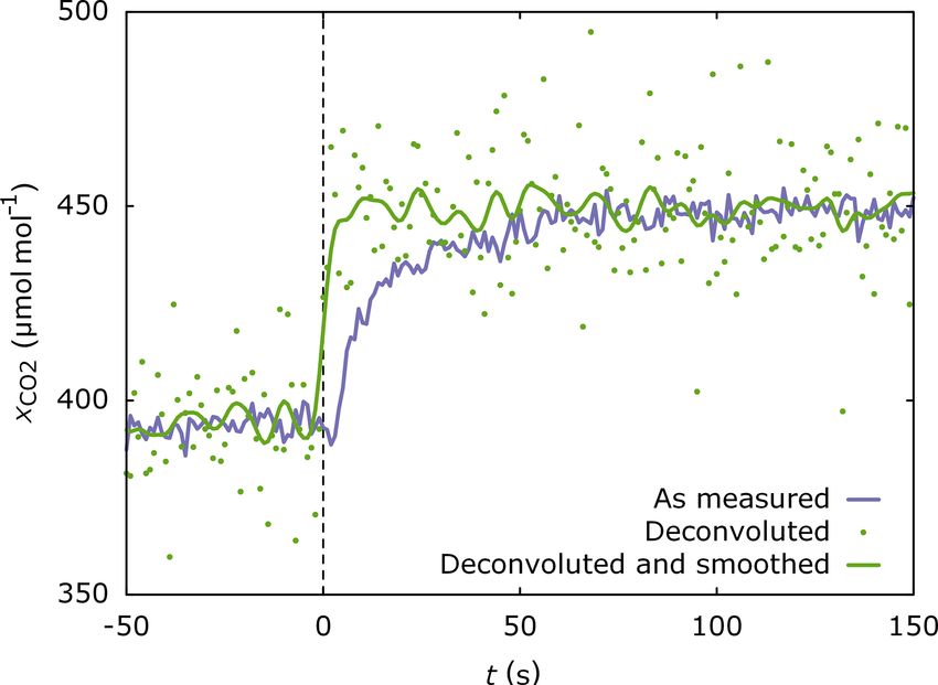
1676 M. Kunz et al.: Surface flux estimates derived from UAS-based mole fraction measurements
true humidity from measurements. We use a fourth-order
Savitzky–Golay filter (Savitzky and Golay, 1964) with a
length of 15 samples to compute dU m
dt while keeping high-
frequency noise at an acceptable level. The coefficient k =
14 s was determined by an optimisation that minimises the
difference between the corrected humidity profiles for ascent
and descent. We tested a linear and quadratic dependence of
k on ambient temperature, but we found no improvement that
would justify the additional degrees of freedom in the model.
The response of COCAP’s CO2 sensor is more complex.
Its response to step changes in CO2 dry-air mole fraction can
be approximated as
x0 if t < td
xSC (t) = (2)
a(x0 − x∞ )e(td −t)/τ1 + (1 − a)
Figure 4. Response of COCAP to an abrupt change in CO2 dry-air
(t
·(x0 − x∞ )e d −t)/τ 2 +x if t ≥ td .
∞ mole fraction xCO2 at the inlet at time t = 0 s. The measured signal
reveals a dead time of 5 s of the sampling system. Furthermore, the
Here x0 and x∞ denote the CO2 dry-air mole fraction before
step change in xCO2 is smoothed out. Both effects are removed by
and infinitely long after the step change, respectively, and td deconvolution at the cost of higher noise. Smoothing the deconvo-
is the sensor’s dead time. luted signal reduces the noise with only minor impact on the time
We determined the coefficient a, the dead time td , and the response. Smoothing was carried out by convolution with a Gaus-
time constants τ1 and τ2 from experimental data collected sian function of 5 s full width at half maximum (FWHM).
in the field. With COCAP running in flight configuration,
i.e. with the inlet tube attached, we connected a tube with
gas flowing from a cylinder. We observed a dead time of 3.3 Calculation of the NBL budget
td = 5 s between making the connection and the first change
of COCAP’s reading. The remaining parameters were found For a parcel of air in the atmosphere the following continuity
by least-squares regression of Eq. (2) to the data, yielding equation holds (Leuning, 2004, Eq. 6.2):
τ1 = 27 s and τ2 = 3.2 s.
∂c
Ignoring noise and calibration error, any CO2 signal xa is σ= + ∇ · (cu), (5)
reported by COCAP as the convolution of xa with the CO2 ∂t
sensor’s instrument function f (see Kunz et al., 2018): ∂c ∂c ∂c ∂c
= + c(∇ · u) + u +v +w . (6)
∂t ∂x ∂y ∂z
xm (t) = (xa · f )(t) (3)
Here σ is the strength of a volume source (or sink) of car-
with bon dioxide (µmol m−3 s−1 ), c is the concentration of carbon
dioxide and t denotes time. The components u, v and w of
0 if t < td the wind vector u point towards east (x direction1 ), towards
f= 1 dxSC (4)
x∞ −x0 · dt if t ≥ td . north (y direction) and upwards (z direction), respectively.
Molecular diffusion is neglected. Due to continuity of the air
As xSC is known from experiments, f can be calculated. The flow, the term c(∇ · u) equals zero. If we follow an air parcel
ambient signal xa can be recovered from the measured signal as it is transported by horizontal winds, those terms that con-
xm by deconvolution (Fig. 4). We carried out the deconvolu- tain a horizontal wind component vanish as well and Eq. (6)
tion in Fourier space where it is equal to a division. In the is reduced to
numerical implementation it is important to discretise f in a
way that does not underestimate the slope of f between the ∂c ∂c
σ= +w . (7)
time steps td and td + 1t, because doing so would lead to a ∂t ∂z
strong enhancement of the noise during the deconvolution of
Now we integrate vertically over those air parcels that form a
xm with f . The opposite error, i.e. overestimating the slope
vertical column over our site at the time of measurement (at
between td and td + 1t, is less critical and just results in a
earlier or later points in time, the air parcels are not aligned
slight smoothing.
in a vertical column, unless the wind vector is equal at all
1 Only here and in Eq. (6) x does denote a coordinate in space.
Elsewhere in this publication x denotes the dry-air mole fraction of
a substance.
Atmos. Meas. Tech., 13, 1671–1692, 2020 www.atmos-meas-tech.net/13/1671/2020/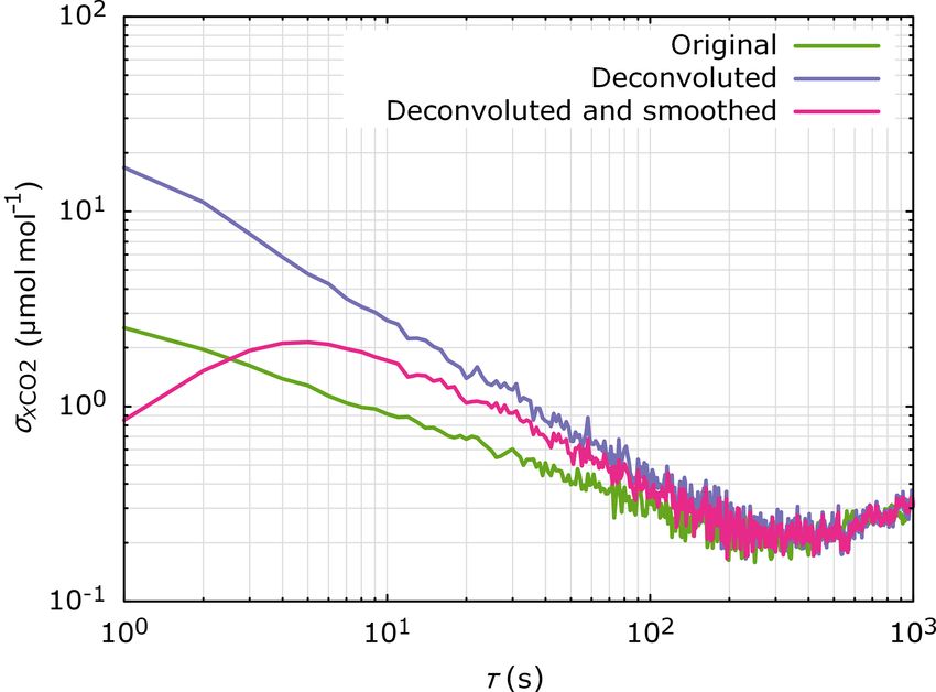
M. Kunz et al.: Surface flux estimates derived from UAS-based mole fraction measurements 1677
heights): Note that this is a weaker assumption than the horizontal
homogeneity of the CO2 concentration in the NBL presumed
Zzt Zzt Zzt in other studies (Choularton et al., 1995; Culf et al., 1999;
∂c ∂c
σ dz = S = dz + w dz . (8) Acevedo et al., 2004). All natural environments exhibit a cer-
∂t ∂z
0 0 0 tain horizontal heterogeneity in S. Daytime and nighttime
CO2 flux of a vegetated area are usually of the same order
For our measurements, we choose zt = 125 m, so all biotic
of magnitude, although different in sign. Before t0 , the con-
sources of carbon dioxide are within the column and S rep-
vective boundary layer is well mixed up to a height of typi-
resents NEE.
cally 1 km, whereas after t0 a strong NBL confines emissions
Between a reference time t0 (see below) and the time of a
from the surface to the lowest ≈ 100 m of the atmosphere
flight tF the column has accumulated
(see Sect. 4.3). Therefore, the horizontal heterogeneity in c
ZtF ZtF Zzt ZtF Zzt caused by the horizontal heterogeneity in S is 1 order of mag-
∂c ∂c nitude smaller during the day than during the night. The con-
Sdt = dzdt + w dzdt, (9)
∂t ∂z vective mixing during the day also keeps vertical gradients
t0 t0 0 t0 0
inside the boundary layer low; hence the approximation of
Zzt Zzt ZtF Zzt xCO2 (t0 ) being independent of z is justified.
∂c
= c(z, tF )dz − c(z, t0 )dz + w dzdt . Term B in Eq. (11) contains the product w ∂c/∂z, which
∂z
0 0 t0 0 generally includes both turbulent exchange and subsidence.
(10) However, when a stable NBL has developed, little turbulent
exchange takes place across the top of the NBL. In the stat-
Dividing the accumulated amount of CO2 by tF − t0 yields ically neutral residual layer above the NBL, turbulence is
NEE averaged over this time span, denoted S: present, but the vertical concentration gradient in the residual
layer and as a consequence the net vertical transport of CO2
Z tF Z zt Z zt
Sdt is small. Hence, we neglect turbulent exchange and iden-
c(z, tF )dz − c(z, t0 )dz
t0 0 0 tify w ∂c/∂z with subsidence or lifting. The vertical wind
tF − t0 = S = tF − t0 speed w due to subsidence at a height of 100 m is usually
(A) on the order of 100 m d−1 , i.e. very low and therefore chal-
lenging to measure. We retrieve an estimate of w from the
Z tF Z zt ∂c Integrated Forecast System (IFS) run by the European Cen-
wdzdt
t0 0 ∂z tre for Medium-Range Weather Forecasts (ECMWF).
+ tF − t0 .
In order to calculate ∂c/∂z at different times between t0
(B) and tF , we use a simple model for the growth of the NBL:
(11)
tF − t0
xCO2 (t, z) = xCO2 tF , z (t0 < t ≤ tF ) . (13)
Term A represents the enhancement in CO2 concentration t − t0
and term B the vertical exchange of CO2 . We choose t0 as the
time when the surface radiation balance becomes negative, Where tt−tF −t0
0
z exceeds the maximum height of the profile
i.e. the time when the stable NBL starts to form. A positive S measured at time tF , we assume the CO2 dry-air mole frac-
means emission of CO2 from the surface into the atmosphere. tion to be equal to xCO2 (t0 ). This model for the growth of the
The CO2 concentration c can be calculated from CO2 dry- NBL can be visualised best by starting at tF and looking back
air mole fraction xCO2 , air temperature T and dry pressure in time. At t = tF the factor (tF − t0 )/(t − tF ) is equal to unity
pd using the ideal gas constant R (Foken et al., 2012, p. 5): and the model yields the measured profile. At earlier times,
pd the measured profile is compressed in the z direction, such
c= xCO2 . (12) that the height of the NBL decreases linearly as we go back
RT in time. As t approaches t0 , the model yields a thin layer en-
As COCAP Rmeasures xCO2 , T , p and relative humidity U , riched with CO2 at the surface and a constant CO2 dry-air
z
the integral 0 t c(z, tF )dz in Eq. (11) term A is readily com- mole fraction of xCO2 (t0 ) above.
puted. However, each air parcel is sampled only once, at the The concentration c(t, z) is calculated from xCO2 (t, z) us-
time tF when it passes the FendtR z site. In order to evaluate the ing Eq. (12). To this end, we determine pd (t, z) and T (t, z)
second integral in term A, 0 t c(z, t0 )dz, we assume horizon- by linear interpolation in time between the first profile of the
tal and vertical homogeneity of the CO2 dry-air mole fraction night and the profile measured at tF .
at the time t0 ; i.e. xCO2 (t0 ) is assumed to be constant within In summary, the model for the growth of the NBL
the spatial domain relevant for our experiments. Thus we can represents four simplifying assumptions: (1) during the
calculate the second integral from the measurement of a dif- night,
R zt the NBL height increases linearly; (2) the integral
ferent column at Fendt at t0 . 0 CO2 (t, z)dz increases linearly with time; (3) the shape of
x
www.atmos-meas-tech.net/13/1671/2020/ Atmos. Meas. Tech., 13, 1671–1692, 2020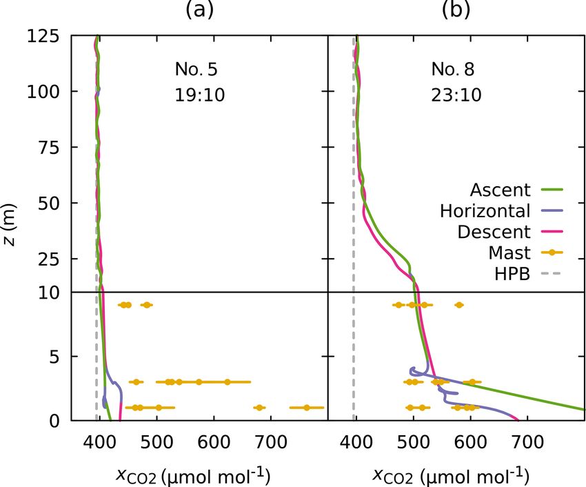
1678                           M. Kunz et al.: Surface flux estimates derived from UAS-based mole fraction measurements

the xCO2 profile within the NBL remains the same throughout            Eq. (11) term A and Eq. (12):
the night; and (4) the dry pressure and temperature of an air
column measured at Fendt are representative for the whole                                    Zzt
                                                                                                   pd (z, t)
footprint of the measurement (see Sect. 3.4).                                                                · f (z, t|lG1 , lG2 )dz
                                                                                                   RT (z, t)
                                                                                             0
                                                                       fF (t|lG1 , lG2 ) =                                             .   (14)
3.4    Footprint calculation                                                                                  t − t0
                                                                       Dry pressure pd and air temperature T at time t and height
The columns of air probed at Fendt at different times had              z are inter- or extrapolated from the measured profiles. The
a different history, depending on the wind field and atmo-             ensemble of mole fraction footprints comprises footprints for
spheric stability. Atmospheric transport models can identify           12 different measurement heights between 10 and 120 m in
the surface areas that have contributed to an observed tracer          10 m steps.
concentration, i.e. the footprint of an observation. We simu-             The meteorological data we use have a horizontal reso-
late atmospheric transport with STILT, the Stochastic Time-            lution of 0.1◦ × 0.1◦ , corresponding to 11 km × 8 km at the
Inverted Lagrangian Transport model (Lin et al., 2003; Ger-            latitude of Fendt. Terrain features that are smaller than a grid
big et al., 2003a), which is based on NOAA’s HYSPLIT par-              cell, like the valley slope to the west of the Fendt site, cannot
ticle dispersion model (Stein et al., 2015). In our configura-         be represented at these resolutions. The vertical resolution
tion, STILT launches 10 000 air parcels at different heights           of the meteorological data depends on height above ground.
(see below) at every full hour during the period of our NBL            The lowest layer extends from the ground to 10 m height, and
measurements. Driven by meteorological data with a resolu-             the following five layers extend from the top of the previous
tion of 0.1◦ × 0.1◦ from the ECMWF IFS (European Cen-                  layer to 31, 55, 80, 108 and 138 m. The temporal resolution
tre for Medium-Range Weather Forecasts Integrated Fore-                of the ECMWF IFS data is 3 h.
cast System), STILT calculates the back trajectories of these
parcels until 10 h in the past. For each time step of the sim-
ulated transport, the model determines the sensitivity of the          4     Results and discussion
CO2 concentration in the parcel to the CO2 flux at the sur-
                                                                       4.1    Uncertainty of xCO2 measurements
face. To do so, the height up to which mixing occurs is
estimated from the meteorological data using a modified                The uncertainty of COCAP’s xCO2 measurements due to drift
Richardson number method (Lin et al., 2003). Surface fluxes            and calibration errors is about 1 µmol mol−1 (Kunz et al.,
influence air parcels within a column that extends from the            2018). The additional uncertainty caused by noise is depen-
surface to one-half this height in each time step (Gerbig et al.,      dent on the data treatment, as can be seen from Fig. 5. This
2003b).                                                                Allan deviation plot (Allan, 1987) is based on measurements
   The back trajectories calculated by STILT are then aggre-           of a gas standard (xCO2 = 447.44 µmol · mol−1 ) over a period
gated into mole fraction footprints on a regular grid with a           of 1.4 h, taken in the field on 6 July 2016.
resolution of 2 km × 2 km. As explained in the previous sec-              The curves illustrate that deconvolution amplifies noise in
tion, we assume the xCO2 distribution to be homogeneous in             the data by a factor of 7 if no averaging is applied (τ = 1 s).
the lateral and horizontal directions at time t0 . We therefore        However, if more than 100 samples are averaged (τ ≥ 100 s),
restrict the aggregation to that part of each back trajectory          the difference between original and deconvoluted data be-
that lies between t0 and the time of measurement.                      comes negligible and the uncertainty of the average due to
   A single STILT run determines the sensitivity of an ob-             noise is lower than 0.5 µmol mol−1 . All our column integrals
servation at a specific height to upwind fluxes. Formally, the         (see Sect. 3.3) have a sample size larger than 100.
mole fraction footprint of a measurement taken at the ge-                 Figure 5 also shows that the Allan deviation of decon-
ographic location (l1 , l2 ) at time t and observation height          voluted data that have been smoothed by convolution with
z can be written as f (l1 , l2 , z, t | lG1 , lG2 ). As all our mea-   a Gaussian function of 10 s full width at half maximum
surements were taken at the same horizontal location, the              (FWHM) increases between τ = 1 s and τ = 5 s. This in-
dependency of f on l1 and l2 will be omitted hereafter.                crease is an artefact caused by the autocorrelation that the
The mole fraction footprint is a function whose value is               smoothing induces. If COCAP were perfectly calibrated and
the sensitivity to the surface flux at the grid cell specified         exhibited no drift, any single point in the smoothed data set
by (lG1 , lG2 ) in units of [f ] = µmol mol−1 µmol−1 m2 s. To          would have an uncertainty of 2.1 µmol mol−1 (corresponding
determine the relative contribution of surface fluxes in dif-          to τ = 5 s), not 0.8 µmol mol−1 (corresponding to τ = 1 s).
ferent areas to our NBL-derived fluxes, we need a differ-
ent but related function, the flux footprint fF with units             4.2    Meteorological conditions
[fF ] = µmol m−2 s−1 µmol−1 m2 s = 1. The flux footprint is
calculated by integration over an array of mole fraction foot-         From the data collected during ScaleX 2016 we calculate
prints for different measurement heights, i.e. analogous to            NEE for the nights 6–7 July and 9–10 July. The sun set at

Atmos. Meas. Tech., 13, 1671–1692, 2020                                                      www.atmos-meas-tech.net/13/1671/2020/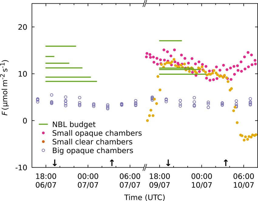
M. Kunz et al.: Surface flux estimates derived from UAS-based mole fraction measurements 1679
Figure 5. Allan deviation of CO2 dry-air mole fraction σxCO2 as
measured after deconvolution and after deconvolution followed by
smoothing (convolution with a Gaussian function of 5 s FWHM) for
different averaging periods τ . All three cases converge for averaging
periods longer than 100 s.
19:15 and 19:14 UTC on 6 and 9 July, respectively, and rose
at 03:25 and 03:27 UTC on 7 and 10 July, respectively. Both
nights were free of precipitation. Cloud cover was high dur-
ing the first night (see Fig. 6a), but the pronounced negative
net radiation (Fig. 6b) indicates that the clouds were mostly Figure 6. Meteorological conditions during the NBL soundings:
transparent for outgoing long-wave radiation. (a) cloud cover, (b) net radiation E ∗ , (c) temperature T of air
On the second night the sky was clearer, resulting in a (2 m height) and soil (2 cm depth), and (d) horizontal wind speed
steadier radiation balance. During both nights, strong radia- u (3.5 m height). Cloud cover was determined at MOHP, and all
tive cooling was observed. Air temperature decreased from other observations were made directly at Fendt. Time is given in
18 to 9 ◦ C and from 24 to 11 ◦ C over the course of the first Coordinated Universal Time.
and second nights, respectively (Fig. 6c). In combination
with low wind speeds (Fig. 6d) this led to the development of
a pronounced temperature inversion at the surface, i.e. a sta- The times given in Figs. 7 and 8 are the midtimes of the
ble NBL. The change from positive to negative net radiation flights rounded to a full 10 min for readability. The exact
occurs approximately at t0 = 18:00 UTC on both nights. times of take-off and landing are provided in Table 2.
During the first night, a stable NBL can be identified from
the UAS profiles for flights 6 through 10. The upper end of
4.3 Profiles the temperature inversion aligns with the top of the CO2 en-
hancement to within 10–20 m. At the time of flights 6 and
We carried out a total of 27 flights during the ScaleX 2016 8 through 10, the NBL has a height of 50–70 m, whereas
campaign. For the calculation of a NBL budget, we anal- the profile from flight 7 indicates a greater NBL height of
yse those flights that took place after t0 = 18:00 UTC and ≈ 100 m. We interpret this as an indication that the column
reached a height of at least 125 m. Twelve flights fulfil these measured in flight 7 has been influenced by katabatic inflow
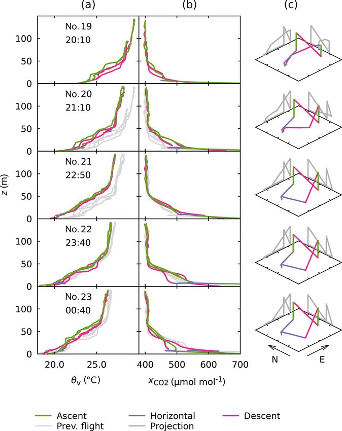
criteria: flights 4 through 10 (first night, Fig. 7) and flights 19 of cool, CO2 -enriched air at some point during the night, po-
through 23 (second night, Fig. 8). For display in panel (b) of tentially hours before the flight and kilometres away from
Fig. 7 and 8 the CO2 dry-air mole fraction has been smoothed Fendt. This interpretation is supported by the flux estimates
with a Gaussian filter of 5 s FWHM. To prevent distortion in (see Sect. 4.5). The profiles from flight 5, which exhibit vir-
the vertical direction, the height above ground level z has tually no gradient, are discussed below.
been filtered the same way. For this reason, the upper end of During the second night, a stable NBL with a height of 50–
the profiles in panel (b) is at a slightly lower height than in 70 m is visible in all profiles. The flight pattern had been re-
panel (a). Calculation of the NBL fluxes (see Sect. 4.5) was fined and included two ascents and descents far enough from
carried out with unfiltered xCO2 and z. each other to avoid disturbance of the measurements in the
www.atmos-meas-tech.net/13/1671/2020/ Atmos. Meas. Tech., 13, 1671–1692, 2020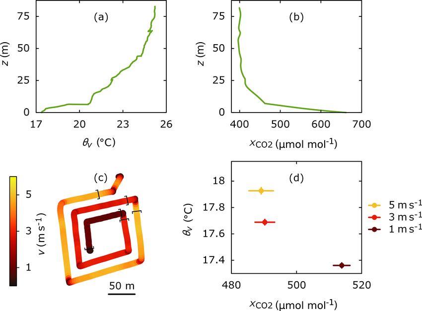
1680                          M. Kunz et al.: Surface flux estimates derived from UAS-based mole fraction measurements

Table 2. Take-off and landing times (UTC).

                               Flight   Date                      Take-off        Landing     Duration
                               no.      (year-month-day)     (hour:minute)   (hour:minute)
                               4        2016-07-06                   18:04           18:14    10 min 50 s
                               5        2016-07-06                   19:05           19:16    10 min 58 s
                               6        2016-07-06                   21:13           21:23    10 min 13 s
                               7        2016-07-06                   22:09           22:19    09 min 20 s
                               8        2016-07-06                   23:06           23:16    09 min 43 s
                               9        2016-07-07                   00:18           00:28    09 min 23 s
                               10       2016-07-07                   01:11           01:20    09 min 18 s
                               19       2016-07-09                   20:01           20:11    09 min 58 s
                               20       2016-07-09                   21:02           21:13    11 min 31 s
                               21       2016-07-09                   22:43           22:55    11 min 23 s
                               22       2016-07-09                   23:39           23:49    10 min 34 s
                               23       2016-07-10                   00:31           00:42    10 min 32 s

second part by air movements caused during the first part.             later analysis of flight 14 (see Sect. 3.1) revealed that the
These redundant measurements give insight into the reliabil-           ground speed was insufficient to fully reach this goal.
ity of the measurement system and the variability of temper-              The profiles for flight 5 are close to straight vertical lines,
ature and CO2 dry-air mole fraction on small temporal and              which would indicate a well-mixed atmosphere. However,
spatial scales. The data from flight 21 agree well between             they were measured under low wind speed 1 full hour after
each of the two ascents and descents, suggesting that distur-          the surface radiation balance became negative, i.e. under con-
bances by the UAS, instrument noise and drift are small com-           ditions favourable for the development of a stable nocturnal
pared to the observed signals. Flights 22 and 23 were carried          boundary layer and accumulation of CO2 near the ground.
out only 1 and 2 h later, respectively, and followed the same          This apparent contradiction can be explained by compar-
flight track. However, the data from these flights reveal con-         ing COCAP’s data to tower-based measurements. Figure 9a
siderable differences between each of the two ascents and de-          shows the CO2 profile taken by COCAP together with data
scents, especially in xCO2 for heights below 50 m. We inter-           from the 9 m mast and from HPB (see Sect. 2.1 and 2.2).
pret this as natural variability on the scale of the flight track,        The diagram includes those measurements from the mast
i.e. ≈ 200 m in horizontal distance and ≈ 3 min in time. This          that fall into the time interval from 15 min before take-off to
small-scale variability is a source of random error in NBL             15 min after landing. They reveal that the CO2 dry-air mole
budgets. In our flux calculations multiple ascents during the          fraction near the ground was increased relative to the upper
same flight are effectively averaged, resulting in a reduction         two-thirds of the profile and fluctuated strongly, e.g. between
of the random error.                                                   450 and 650 µmol mol−1 , at 3 m height. These observations
   The xCO2 profiles measured during flights 20, 22 and 23 all         are in line with a weakly stable layer near the surface: surface
exhibit a non-zero gradient with height in the region above            fluxes accumulated in this layer, but weak turbulent events
the strong inversion, indicating that some CO2 has escaped             caused by wind shear, for example, occasionally spread them
the stable NBL. This is supported by the profiles of virtual           out to higher layers. The disturbance by the multicopter dur-
potential temperature, which are more inclined above the               ing take-off or landing prevented COCAP from capturing
NBL in comparison to the first night. Both features might              this accumulation. On the other hand, the higher part of CO-
be the result of intermittent turbulence, a phenomenon often           CAP’s profile, taken in the residual layer that is left over from
observed at night that can have different causes (see Aubi-            the daytime mixed layer, matches the mean CO2 dry-air mole
net, 2008, and references therein). Our budgets include the            fraction measured at HPB during the time interval from 1 h
measurements up to 125 m height, so any CO2 that has been              before take-off to 1 h after landing. This agreement confirms
transported higher than this is missing in the budgets. In fu-         that COCAP was working properly during the flight.
ture campaigns, flights with a greater maximum height could               The profile from flight 8, carried out later in the same
be carried out to quantify the effect this has on the NBL-             night, is consistent with the measurements at the 9 m mast
derived fluxes, or to extend the budget vertically.                    (Fig. 9). We see two reasons for this difference to flight 5.
   The flight pattern used during the second night also in-            Firstly, the radiative cooling (see Fig. 6) at the time of flight 8
cluded two horizontal transects at 10 m height that were               (23:10) was stronger than at the time of flight 5 (19:10). The
flown at a ground speed of 3 m s−1 . Their purpose was to en-          temperature gradient near the ground was not resolved dur-
able measurements of undisturbed air near the ground, but              ing flight 5, but the weaker radiative cooling compared to the
                                                                       later flight has likely resulted in a weaker temperature inver-

Atmos. Meas. Tech., 13, 1671–1692, 2020                                                   www.atmos-meas-tech.net/13/1671/2020/
M. Kunz et al.: Surface flux estimates derived from UAS-based mole fraction measurements 1681
Figure 8. Same as Fig. 7, but for flights 19 through 23 carried out in
the night from 9 to 10 July 2016. The axis for virtual potential tem-
perature is shifted towards higher temperatures compared to Fig. 7
but covers the same span. All other axes are unchanged. The hori-
zontal legs were flown at 10 m height.
Figure 7. Profiles from flights 4 through 10, carried out in the night
from 6 to 7 July 2016. Times are given in Coordinated Univer-
sal Time and specify the middle of the flight, rounded to the next At heights above 70 m the CO2 profile from flight 8 ap-
10 min. (a) Virtual potential temperature θv at height above ground proaches the measurements at HPB, indicating that the sta-
level z. (b) Carbon dioxide dry-air mole fraction xCO2 at height ble NBL retains most of the surface-emitted CO2 . Likewise,
above ground level z. To reduce noise xCO2 has been smoothed (for the CO2 profiles of all other flights come near the measure-
details see text). In both (a) and (b) the light grey curves are copies ments at HPB above the NBL (not shown). This suggests that
of the previous profile (ascent, horizontal flight and descent com- any transport of CO2 across the top of the NBL is small in
bined). (c) Flight track with horizontal projections (grey) for clear- magnitude.
ness. The northward and eastward directions are marked. The tick
The measurement of continuous profiles of the CO2 dry-
marks at the ground plane are 100 m apart. The location of take-off
air mole fraction up to heights of 100 m or more has been
and landing differs slightly between flights, but all flights took place
within the same 250 m × 250 m × 150 m bounding box. challenging in the past. In some studies, NBL budgets were
therefore based on a measurement near the ground and an
assumed gradient up to the top of the NBL. However, the
complex shape of the profiles displayed in Figs. 7 and 8 sug-
gests that neither the assumption of a constant (see Acevedo
sion that allowed more vertical displacement of air by the et al., 2004) nor a linearly decreasing (see Culf et al., 1997)
multicopter. Secondly, the thicker NBL at 23:10 with a less CO2 dry-air mole fraction would properly represent the con-
steep CO2 gradient close to the ground means that potential ditions at Fendt. The detailed structures resolved in our mea-
sampling of air parcels originating from above or below the surements also indicate great potential of combined measure-
multicopter did not affect the measurements during flight 8 ments of meteorological parameters and trace gas mole frac-
as much as during flight 5. tions for studying small-scale phenomena in the NBL.
www.atmos-meas-tech.net/13/1671/2020/ Atmos. Meas. Tech., 13, 1671–1692, 20201682 M. Kunz et al.: Surface flux estimates derived from UAS-based mole fraction measurements
θv and xCO2 measured during an earlier flight at 20:15 UTC
(see Fig. 10a and b).
The UAS flew a spiral pattern at a height of 10 m above
ground with decreasing ground speed (Fig. 10c). Throughout
flight 14, COCAP’s air inlet faced the direction of movement.
The flight took place over a flat, homogeneous meadow.
Hence, we assume that terrain and vegetation had caused no
heterogeneity in the lateral distribution of temperature and
CO2 . We analyse three sections of nominal speeds of 5, 3 and
1 m s−1 . Figure 10d shows the median virtual potential tem-
perature and CO2 dry-air mole fraction for each section. The
standard error of the median was calculated by bootstrapping
with 1000 samples generated from the empirical distribution
of the measurements (Wilcox, 2012, pp. 43) and is depicted
as horizontal and vertical bars.
The decrease in virtual potential temperature with decreas-
ing speed in Fig. 10d suggests that upward mixing of air
Figure 9. Comparison of xCO2 measurements by COCAP, by the from lower layers has a stronger influence on the measure-
ICOS station HPB (a point measurement 460 m above ground level ments at lower speed. Likewise, the CO2 dry-air mole frac-
at Fendt as described in Sect. 2.2, representing the CO2 dry-air mole tion measured at 1 m s−1 is 20 µmol mol−1 higher than during
fraction in the residual layer) and by the on-site 9 m mast (a) for faster flight. However, we did not observe a significant differ-
flight 5 and (b) for flight 8. The dots and bars are the mean and stan- ence in xCO2 between a ground speed of 3 and 5 m s−1 . The
dard deviation, respectively, for each 1 min sampling period of the sample inlet for the CO2 measurement extends 20 cm to the
mast within the time interval from 15 min before take-off to 15 min side of the rotors, while temperature and humidity are mea-
after landing. Note that the scaling of the vertical axis changes at sured directly below a rotor (see Fig. 3). As the sample in-
height z = 10 m. let was pointing forward throughout the flight, it might have
mostly avoided partially closed flow loops during movement
at 5 m s−1 , while the temperature and humidity sensors were
4.4 Disturbance by the UAS still affected.
In summary, our results suggest that measurements taken
The potential virtual temperature measured at heights be- during the ascent of the multicopter are more reliable than
tween 10 and 60 m is generally higher during descent than those taken during descent and hover. Horizontal transects at
during ascent. This effect is more pronounced for flights 19 low heights can yield measurements that are contaminated
through 23 (Fig. 8), likely due to the stronger temperature with air from below the sampling height. This contamina-
gradient compared to flights 5 through 10 (Fig. 7). The ob- tion is lower at higher horizontal air speed, because the mul-
served difference supports the reasoning of Sect. 3.1: As the ticopter moves away from the vortices it has created. Our
multicopter descends, the onboard sensors measure warmer experiment does not answer the question of whether a hori-
air that was pushed downwards by the rotors. Close to the zontal speed of 5 m s−1 at 10 m height is sufficient to avoid
ground (at heights below 10 m) closed flow loops start to the contamination entirely.
form and colder air from below the multicopter reaches the
sensors during descent, as can be seen in the profiles from 4.5 Carbon dioxide fluxes
flights 6, 8, 9, 10 and 23.
Systematic differences between ascent and descent are less The first profiles of the first and second nights were taken
visible in the profiles of CO2 dry-air mole fraction, likely due at 18:10 UTC (flight 4) and 20:10 UTC (flight 19), respec-
to a larger variability of CO2 within the nocturnal boundary tively. Hence, flight 4 is representative for the xCO2 profile
layer. This variability is reflected in the difference in xCO2 at t0 = 18 : 00 UTC, but flight 19 is not. We therefore need
between each of the two ascents and descents in the flights 19 an estimate for the profile at t0 . Due to the convective mixing
through 23, especially flights 20 and 23. that takes place during the day, the CO2 dry-air mole fraction
Flight 14 was dedicated to the investigation of vertical within the boundary layer is nearly independent of height, an
mixing during horizontal movement at different air speeds. assumption that is supported by the profile from flight 4 (see
It was carried out on 7 July at 22:15 UTC. Winds were par- Fig. 7). Assuming further that all surface fluxes were trapped
ticularly low that night (on average 0.3 m s−1 between 22:00 in the developing NBL, air parcels above the NBL height
and 22:30 UTC), and hence ground speed of the UAS was should have preserved the CO2 dry-air mole fraction of the
approximately equal to air speed. A stable nocturnal bound- column between t0 and the time of the first flight. Conse-
ary layer had developed, as can be seen from the profiles of quently, we assume the whole column xCO2 (t0 , z) to be equal
Atmos. Meas. Tech., 13, 1671–1692, 2020 www.atmos-meas-tech.net/13/1671/2020/M. Kunz et al.: Surface flux estimates derived from UAS-based mole fraction measurements 1683 Figure 10. Vertical profiles of (a) virtual potential temperature θv and (b) CO2 dry-air mole fraction xCO2 at 20:15 UTC on 7 July 2016. (c) Track of flight at 22:15 UTC on the same night coloured by horizontal ground speed. Three sections of nominal speeds of 5, 3 and 1 m s−1 are marked with brackets. Height was 10 m above ground throughout the flight. (d) Median of virtual potential temperature and CO2 dry-air mole fraction measured during those three sections of the flight. Bars represent the bootstrapped standard error of the median; see text for details. The standard error of the virtual potential temperature is so small that the vertical bars are barely visible. At lower speeds, θv is lower and xCO2 is higher, suggesting the sampling of air that originates from below the flight height. to the mean dry-air mole fraction of the first measured profile clude forests, crop fields and potentially some residential ar- between 50 and 125 m height. For consistency we apply this eas (see Figs. 14 and 15 for exemplary footprints). Never- approach to both nights. theless, as pasture is the dominant land cover in the area, all The fluxes we calculated from the NBL budgets are listed three methods should agree on the order of magnitude of the in Table 3, given as the amount of CO2 per time and surface CO2 flux at night. area. No EC measurements of acceptable quality are available The storage flux in Table 3 corresponds to term (A) in for either of the nights we probed the NBL (Fig. 11). Condi- Eq. (11), the subsidence flux corresponds to term (B) and tions of strong radiative cooling combined with weak wind the total flux is equal to S, i.e. the NEE averaged over the resulted in stable conditions and a violation of the assump- time from t0 to tF . During both nights, horizontal conver- tions underlying the EC technique. As a backup, we cal- gence of air masses led to lifting and consequently a nega- culated the mean diurnal cycle from the EC measurements tive subsidence flux. However, the subsidence flux was small taken between 4 July 2016, 00:00 UTC, and 11 July 2016, compared to the storage flux, accounting for about 1 % of the 23:59 UTC, a period that includes all our flights and was rea- total flux. An important consequence of the low subsidence sonably consistent in the diurnal variations in temperature. flux is that errors stemming from the simplified model of the The result is presented in Fig. 11. All fluxes calculated from NBL growth (see Sect. 3.3) have only a minor influence on the NBL budget lie within the range of NEE observed by the uncertainty of the total flux. EC between 18:00 and 01:00 UTC (6–16 µmol m−2 s−1 ). The The plausibility of our results can be checked against EC later the flight at Fendt took place, the lower the NBL-based and chamber measurements taken at Fendt. Both the EC and average NEE, indicating a decreasing flux over the course the chamber measurements observed only the fluxes from of the night. We interpret this, at least partially, as an effect the pasture at the site, while the NBL budget has a larger of the temperature decrease during the night (Fig. 6), which footprint. Even at low wind speeds of 0.5 m s−1 air parcels reduces respiration. In contrast, NEE measured by the EC travel 1.8 km every hour. Therefore, the NBL budget also station increases during the night. However, an increase in includes sources that are located several kilometres apart. respiration over the course of the night is implausible. Given Given the land cover around Fendt, those sources likely in- www.atmos-meas-tech.net/13/1671/2020/ Atmos. Meas. Tech., 13, 1671–1692, 2020
You can also read