SPEED 2.0: EVALUATING ACCESS TO UNIVERSAL DIGITAL HIGHWAYS
←
→
Page content transcription
If your browser does not render page correctly, please read the page content below
SPEED 2.0: EVALUATING ACCESS TO
UNIVERSAL DIGITAL HIGHWAYS

                                                                                                                                 Downloaded from https://academic.oup.com/jeea/article/15/3/586/2847200 by guest on 29 September 2020
Gabriel Ahlfeldt                                                   Pantelis Koutroumpis
London School of Economics                                         Imperial College London
Tommaso Valletti
Imperial College London,
University of Rome “Tor Vergata”

Abstract
This paper shows that having access to a fast Internet connection is an important determinant of
capitalization effects in property markets. Our empirical strategy combines a boundary discontinuity
design with controls for time-invariant effects and arbitrary macroeconomic shocks at a very local
level to identify the causal effect of broadband speed on property prices from variation that is plausibly
exogenous. Applying this strategy to a micro data set from England between 1995 and 2010 we find a
significantly positive effect, but diminishing returns to speed. Our results imply that disconnecting an
average property from a high-speed first-generation broadband connection (offering Internet speed
up to 8 Mbit/s) would depreciate its value by 2.8%. In contrast, upgrading such a property to a
faster connection (offering speeds up to 24 Mbit/s) would increase its value by no more than 1%.
We decompose this effect by income and urbanization, finding considerable heterogeneity. These
estimates are used to evaluate proposed plans to deliver fast broadband universally. We find that
increasing speed and connecting unserved households pass a cost–benefit test in urban and some
suburban areas, whereas the case for universal delivery in rural areas is not as strong. (JEL: L1, H4, R2)

1. Introduction

The importance of speed is well recognized. Higher speed brings workers and firms
closer together and increases welfare due to travel-time savings and agglomeration

The editor in charge of this paper was Claudio Michelacci.
Acknowledgments: We thank the Editor, five anonymous referees, as well as Kris Behrens, Brahim
Boualam, Donald Davis, Gilles Duranton, Oliver Falck, Steve Gibbons, Shane Greenstein, Stephan Heblich,
Christian Hilber, Hans Koster, Marco Manacorda, Jos van Ommeren, Henry Overman, Ignacio Palacios
Huerta, Olmo Silva, Daniel Sturm, Maximilian von Ehrlich, and seminar participants in Barcelona, Bilbao,
Boston (NBER Summer Institute), Florence, Kiel, London (SERC and Ofcom), Paris, Rome, St. Petersburg,
Torino, Washington, D.C., and Weimar for very useful comments. Ahlfeldt and Valletti are Researchers at
CEPR.
E-mail: g.ahlfeldt@lse.ac.uk (Ahlfeldt); p.koutroumpis@imperial.ac.uk (Koutroumpis);
t.valletti@imperial.ac.uk (Valletti)

Journal of the European Economic Association               July 2017      15(3):586–625 DOI: 10.1093/jeea/jvw013
c The Author 2017. Published by Oxford University Press on behalf of European Economic Association. This is an Open Access
article distributed under the terms of the Creative Commons Attribution License (http://creativecommons.org/licenses/by/4.0/),
which permits unrestricted reuse, distribution, and reproduction in any medium, provided the original work is properly cited.
Ahlfeldt, Koutroumpis, and Valletti        Speed 2.0                                                   587

benefits. Infrastructure projects—such as new metro lines, highways, high-speed rail,
or airports, all of which presumably increase speed within or between cities and
regions—have long been popular among policy makers. The economic impact of such
projects is well understood, and supportive evidence is relatively robust (see, e.g.,
Baum-Snow 2007; Baum-Snow and Kahn 2000; Duranton and Turner 2011; Duranton
et al. 2014; Faber 2014).
     In this paper, we deal with a different type of speed: digital speed. Does it matter
how quickly we can surf the Internet using broadband? The possibilities that come

                                                                                                               Downloaded from https://academic.oup.com/jeea/article/15/3/586/2847200 by guest on 29 September 2020
with a faster Internet are countless: video streaming, e-commerce, or telecommuting, to
name just a few. In a recent bestseller, Lewis (2014) argues that superfast connections
have even been used by high-frequency traders to rig the US equity market.1 In contrast
to the classic infrastructures mentioned above, it is normally left to the market to supply
Internet connections, via Internet service providers (ISPs) such as telecom and cable
providers. Policy makers have traditionally limited their interventions to a few targeted
rural areas. Perhaps as a way to escape the economic crisis, this discreet approach has
changed recently. In the United States, the Federal Communications Commission
(FCC) launched the National Broadband Plan in 2010 to improve Internet access.
One goal is to provide 100 million American households with access to 100 Mbit/s
connections by 2020.2 In Europe, broadband is one of the pillars of Europe 2020, a
ten-year strategy proposed by the European Commission. Its Digital Agenda identifies
targets that are as aspiring as those of the United States: also by 2020, every European
citizen will need access to at least 30 Mbit/s.3
     We argue that it is possible to infer the value brought by a faster Internet connection
via changes in property prices. Theoretically, it is evident that fixed broadband, by far
the usual way people connect to the fast Internet, comes bundled with a property
whose price might, therefore, be affected. Broadband availability and speed embody
just one characteristic of a property that contributes to determining its value (along
with local amenities, infrastructure, and other neighborhood characteristics). Anecdotal
evidence makes a strong case that broadband access is an important determinant of
capitalization effects in property markets. In 2012, The Daily Telegraph, a major UK
daily newspaper, reported the results of a survey among 2,000 homeowners, showing
that a fast connection is one of the most important factors sought by prospective buyers.
The article states that “[...] a good connection speed can add 5% to a property’s value”.
Perhaps more tellingly, the survey says that one in ten potential buyers rejects a potential
new home because of a poor connection, and that, although 54% considered broadband

1. Using fiber-optic cables that link superfast computers to brokers, the high-frequency traders intercepted
and bought the orders of some stock traders, selling the shares back to them at a higher price and pocketing
the margin. The key to this scheme was an 827-mile cable running from Chicago to New Jersey that
reduced the journey of data from 17 to 13 ms (Lewis 2014).
2.   https://www.fcc.gov/general/national-broadband-plan, accessed December 2015.
3. Additionally, at least 50% of European households should have Internet connections above
100 Mbit/s; see http://ec.europa.eu/digital-agenda/our-goals/pillar-iv-fast-and-ultra-fast-internet-access,
accessed December 2015.
588                                                  Journal of the European Economic Association

speed before moving in, only 37% looked at the local crime rate.4 Rightmove, one of
the main online real estate portals in the United Kingdom, rolled out a new service in
2013 to enable house hunters to discover the broadband speed available at any property
listed on the site, along with more typical neighborhood information such as transport
facilities or schools.5
     To empirically estimate the valuation for broadband speed via the variation in house
prices, we have access to very detailed information about broadband development and
residential properties for the whole of England, over a rather long period (1995–2010).

                                                                                                              Downloaded from https://academic.oup.com/jeea/article/15/3/586/2847200 by guest on 29 September 2020
We find an elasticity of property prices with respect to speed of about 3% at the mean
of the Internet speed distribution. However we also find diminishing returns—that is,
the increase in value is greater when starting from relatively slow connections, which
helps to put the empirical results in the right perspective. The average property price
increased by 2.8% when going from a slow narrowband dial-up connection to the
first generation of Asymmetric Digital Subscriber Line (ADSL) broadband Internet
connections, which allowed a speed of up to 8 Mbit/s. The price increased by an
additional 1% when a newer technology, ADSL2C, was rolled out to offer Internet
speeds up to 24 Mbit/s. In other words, families are willing to pay a premium of 1% of
the property price, or about £2,200 ($3,300) when, other things equal, the property
is supplied by a fast connection compared to a normal broadband connection. This
effect corresponds to an increase in school quality by one third of a standard deviation
(Gibbons et al. 2013) or a reduction in distance to the nearest London underground
station of one third of a kilometer (Gibbons and Machin 2005). The magnitude of
the effect is smaller than, for example, the negative effect of having a convicted sex
offender living nearby (4%, see Linden and Rockoff 2008) or the positive effect of a
good grade awarded to the local school in a school quality review (8.7%, Figlio and
Lucas 2004), but more sizable than the effect of the clean-up of a hazardous waste site
(Greenstone and Gallagher 2008).
     We further decompose these average results by income and degree of urbanization.
It turns out that the gains are very heterogeneous, and they are highest at the top of
the distribution, among the richest people living in the most densely populated areas,
London in particular. Put differently, these results imply that, on average, a household
would be willing to spend, over and above the subscription fee to the Internet provider,
an extra £8 ($12) per month for the option to connect to the high speed ensured
by ADSL2C compared to an otherwise identical property that only had access to a
basic ADSL connection. In rich and dense places like London the surplus can be as
high as £25 ($37.5) per month. Endowed with these findings, we then evaluate the

4. http://www.telegraph.co.uk/property/propertynews/9570756/Fast-broadband-more-important-to-
house-buyers-than-parking.html, accessed December 2015.
5. http://www.rightmove.co.uk/broadband-speed-in-my-area.html, accessed December 2015. Prior to
this service, people looked for postcode-level speed information in broadband provider websites, forum
discussions, and web-based speed checkers. This type of information started to appear with the launch of
the first ADSL connections in the early 2000s; see, for example, http://forums.digitalspy.co.uk/showthread.
php?tD190825, accessed December 2015.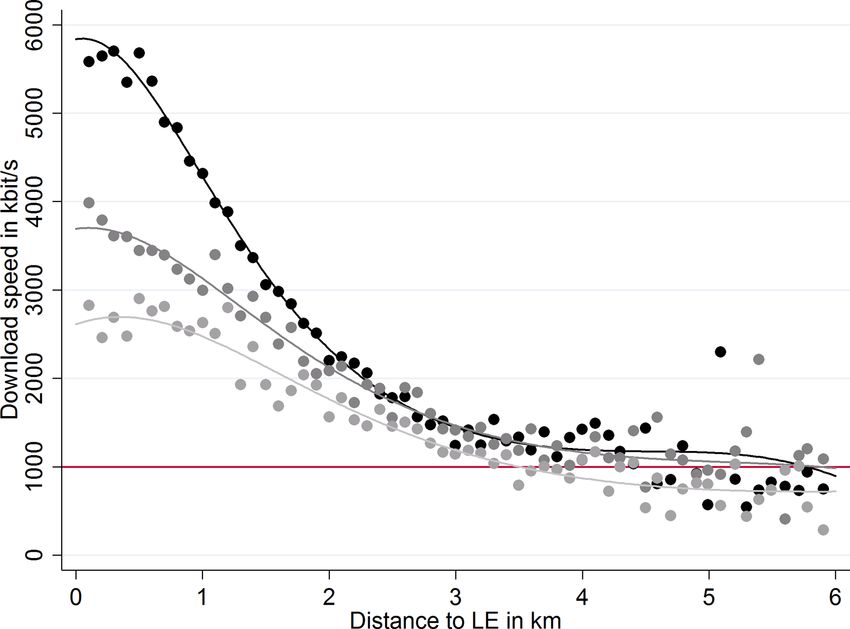
Ahlfeldt, Koutroumpis, and Valletti   Speed 2.0                                       589

benefits of the EU Digital Targets for different regions in England, which we compare
with available cost estimates. We find that increasing speed and connecting unserved
households pass a cost–benefit test in urban areas, whereas the case for universal
delivery in rural areas is not very strong.
     In order to provide reliable estimates of the valuation for broadband speed, we
need to avoid the circular problem that is present in all spatial concentrations of
economic activities. First, we need to separate the effect of high broadband speed on
property prices from other favorable locational characteristics, such as good transport

                                                                                             Downloaded from https://academic.oup.com/jeea/article/15/3/586/2847200 by guest on 29 September 2020
access or schools. Second, the available speed is endogenous to factors that determine
broadband demand and are likely correlated with property prices, such as high levels of
income and education levels. Thus, to avoid spurious correlation, we have to account
for macroeconomic shocks such as gentrification that potentially affect speed and
property prices simultaneously.
     We are able to trace the presence of broadband, and its speed, at the level of each
local delivery point, called a Local Exchange (LE) in the United Kingdom (this would
be called the Central Office in the United States). Every home can be supplied by
one and only one LE, which we can perfectly identify. Within a given LE area, the
distance between the user’s premises and the LE is, by far, the most important factor
affecting the performance of a given connection. In addition, LEs have been upgraded at
different points in time, with some exchanges boasting faster technologies than others.
The local distribution from legacy phone networks does not influence phone quality
but does affect broadband quality. This provides us with an ideal variation of speed
over time within an extremely small area. We are able to identify the causal effect
of digital speed on property prices from two alternative sources of variation. First,
we exploit a discontinuity across LE boundaries over time. Adjacent properties can
belong to the catchment areas of different LEs and, therefore, with different distances
to the exchange and possibly also different vintages of technology. Holding constant
all shocks to a spatially narrow area along the boundary of two LEs, the discontinuous
changes in speed that arise from LE upgrades at both sides of such a boundary provide
variation that is as good as random. In other words, we compare the house prices of two
properties, located next to each other, that are observationally equivalent in terms of
characteristics but for the speed available to each one of them. Second, we use variation
over time within LEs. Because we can hold constant any macroeconomic shock that
mutually determines property prices and upgrade decisions, which are made at the LE
level, the conditional variation in speed is plausibly exogenous. Both identification
strategies result in very similar estimates.
     Our work is related to two streams in the literature. In general, our methods
are common to a large literature in urban and public economics that has explored
capitalization effects of local public goods or nonmarketed externalities more generally
(Chay and Greenstone 2005; Davis 2004; Greenstone and Gallagher 2008; Linden and
Rockoff 2008). We use similar methods and show how they also can be used in settings
where, a priori, we would not think of an externality. Here, we deal with a market that
is largely competitive and privately supplied, but there are still capitalization effects:
a good part of the consumer surplus associated with broadband consumption seems to
go to the property seller as a scarcity rent, and not to the broadband suppliers.
590                                               Journal of the European Economic Association

    A second stream in the literature to which we contribute is related to the evaluation
of broadband demand and of the benefits associated with Internet deployment. At
a macro level, Czernich et al. (2011), using a panel of OECD countries, estimate a
positive effect that Internet infrastructure has on economic growth. Kolko (2012) also
finds a positive relationship between broadband expansion and local growth with the
US data, whereas Forman et al. (2012) study whether the Internet affects regional
wage inequality. Greenstein and McDevitt (2011) provide benchmark estimates of
the economic value created by broadband Internet in the United States. Some studies

                                                                                                       Downloaded from https://academic.oup.com/jeea/article/15/3/586/2847200 by guest on 29 September 2020
assess the demand for residential broadband: Goolsbee and Klenow (2006) use survey
data on individuals’ earnings and time spent on the Internet, whereas Nevo, Turner,
and Williams (2016) employ high-frequency broadband usage data from one ISP. To
our knowledge, ours is the first study to estimate consumer surplus from Internet usage
using property prices for a large economy.
    The rest of the paper is organized as follows. In Section 2, we describe the
development of broadband Internet in England and discuss the theoretical linkage
between broadband speed and property prices. Section 3 presents the empirical strategy.
The main results are shown and discussed in Section 4. Section 5 uses the empirical
findings to quantify the benefits for the EU 2020 digital targets. Finally, Section 6
concludes.

2. The Broadband Market

In this section, we first describe the recent development of broadband Internet in
England and then give an overview of its variation over time and space. We then
describe our data sources. Finally, we provide a simple theoretical model that links
broadband availability, and its speed, to property prices.

2.1. The Broadband Market in England

The market for Internet services in England6 is characterized by the presence of a
network, originally deployed by British Telecom (BT) during the first part of the 20th
century to provide voice telephony services. BT was state-owned until its privatization
in 1984. This network consists of 3,897 Local Exchanges (LEs). Each LE is a node of
BT’s local distribution network (sometimes called the “local loop”) and is the physical
building used to house internal plant and equipment. From the LE, lines are then further
distributed locally, by means of copper cables, to each building in which customers live
or work, which tend to be within 2 km from the LE. LEs aggregate local traffic and then
connect up to the network’s higher levels (e.g., the backbone) to ensure world-wide
connectivity, typically by means of high-capacity (fiber) lines.

6. The broadband description applies to the whole of the United Kingdom. However, since our property
data cover only England, we always refer to England alone throughout the paper.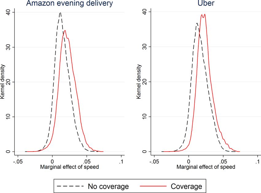
Ahlfeldt, Koutroumpis, and Valletti       Speed 2.0                                  591

    Although the basic topology of BT’s network was decided several decades ago,
technology has proven extremely flexible. The old copper technology, until the end
of the 1990s, provided a speed up to 64 kbit/s per channel via dial-up (modem)
connections. Without having to change the cables in the local loop, it has been
possible to supply high-speed Internet by installing special equipment in the LEs.
A breakthrough occurred with a family of technologies called digital subscriber
line (DSL), which use a wider range of frequencies over the copper line, thus
reaching higher speeds. The first major upgrade program involved bringing the ADSL

                                                                                            Downloaded from https://academic.oup.com/jeea/article/15/3/586/2847200 by guest on 29 September 2020
technology to each LE. BT began the program in early 2000 and took several years
to complete it. This upgrade could initially improve Internet speed by a factor of
40 compared to a standard dial-up modem and, afterwards, allowed speeds up to
8 Mbit/s.
    Along with technological progress, the regulatory framework and the competitive
landscape also evolved over the same period. Ofcom, the United Kingdom’s regulator
for communications, required BT to allow potential entrants to access its network
via the so-called “local loop unbundling” (LLU). LLU is the process whereby BT
makes its local network of LEs available to other companies. Entrants are then able
to place their own equipment in the LE and to offer services directly to customers.
LLU started to gain pace in 2005, and entrants have progressively targeted those
LEs located in more densely populated areas. Regulatory intervention is limited to
wholesale prices, whereas retail prices are freely set by competing providers. A further
major improvement occurred with ADSL2C. This upgrade, which allows for download
speeds, theoretically, up to 24 Mbit/s, started around 2007. It was first adopted by some
of the new LLU entrants, and BT followed with some lag. ADSL, LLU, and ADSL2C
are going to be major shifters of speed in our data, as they varied substantially over
time and by LE. In addition, all technologies based on DSL are “distance sensitive”
because their performance decreases significantly as you get further away from the
relevant LE.
    Of course, the diffusion of broadband Internet was not uniform across the United
Kingdom, and several demand and supply factors determined different penetration
rates across markets and over time. Nardotto et al. (2015) document how the entry
process took off around 2005, and show that entrants improved considerably the speed
available locally in each LE where they entered. First, local entry of new providers
was the main reason for the adoption of broadband Internet. In order to recover entry’s
large investment, entrants first unbundled the larger and more profitable LE markets,
and later expanded to cover a large share of the country. Second, the shape and the
size of the area covered by each LE was an important determinant of entrants’ costs.
Finally, rapid technological progress, along with entrants’ learning curves, decreased
costs over time.7
    Figure 1 shows the evolution of the share of English households in the catchment
area of LEs enabled with ADSL (black solid line) or with LLU entrants (gray solid

7.   See Chen and Savage (2010) for a related analysis for the United States.
592 Journal of the European Economic Association
Downloaded from https://academic.oup.com/jeea/article/15/3/586/2847200 by guest on 29 September 2020
F IGURE 1. Share of households with ADSL/LLU over time. Black (gray) lines refer to ADSL
(LLU) activation. Solid (dashed) lines refer to all households in England (NBS D Nationwide
Building Society transactions data set). [Color online]
line).8 We therefore cover the period that was crucial for the development of residential
Internet. The share of properties in our sample reflects very closely the technological
pattern in England (dashed lines), providing reassurance on its representativeness. In
Online Appendix A, we provide further empirical evidence, showing maps of how
these technological changes occurred by region and over time.
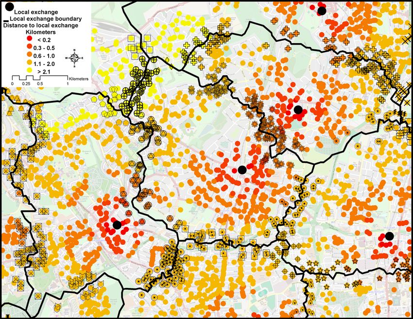
Figure 2 is a static map of a few LEs located north of London. The figure reports
the location of the relevant LEs in that area (big black dots), and their catchment areas,
based on the full postcodes served (black boundaries). Each grey dot represents the
location of one transaction in the property dataset, where lighter colors correspond
to increasing distances from the exchange (from red to yellow in the online version).
Black icons denote groups of properties that have been matched to common boundary
segments. These two figures show two important things that will inform our empirical
strategy. First, there is considerable variation both in the distance between premises
and the relevant LE (Figure 2), and in the technology available over time at a given LE,
which should have an impact on the available speed for a specific property (Figure 1).
We will, thus, be able to control for unobserved shocks to neighborhoods at very
disaggregated levels and restrict identification to variation that stems from changes
in the relative distribution of speeds within LEs over time. Second, there are enough
8. We do not show ADSL2C in order not to clutter the figure, but it would lie below the LLU curve.Ahlfeldt, Koutroumpis, and Valletti Speed 2.0 593
Downloaded from https://academic.oup.com/jeea/article/15/3/586/2847200 by guest on 29 September 2020
F IGURE 2. Distribution of properties and LE catchment areas. Black icons denote groups of
properties within 200 m of a shared boundary segment. The gray dots are transactions from the
NBS dataset. The black dots are the locations of LEs and the black boundaries are their catchment
areas, both from the Ofcom dataset. [Color online]
properties at the LE boundary allowing us to exploit discontinuities in speed increases
if one or both LEs are upgraded.
To complete the picture, broadband Internet can also be supplied via an alternative
cable network.9 The cable operator Virgin Media deployed its own network during
the 1990s, primarily for the purpose of selling cable TV. The topology of this network
is very different from that of BT. It covers roughly 50% of the premises in England,
concentrating its presence in urban areas and flat parts of the country. The cable
network can be upgraded to support broadband only if an area is already covered by
cable, which has not expanded its reach since the 1990s. Cable technology, since it
also aims at providing TV, is typically faster than ADSL, and broadband speed does
not degrade substantially with distance from the exchange.
9. At the beginning of 2010, BT had a retail market share of 28%, the cable operator had a market share of
approximately 22%, and the entrants (the main ones are TalkTalk, Sky, O2, and Orange) had the remaining
50% of the market. There has been little investment in fiber within the local loop, and during the period we
consider here, there has been limited take-up of high-speed connections based on 3G cellular technology.
Broadband access via Wi-Fi technologies, on the other hand, is included in our dataset.594 Journal of the European Economic Association
2.2. Raw Data
Our dataset stems from several sources. The main block concerns the development of
broadband in England over the period 1995–2010. Ofcom has made available to us all
the information it collects on the broadband market for regulatory purposes. The dataset
comprises quarterly information at the level of each of the 3,897 LEs in England. For
each local exchange, we know the precise coverage of BT’s local network—that is,
all the specific full postcodes served by a certain LE—and, therefore, we know how
Downloaded from https://academic.oup.com/jeea/article/15/3/586/2847200 by guest on 29 September 2020
many buildings and total lines can eventually have broadband. We remark that a full
postcode unit contains about 10–15 households, which are all connected to the same
LE.10
We can identify when a LE was upgraded to ADSL or ADSL2C, and if and when
it attracted entrants via LLU. We also know, in the catchment area of the LE, whether
or not cable is available. Finally, we know how broadband penetration varies over time
in a given LE, as we are told the total number of subscribers (via BT, via an entrant,
or via cable), which can be compared to the total lines available locally to compute
broadband penetration.
This detailed information was supplemented with information on broadband speed
tests carried out by individuals in 2009 and 2010. We obtained three million tests
from a private company.11 For each individual/speed test, we observe the operator, the
contract option chosen by the user, the location (full postcode), as well as when the
test was carried out. Thus, we can calculate the distance between the user’s premises
and the exact location of the relevant LE. The dataset contemplates two measures of
performance: download speed and upload speed. We focus on the former, which is,
by far, the more important feature for residential household users. It is important to
note that, throughout the whole paper, we refer to the speed measured in the dataset
on speed tests as “actual” speed. This is not the same as the speed typically advertised
by operators in their plans, to which we refer as “nominal” speed.12
For the analysis of the capitalization effects of broadband capacity, we use
transactions data related to mortgages granted by the Nationwide Building Society
between 1995 and 2010. The data for England comprise more than one million
observations,13 and include the price paid for individual housing units along with
detailed property characteristics. These characteristics include floor space (m2 ), the
10. A full (typically, seven digit) postcode in the United Kingdom captures a narrowly defined area.
There are approximately two million postcodes in the United Kingdom. A full postcode is not an address,
but still covers areas that are on average within a radius of 50 m, which gets even narrower in densely
populated areas (e.g., 20 m in London).
11. http://www.broadbandspeedchecker.co.uk, accessed December 2015. More information is provided
in Section 3.1.
12. The discrepancy for the top plans is large and amounts to a factor of 4 (results are available on
request from the authors). This factor is also in line with independent findings of Ofcom; see, for example,
http://stakeholders.ofcom.org.uk/market-data-research/other/telecoms-research/broadband-speeds/
speeds-nov-dec-2010/, accessed December 2015, and Figure 1.2 in particular.
13. This represents 10% of all mortgages issued in England over the period.Ahlfeldt, Koutroumpis, and Valletti Speed 2.0 595
type of property (detached, semi-detached, flat, bungalow, or terraced), the date of
construction, the number of bedrooms and bathrooms, garage or parking facilities,
and the type of heating. There is also some buyer information, including the type of
mortgage (freehold or leasehold) and whether they are first-time buyers. Note that the
transaction data include the full UK postcode of the property sold, allowing it to be
assigned to grid-reference coordinates.
With this information, it is possible with Geographic Information System (GIS)
software to calculate distances to LEs. Furthermore, it is possible to calculate distances
Downloaded from https://academic.oup.com/jeea/article/15/3/586/2847200 by guest on 29 September 2020
and other spatial measures (e.g., densities) for the amenities and environmental
characteristics such as National Parks, as well as natural features such as lakes,
rivers, and coastline. The postcode reference also allows a merger of transactions
and various household characteristics (median income and ethnic composition) from
the UK census; natural land cover and land use; and various amenities, such as access to
employment opportunities, retail services, cultural and entertainment establishments,
school quality, and measures of online services (e.g., Amazon evening delivery, Uber
fleet services). A more-detailed description of all the data used is in Online Appendix
B. In Online Appendix C.1, we also show that the distributions of other observable
amenities do not differ discontinuously on the two sides of a LE.
2.3. A Simple Conceptual Model
Unlike local public goods such as good (public) schools, public safety, or air quality,
which are often analyzed in the house price capitalization literature, households
subscribed to broadband pay a price to their Internet provider. A capitalization
effect of broadband is, therefore, not an obvious feature of the spatial equilibrium.
The purpose of this section is to introduce a simple model that links broadband
speed to property prices. Our intention is not to introduce a model for structural
estimation, but, rather, to think about this link in a simple and transparent
manner.
For this purpose, imagine that there are n areas, indexed by j D 1, . . . , n. In each
area there is a population of household buyers whose total number is normalized to
unity. The value of a property is denoted as V, which can be made dependent on all
its characteristics, such as number of rooms, local amenities, and so forth, except for
broadband availability, which is described next. The price of a property is denoted
as P.
Households are heterogeneous in their value of using broadband. Value can derive
from different sources—from leisure (surfing the Internet) to being able to work from
home. We are not interested in the particular channel, but simply imagine that people
are heterogeneous in the way that they use and value the Internet. Let vlog(qj ) denote
the gross utility of household type v using a broadband of quality qj , where qj is the
Internet quality available in area j, for instance, the speed of the connection. This
specification reflects diminishing marginal returns to speed, as well as the fact that
everybody would enjoy faster connections, ceteris paribus, despite heterogeneity in596 Journal of the European Economic Association
tastes. The distribution of household types v is assumed to be uniform between 0 and
aj in area j, thus the density is 1/aj .14
The consumers’ choice is whether or not to purchase broadband, conditional on
having bought a property. We normalize the payoffs from not using broadband to zero.
Broadband of quality qj is sold at a price pj . Since broadband is a durable good, all these
variables are to be interpreted as flows in each period. We also assume that, at some
period in the future denoted as Tj , some alternative technology that does not need fixed
lines becomes available, and it will be preferred by all customers (because it is cheaper
Downloaded from https://academic.oup.com/jeea/article/15/3/586/2847200 by guest on 29 September 2020
or better, or both). Think, for instance, of Long-Term Evolution (LTE) mobile technol-
ogy replacing fixed broadband. The key point is that this technology will not be bundled
with the property anymore, but it will represent a completely separate purchase that has
nothing to do with a property. The cumulative utility for type v from fixed broadband
RT
access is thus [vlog(qj ) pj ]j , where j D 0 j e t dt D .1 e Tj /= and is
the discount rate. Note that, if the alternative technology never becomes available,
Tj ! 1 and the discount factor j simplifies to 1/, that is, the value of a perpetuity.
Households whose value of broadband is high enough will purchase a broadband
connection. In particular, the marginal broadband household in area j is defined by
vj D pj /log(qj ), and all types between vj and aj purchase broadband in that area in
every period.
On the property supply side, we assume that homes in a given area are scarce, such
that sellers can always extract all buyers’ net surplus. Alternatively, we can also assume
that sellers are able to observe buyers’ types—during negotiations, for example—and
make take-it-or-leave-it offers leading to the same outcome. Households are assumed
to be perfectly mobile, with reservation utility U. In a spatial equilibrium, house prices
in area j will, therefore, be
(
V U for v < vj .households without broadband/;
Pj D
V U C Œv log.qj / pj j for v vj .households with broadband/:
(1)
Since the econometrician will not observe types, but just the average prices in a
given area with or without broadband subscription, we can calculate these averages
from (1) as
Z
.V U /vj aj ŒV U C .vlog.qj / pj /j
Pj D C dv D V U C Kj j ;
aj vj aj
(2)
where
.aj qj pj /Œ.aj qj C pj /log.qj / 2qj pj
Kj :
2aj qj2
14. The example is generalizable to a more general distribution function F(v) that satisfies the monotone
hazard rate condition.Ahlfeldt, Koutroumpis, and Valletti Speed 2.0 597
It is a matter of simple maths to show that15
2
∂P j ∂K ∂P j
(a) ∂qj D j ∂q j > 0 and ∂qj2
< 0,
j
∂P j ∂Kj
(b) ∂aj D j ∂aj > 0,
∂P j ∂j
(c) ∂Tj D Kj ∂Tj > 0.
Downloaded from https://academic.oup.com/jeea/article/15/3/586/2847200 by guest on 29 September 2020
Equation (2) and the associated comparative statics confirm the intuition that
broadband speed gets capitalized into house prices. In particular (part (a)), prices
should increase in those areas with higher available speed qj , and they increase at a
decreasing rate (decreasing returns to speed). Prices should also increase (part (b)) in
those areas where there is a higher willingness-to-pay (WTP) for the Internet, because
of the heterogeneity in the population that we have modeled via aj (which may be
related to income, something we do observe at the level of an area in our data). Places
with the highest price premium for speed are likely also to have residents with the
greatest taste for speed. Equation (2) also makes a point about sorting: the coefficient
estimates from the hedonic price regressions that we will run should return the mean
marginal valuations of properties (Bayer, Ferreira, and McMillan 2007), and we need
to be careful when conducting policy evaluation involving levels of speed different
from those observed. Finally (part (c)), the capitalization effect depends on whether
there is an expectation that fixed line broadband will be displaced by technologies
that are not bundled with the property. If these technologies do not exist, our results
effectively capture a perpetuity in the value of broadband, else they will capture only
the net present value from a shorter period.
The model also has an ancillary prediction about broadband penetration in a given
area. This provides a useful check for the robustness of our main results and a way to
evaluate the channels through which the capitalization effect operates. Penetration is
given by
vj pj
Penetration D 1 D1 ; (3)
aj aj log.qj /
which is also increasing in speed qj , and at a decreasing rate. Equation (3) also says
that—ceteris paribus—penetration in a certain area is driven by Internet characteristics
(qj and pj ) and by population characteristics (aj ), but not amenities that depend
themselves on the availability of fast broadband (e.g., cybercafés).
Note that we left the broadband subscription price pj unmodeled, thus the main
prediction that property prices increase with speed is independent of the precise market
structure of the local broadband market: intuitively, it is stronger when the broadband
15. One just needs that pj < aj log (qj ), which must hold true for the problem to make economic sense,
otherwise, not even the household with the highest willingness to pay would get a broadband subscription.598 Journal of the European Economic Association
supply is very competitive, but it holds even for a monopolist provider. In other words,
there are limits to the consumer surplus that ISPs can appropriate when speed increases.
Competition is the upper limit, in fact, broadband subscription fees cannot increase
with willingness to pay for speed when competition is intense, as they will just reflect
costs. But even a monopolist would be constrained by its inability to observe different
types perfectly and would, therefore, leave some information rent to higher types.
Our approach presumes that all remaining consumer surplus from broadband, over
and above the broadband price paid to the provider, is appropriated by the seller of
Downloaded from https://academic.oup.com/jeea/article/15/3/586/2847200 by guest on 29 September 2020
the property. If this were not the case, then the impact that broadband might have on
property prices would underestimate the consumer surplus from broadband use. We
will return to this point in our conclusions.
3. Empirical Framework
The primary aim of our empirical strategy is to provide a causal estimate of the impact
of high-speed broadband supply on house prices. The empirical challenge in estimating
this causal effect is to separate the effect of broadband supply from other unobserved
and potentially correlated determinants of house prices. In particular, we must ensure
that there are no omitted variables that simultaneously determine broadband supply and
house prices. We argue that robust identification can be achieved from discontinuous
variation in speed over time and across LE boundaries. Variation over time helps
disentangle the effect of broadband supply from unobserved (spatially) correlated
locational factors, such as good transport access or better schools. By further placing
properties into groups that are near to and share the same LE boundary, it is possible
to control for shocks at a very small spatial level. We argue that variation in speed over
time across a LE boundary within such a small area is plausibly exogenous and as good
as random. We also run an alternative identification that relies on the comparison of
house prices to broadband supply over time and within LE areas. Decisions that affect
the broadband supply of a property are generally taken at the level of the LE serving
an area. Conditional on shocks to a certain LE catchment area—such as a sudden
increase in income or education of the local population—within-LE variation in speed
over time that results from the distance of a property from the relevant exchange can
be assumed to be exogenous.16
We follow the popular hedonic pricing method to separate various determinants
of property prices. Rosen (1974) has provided the microfoundations for interpreting
parameters estimated in a multivariate regression of the price of the composite housing
good against several internal and locational characteristics as hedonic implicit attribute
prices. Underlying the hedonic framework is the idea that, given free mobility in spatial
16. Note that local exchange areas are relatively small. The median radius of a local exchange area is
less than 6 km, as far as old voice telephony services are concerned. As for broadband, the area where it
can be supplied effectively is smaller, up to 2–3 km from the local exchange, as shown below in the results.
In cities, the median radius of a LE is further reduced—for example, less than 2 km in London.Ahlfeldt, Koutroumpis, and Valletti Speed 2.0 599
equilibrium, all locational (dis)advantages must be offset by means of property price
capitalization. There is a long tradition in the literature—dating back at least as far
as Oates (1969)—that made use of the hedonic method to value local public goods
while holding confounding factors constant. One of the typical challenges faced by
such hedonic valuation studies is the potential for bias due to omitted variables that are
correlated with a phenomenon of interest. Recent applications of the hedonic method
have tackled this problem by making use of variation over time to identify the effects of
locational improvements from unobserved time-invariant locational factors (Ahlfeldt
Downloaded from https://academic.oup.com/jeea/article/15/3/586/2847200 by guest on 29 September 2020
and Kavetsos 2014; Chay and Greenstone 2005; Davis 2004; Linden and Rockoff
2008).
Both of the empirical specifications we employ are drawn from this line of research.
We model the (log) price of a property sold at a full postcode i at time t, served by
LE j and lying on the LE boundary segment k as a function of the available broadband
speed, as well as a range of internal and locational property characteristics that are
partially observed and partially unobserved. Our baseline empirical specification is a
variant of a spatial boundary discontinuity design (BDD):
X2 X4
log.Pijkt / D ˛m .Sijt /m C .DISTij / n
C Xi0 t
mD1 nD1 n
C kt C 'j C "ijt ; (4)
where Sijt is the available broadband speed, and DISTij is the Euclidian distance from
a postcode i to the relevant LE j. We use a quadratic specification for broadband
speed to allow the property price to vary non-linearly with speed, as predicted by
our simple model. The distance polynomial controls for unobserved time-invariant
locational characteristics that are correlated with distance to the LE. As discussed in
more detail in the next section, our variable of interest Sijt is constructed using fourth-
order polynomials of DISTij following an engineering literature. Because Sijt varies over
time, the speed effect, after controlling for the time-invariant distance trend, is identified
from variation over time. The control variable approach is therefore equivalent to
postcode fixed effects in terms of its power to absorb unobserved locational effects
that are correlated with Sijt . Compared to the alternative of using postcode fixed
effects, we prefer this control variable approach because of a relatively limited number
of repeated sales at the same postcode level.17 Xi0 is a vector of property and locational
characteristics discussed in the data section. This is interacted with a full set of year
effects, so that t is a matrix of implicit prices for attribute-year combinations. ' j
is a dummy to control for unobserved time-invariant LE effects. Finally, k indexes
properties that lie along the same boundary segment that separates two LE areas. We
match properties in LE j to the nearest property in LE l 6D j and define a common
time-varying fixed effect k t for properties in j whose nearest neighbor is in l and vice
17. Less than half (15%) of the full postcodes in the Nationwide data set contain two (three) or more
transactions. On average, there are 2.15 transactions per full postcode over the 15-year period we cover.600 Journal of the European Economic Association
versa. These fixed effects ensure that we identify from a differential increase in speed
at the two sides of the boundaries, holding constant all other time-varying effects that
are common to both sides of a boundary. Figure 2 illustrates the matching of properties
across adjacent LEs.
This specification exploits the discontinuity at the boundaries between LEs.
Overall, there are 86,569 LE boundary year effects in our data, which denote
boundary segments that are common to the same two LEs. With this specification,
we attribute differences in price changes over time across a common boundary to the
Downloaded from https://academic.oup.com/jeea/article/15/3/586/2847200 by guest on 29 September 2020
respective differences in speed changes over time. We restrict our sample to properties
that are close to a LE boundary to explicitly exploit the spatial discontinuities in speed
changes that arise across a LE boundary if the broadband infrastructure is altered. We
note that a discontinuity arises not only if just one of two adjacent LEs is upgraded,
but also if both LEs are upgraded, and the distance to the respective LEs differs
significantly at both sides of the LE boundary. Because, at a local level, the allocation
of a property to either side of the same boundary is as good as random, it is unlikely
that unobserved shocks affect speed and property prices on one side of the boundary
but not on the other. Even in this unlikely event, such shocks are absorbed by the LE
boundary year effects.
We also estimate an alternative specification in which we replace the LE boundary
year effects with a set of 37,804 LE year fixed effects ' jt that control for all
macroeconomic shocks at the LE level:
X2 X4
log.Pijt / D ˛m .Sijt /m C .DISTij / n
C Xi0 t C 'jt C "ijt : (5)
mD1 nD1 n
With this specification we focus on a different source of variation, compared to
equation (4). Instead of exploiting discontinuous variation in speed over time across
LE boundaries we now identify exclusively from continuous variation in speed over
time within LEs. In estimating equation (5) we also use the universe of transactions
and variation in speed, which helps addressing the external validity problem inherent
to all boundary discontinuity designs. This specification delivers a causal effect of
broadband speed on house prices under the identifying assumption that year-specific
shocks that potentially determine broadband capacity are uncorrelated with distance
to the LE within the area that the LE serves. This is a plausible assumption for
two reasons. First, any change to the LE technology will affect the entire catchment
area served by the LE, so it is rational for broadband suppliers to base decisions on
the average trend in this area. It is, therefore, unlikely that within-LE shocks that
might affect property prices—for example, an income increase among the population
near the LE relative to other areas—would also affect the technological upgrading
decisions above and beyond their effect on the LE area average, which is captured by
' jt . Second, LEs serve relatively small areas, with a layout that was defined decades
ago and boundaries that do not line up with spatial statistical units, such as census
wards. The catchment area of each LE is typically known only to providers and is
not used to create any other related boundaries. Reliable information on year-on-year
changes at the sub-LE area level is difficult to obtain, which makes it unlikely thatAhlfeldt, Koutroumpis, and Valletti Speed 2.0 601
providers would be able to respond within LE-area shocks even if they wanted to.18
This specification is arguably more open to criticism because there may be within-LE
trends in property prices that are correlated with distance to the LE, something that
is absent with the previous specification relying on the boundary discontinuity. It is
noteworthy that the interactions of year effects and attributes Xi0 flexibly control for
property price trends that are correlated with any of the observable structural and
locational characteristics. Conditional on these controls, it is less likely that within-LE
trends, which are correlated with but not causally related to changes in speed within
Downloaded from https://academic.oup.com/jeea/article/15/3/586/2847200 by guest on 29 September 2020
LEs over time, confound the estimated broadband speed effect. Moreover, we can also
use difference-in-differences techniques to reassure ourselves that, conditional on the
strong controls employed, there are no within LE trends correlated with distance to the
LE that could lead to spurious broadband supply effects.
We finally note that equations (4) and (5) are complementary. Adding LE year
fixed effects ' jt to equation (4) would partially absorb the identifying discontinuous
variation in speed over time across LE boundaries. Likewise, adding LE year
boundary fixed effects k t to equation (5) would partially absorb the identifying
continuous variation in speed over time within LEs. Because the two equations are
designed to identify the broadband capitalization effect from two different types of
variation, consistent estimates will be particularly indicative of their robustness.
3.1. The Relationship Among Technology, Distance, and Speed
As said above, we have very detailed information on the exact broadband capacity to
deliver achievable speeds at a specific property at a high spatial detail, but not over
the entire period. We know, however, the technology available in each LE at different
points in time. We now establish the technological relationship between actual Internet
speed, the technology of a LE, and the distance from a test location to the LE, using the
comprehensive data set of Internet speed tests in the sub-period 2009–2010. Combining
both ingredients, it is possible to generate the micro-level Internet speed panel variable
we require for a robust identification of the causal effect of broadband capacity on
house prices.
We model broadband actual speed as a function of LE characteristics and the
distance to the LE, as well as the interaction between the two. In doing so, we first
need to account for a significant proportion of speed tests that are likely constrained
not only by technological limitations (distance to the LE and LE characteristics), but
also by the plans users have chosen to subscribe to. In other words, speed can be low
not because technology is limited, but because a subscriber with small consumption
choses a plan with limitations. We want to get rid of these plans so that we can unravel
the true speed that a certain technology can potentially supply. To identify the plans
18. It is telling that all the regulatory analysis done by Ofcom, which relies on information supplied by
the broadband operators, is, indeed, conducted at the LE level, instead of at a more disaggregated level,
such as street cabinets. This is because the regulator believes that the relevant market for business decisions
is the LE, which is where most investments have to be sunk.602 Journal of the European Economic Association
that do not constrain broadband speed beyond the technological limitations of the LE,
we run the following auxiliary regression:
X12 X23 X6
log.Sijt / D ˛m C ˛h C ˛w
mD2 hD1 wD1
X62 X60
C ˛p C ˛d C 'jt C "ijt ; (6)
pD1 d D2
where Sijt is the actual broadband speed test score measured at postcode i served by
Downloaded from https://academic.oup.com/jeea/article/15/3/586/2847200 by guest on 29 September 2020
local exchange j at time t. ˛ m are month of the year effects (baseline category is
January), ˛ h are hour of the day effects (baseline category 0 h), ˛ w are day of the week
effects (baseline category Sunday), ˛ p are Internet plan effects (baseline category is
missing information), ˛ d are distance to LE effects captured by 100 m bins (e.g., 2
covers distances from 150 to 250 m, baseline category is 0–150 m), and ' jt are a
set of LE-year specific fixed effects that capture unobserved LE characteristics in a
given year. For the ensuing analysis, we keep observations whose ˛ p falls in the upper
quartile, as the plans that realize the fastest actual speeds are unlikely to be constrained
by the provider.
Using this subsample of speed tests that should be constrained only by technology,
we then establish the technological relationship between available actual broadband
speed Sijt and distance to the relevant LE (DISTij ) for each technological category
Q D fADSL, ADSL C LLU, ADSL2Cg in separate regressions of the following
type:
X12 X23 X6
log.Sijt / D ˛mQ C ˛hQ C ˛wQ
mD2 hD1 wD1
X4
C ˛nQ .DISTij /n C 'jQ C !tQ C "ijtQ : (7)
nD0
The fourth-order polynomial is used to capture the non-linearities reported in the
technical literature.19 Since we drop 75% of the observations compared to equation (6)
and split the remaining sample into three categories in order to find technology-specific
effects, we account for location and year effects separately, rather than accounting for
their interaction, to save degrees of freedom in sparsely populated LEs. Based on the
Q
estimated distance decay parameters ˛ nQ and the known Q-type upgrade dates Tj , it
is then straightforward to predict the available actual broadband speed at any postcode
i that is served by a LE j over the entire period:
(
ISDN D 128 kbit=s if t < TjADSL
Sijt D hP i : (8)
4 Q Q0
nD0 ˛nQ .DISTij / if Tj t < Tj
n
exp
19. For a list of the factors that affect local broadband speed, see, for example, the explanation provided by
BT: http://bt.custhelp.com/app/answers/detail/a id/7573/c/, accessed December 2015. A detailed analysis
of the factors that affect the performance of ADSL networks is found in Summers (1999). We note that the
choice of a fourth-order polynomial for distance was dictated by its goodness of fit. There was no gain in
going toward higher orders.Ahlfeldt, Koutroumpis, and Valletti Speed 2.0 603
TABLE 1. Speed results.
(1) (2) (3) (4)
log of download speed (kbit/s)
Broadband Broadband Broadband
Technology ADSL ADSLCLLU ADSL2C Cable
Distance from test 0.184 0.057 0.053 0.016
Downloaded from https://academic.oup.com/jeea/article/15/3/586/2847200 by guest on 29 September 2020
postcode to LE in km (0.145) (0.121) (0.071) (0.032)
Distanceˆ2 0.293 0.287 0.491 0.016
(0.097) (0.097) (0.055) (0.029)
Distanceˆ3 0.058 0.070 0.141 0.001
(0.024) (0.028) (0.017) (0.010)
Distanceˆ4 0.003 0.005 0.011 0.001
(0.002) (0.002) (0.002) (0.001)
Constant 7.869 8.214 8.672 8.334
(0.098) (0.065) (0.036) (0.017)
LE effects Yes Yes Yes Yes
Month effects Yes Yes Yes Yes
Day of the week effects Yes Yes Yes Yes
Hour of the day effects Yes Yes Yes Yes
Year effects Yes Yes Yes Yes
r2 0.358 0.318 0.242 0.034
N 53,961 64,447 310,256 290,067
Notes: Only observations falling into the top-quartile of contracts are used in the regressions. Standard errors in
parentheses are clustered on LEs. p < 0.1, p < 0.05, p < 0.01.
This compact formulation says that, before broadband is rolled out in LE j, the line
is served with a basic ISDN technology, as a voice telephony line is in place. Then,
ADSL brings its upgraded speed at any period after TjADSL . The decay parameters
0
may further change if the LE additionally receives, at a certain point in time TjQ ;
technology Q0 D fADSL C LLU, ADSL2Cg.
We start by reporting the results on the physical relationship among speed,
technological characteristics of the LE, and distance between the premise and the
LE, as described by model (7). Our findings are shown in Table 1.
Although, due to space limitations, we do not detail the various fixed effects in the
table, they all show a very reasonable behavior. The time of day is an important factor:
the average connection speed reaches its peak at 5 a.m., when download speed is about
12% faster than the reference speed at midnight. It then gradually declines, with speed
3% lower at noon, 11% lower at 6 p.m., and close to 20% lower at 8 p.m., when the
worst daily speed is attained. From then on, the average speed of a connection gradually
increases until 5 a.m. The day of the week also determines average speed: it is lowest
over the weekend, when residential users tend to be at home. These findings are due
to obvious local congestion when most people are online simultaneously. Congestion604 Journal of the European Economic Association
Downloaded from https://academic.oup.com/jeea/article/15/3/586/2847200 by guest on 29 September 2020
F IGURE 3. Distance decay by LE type. Black lines and dots indicate ADSL2C LEs, dark
(respectively, light) gray lines and dots are ADSL LEs with (respectively, without) LLU. [Color
online]
is, thus, another facet of speed that shows striking analogies in the digital and the real
worlds (see, e.g., Couture et al. 2012; Duranton and Turner 2011).
Turning to the impact of distance, which is of more direct interest for our purposes,
this is shown in columns (1), (2), and (3) of Table 1 for ADSL, LLU, and ADSL 2C,
respectively. Distance plays a statistically very significant role for all of them. Table 1,
column (4) also runs a placebo test. The cable technology, which is available only in
some parts of the country, does not rely on copper wires and does not suffer from
distance-decay problems. Thus, the distance of a home from any exchange should not
impact speed. Column (4) reports the results for one set of cable contracts offered by
the cable provider, and, indeed, distance is found to have no impact.
One way of showing the relevance of the results is to evaluate the fit of the
polynomial approximation. We estimate the distance relationships replacing the
polynomial, as estimated in Table 1, with a set of 100 m distance bin effects, as
used in equation (6). Results are shown in Figure 3. Solid lines are the fourth-order
polynomials (from Table 1) fitted into the raw data (not the dots). The dots indicate
the point estimates of 100 m bins obtained in separate regressions for each technology.
The fit is quite striking, especially for distances up to 5 km from the LE—for greater
distances, there is also more noise because there are few observations beyond that
distance. We are, thus, confident that we can approximate the real speed sufficiently
precisely so that attenuation bias can be ignored in equations (4) and (5). We further
note that we use estimated parameters of a physical relationship that depends on
distance and LE technology to approximate our speed capacity variable.You can also read