D4.5 Activity Monitoring and Lifelogging v2 - Dementia Ambient Care: Multi-Sensing Monitoring for Intelligent Remote Management and Decision ...

D4.5
Activity Monitoring and Lifelogging v2

Dementia Ambient Care: Multi-Sensing Monitoring
 for Intelligent Remote Management and Decision
 Support

 Dem@Care - FP7-288199

FP7-288199
D4.5 – Activity Monitoring and Lifelogging v2

Deliverable Information
Project Ref. No. FP7-288199
Project Acronym Dem@Care
 Dementia Ambient Care: Multi-Sensing Monitoring for Intelligence
Project Full Title
 Remote Management and Decision Support
Dissemination level: Public
Contractual date of delivery: Month 40, February 2015
Actual date of delivery: Month 41, March 2015
Deliverable No. D4.5
Deliverable Title Activity Monitoring and Lifelogging v2
Type: Report
Approval Status: Approved
Version: 1.4
Number of pages: 70
WP: WP4 Situational Analysis of Daily Activities
 T4.1 Visual Perception, T4.2 Audio Sensing. T4.3. Instrumental
Task:
 Activities Monitoring, T4.4. Lifelogging
WP/Task responsible: WP4/UB1
Other contributors: INRIA, CERTH, DCU

 Duc Phu Chau (INRIA),
 Vincent Buso (UBX),
Authors (Partner)
 Konstantinos Avgerinakis, Alexia Briassouli (CERTH),
 Feiyan Hu, Eamonn Newman (DCU),

Responsible Eamonn Newman
 Name
Author
 Email eamonn.newman@dcu.ie
 Ceyhun Baruk Akgul (Vispera)
Internal Reviewer(s)

EC Project Officer Stefanos Gouvras
 Deliverable D4.5 includes the description of the final versions of
 Dem@Care tools for visual data analysis and their evaluation on the
 datasets obtained within Dem@Care for posture recognition, action
 recognition, activity monitoring and life-logging. D4.5 extends
Abstract deliverable D4.2, which provided a study of the state of the art and a
(for dissemination) description of the first set of tools, by improving on the methods and
 expanding the experimental evaluation. The integration status of all
 visual processing components produced in this work package and
 their respective usage in pilots is also presented here, reflecting their
 impact of research outcomes in real-world Dem@Care applications.

 Page 2

FP7-288199
D4.5 – Activity Monitoring and Lifelogging v2

Version Log
 Version Date Change Author
 0.1 03/02/2015 Template for circulation Eamonn Newman (DCU)
 0.2 24/03/2015 Multi-camera tracking Duc Phu Chau
 0.3 – 0.7 27/03/2015 Initial complete template All
 0.8 28/03/2015 Technical Chapters for review Eamonn Newman (DCU)
 0.9 31/03/2015 Added Preamble, Intro, Concl. Eamonn Newman (DCU)
 1.0 15/11/2015 Added Human Activity Recognition section Kostas Avgerinakis (CERTH)
 1.1 23/11/2015 Addition of Integration and Pilot Usage Thanos Stavropoulos (CERTH)
 Section
 1.2 25/11/2015 Revision of entire D4.5 Alexia Briassouli (CERTH)
 1.3 30/11/2015 Additional revisions to D4.5 Alexia Briassouli (CERTH)
 1.4 1/12/2015 Final revisions to D4.5 Alexia Briassouli (CERTH)

 Page 3

FP7-288199
D4.5 – Activity Monitoring and Lifelogging v2

Executive Summary
D4.5 presents the final version of the audio-visual analysis tools developed for Dem@Care
and deployed in the integrated system and project pilots. The aim of the audio-visual analysis
has been the assessment of the individual’s overall status through the recognition of activities
of daily living for monitoring of behavioural and lifestyle patterns, cognitive status, mood.
Their integration into the final system enhances the description of the person’s status and the
progression of their condition due to the complementarity of the sensor data and the higher
level information extraction through Semantic Interpretation (SI). The results are expected to
provide new insights into dementia and its evolution over time, as well as the early detection
of deterioration in the individual’s status. An initial version of the tools developed within
Dem@Care and the first methods used was described in D4.2, while D4.5 presents their final
versions that expand and improve upon the previous ones. Finally, D4.5 presents real world
experimental evaluations of tools in the integrated Dem@Care system deployed in the pilots.

This report consists of 4 main chapters, following the structure of D4.2.
Chapter 2 describes the research conducted for tracking individuals through a scene using
multiple cameras, and shows how the proposed approach improves on the state of the art
algorithms for single camera tracking.
Chapter 3 presents the research carried out on video analysis for Action Recognition through
Object Recognition and Room Recognition on video data from a wearable camera.
Chapter 4 describes the work done for Activity Recognition and Person Detection from video
and RGB-D cameras.
Chapter 5 presents Periodicity Detection on longitudinal lifelog data where signal analysis
techniques are used to identify routines and periodic behaviour of an individual.
Chapter 6 presents a holistic component integration and pilot usage section, which
summarizes this entire Work Package contributions of research and development, to real-
world piloting and the clinical results in the context of Dem@Care.

 Page 4

FP7-288199
D4.5 – Activity Monitoring and Lifelogging v2

Abbreviations and Acronyms

 ADL Activities of Daily Living
 BB Bounding Box
 BoVW Bag of Visual Words
 CSV Comma Separated Values
 DTW Dynamic Time Wrapping
 EDM Euclidean Distance Mean
 FPS Frames Per Second
 GMM Gaussian Mixture Model
 GPS Global Positioning System
 HOF Histogram of Optical Flow
 HOG Histogram of Oriented Gradients
 IADL Instrumental Activities of Daily Living
 MCI Mild Cognitive Impairment
 PMVFAST Predictive Motion Vector Field Adaptive Search Technique
 PnP Perspective - n - Point
 PSD Power Spectral Density
 PwD Person with Dementia
 RANSAC Random Sample Consensus
 RGB-D Red Green Blue - Depth
 SURF Speeded Up Robust Features
 SVM Support Vector Machine

 Page 5

FP7-288199
D4.5 – Activity Monitoring and Lifelogging v2

 Table of Contents

 INTRODUCTION........................................................................................ 11

 PEOPLE TRACKING FOR OVERLAPPED MULTI-CAMERAS .................... 12
2.1 Introduction ............................................................................................................ 12
2.2 Proposed Multi-camera Tracking Approach ......................................................... 12
 2.2.1 Description of the Proposed Approach.............................................................................. 12
 2.2.2 Mono-camera tracking ..................................................................................................... 12
 2.2.3 Trajectory Association ..................................................................................................... 12
 2.2.4 Trajectory Merging .......................................................................................................... 14
2.3 Discussion and results ............................................................................................. 15
2.4 Conclusion ............................................................................................................... 17
2.5 References ............................................................................................................... 17

 ACTION RECOGNITION ............................................................................ 19
3.1 3D Localization From Wearable Camera .............................................................. 19
 3.1.1 Reconstruction of an apartment from a wearable camera................................................... 19
 3.1.2 Keyframe Selection .......................................................................................................... 20
 3.1.3 Sub-map Reconstruction .................................................................................................. 20
 3.1.4 Relative Similarity Averaging .......................................................................................... 21
 3.1.5 Qualitative Results ........................................................................................................... 21
 3.1.6 Metric Localization from a wearable camera .................................................................... 22
 3.1.7 Conclusion and Future Work ............................................................................................ 25
3.2 Object recognition ................................................................................................... 26
 3.2.1 Objectives ........................................................................................................................ 26
 3.2.2 Goal-oriented top-down visual attention model ................................................................. 27
 3.2.3 Experiments and results .................................................................................................... 34
 3.2.4 Conclusions ..................................................................................................................... 39
3.3 References ............................................................................................................... 39

 ACTIVITY MONITORING .......................................................................... 42
4.1 Introduction ............................................................................................................ 42
 4.1.1 Objectives ........................................................................................................................ 43
 4.1.2 Description of the method ................................................................................................ 44
 4.1.3 Discussion and results ...................................................................................................... 49
 4.1.4 Conclusions ..................................................................................................................... 49
4.2 References ............................................................................................................... 49

 LIFELOGGING .......................................................................................... 51
5.1 Introduction ............................................................................................................ 51

 Page 6

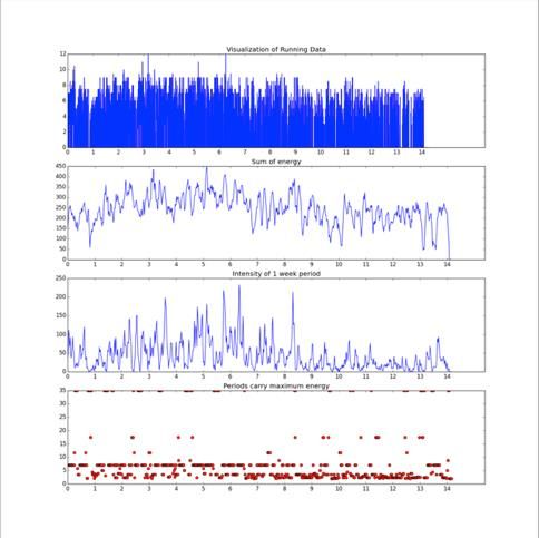
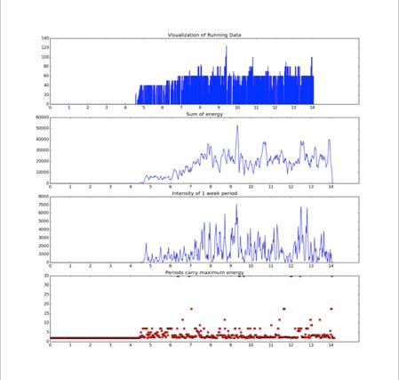
FP7-288199
D4.5 – Activity Monitoring and Lifelogging v2

5.2 Pattern Discovering in Lifelog Data ....................................................................... 52
 5.2.1 Periodicity Detection ........................................................................................................ 52
 5.2.2 Periodicity Methodology .................................................................................................. 52
 5.2.3 Intensity of Periods .......................................................................................................... 54
 5.2.4 Dataset (Periodicity) ......................................................................................................... 55
5.3 Results ..................................................................................................................... 58
 5.3.1 Periodogram..................................................................................................................... 58
 5.3.2 Intensity of Periodogram .................................................................................................. 62
 5.3.3 Conclusions ..................................................................................................................... 65
5.4 References ............................................................................................................... 66

 INTEGRATION OF COMPONENTS AND USAGE IN PILOTS ...................... 67

 CONCLUSIONS .......................................................................................... 70

 Page 7

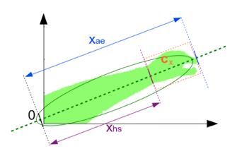
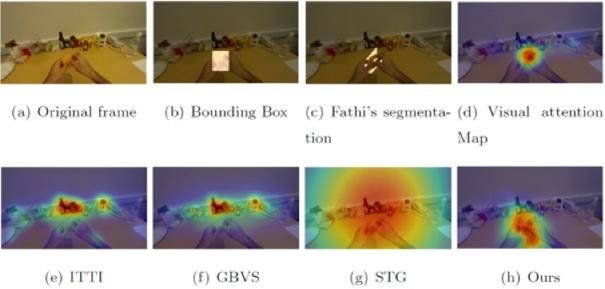
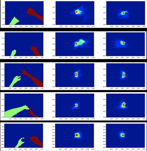
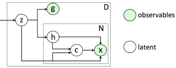
FP7-288199
D4.5 – Activity Monitoring and Lifelogging v2

List of Figures
Figure 2-1: (a) Bi-partite graph with hypothetical associations. (b) Associations of trajectories
from each camera after Hungarian algorithm is applied. ....................................................... 13
Figure 2-2: (a) The optimal warping path. (b) DTW results for tracklet 1 of two trajectories
comparison. In X and Y the frames are shown. The optimal path is represented in green, and
the DTW result is shown in red. ............................................................................................ 14
Figure 2-3: (a) The doctor and patient projections from the left view to the right. (b) Patient
trajectories from mono-view and after merging. (c) Doctor trajectories from mono-view and
after merging. ....................................................................................................................... 16
Figure 3-1: 3D Localization From Wearable Camera Problem .............................................. 19
Figure 3-2: Workflow of the proposed large-scale 3D reconstruction framework .................. 20
Figure 3-3: Sub-map reconstruction framework .................................................................... 21
Figure 3-4: Superimposed reconstructed camera trajectory (blue line) with the ground plan of
the flat. ................................................................................................................................. 22
Figure 3-5: Localization framework ...................................................................................... 23
Figure 3-6: Sequence 1 - Superimposed estimated camera trajectory (blue line) with the
ground truth (red line). ..........................................................................................................25
Figure 3-7: Sequence 2 - Superimposed estimated camera trajectory (blue line) with the
ground truth (red line)...........................................................................................................25
Figure 3-8 Illustrations of the 6 global features. 1(a): Relative location of hands, 1(b): Left
arm orientation, 1(c): Left arm depth and Right arm depth with regard to the camera. ...........28
Figure 3-9 Representation of the arm segmentations closest to the centre of 8 global
appearance model clusters. Each cluster is represented by the sample that is closest to the
cluster centre. ....................................................................................................................... 29
Figure 3-10 Illustration of the hand centre c computed as the barycentre of the orange box and
the key points around: xhs the starting position of the hand on the major ellipse axis, and xae
the end position of the whole arm. ........................................................................................ 29
Figure 3-11 Graph representing the ratio between hands beginning and arm length depending
on the minor/major axis lengths of the ellipse fitting the segmented arms. Blue dots
correspond to the values manually annotated, red line to the fitting exponential model ......... 30
Figure 3-12 Graphical model of our approach Top-down visual attention modelling with
manipulated objects. Nodes represent random variables (observed-shaded, latent-unshaded),
edges show dependencies among variables, and boxes refer to different instances of the same
variable................................................................................................................................. 31
Figure 3-13 Five examples of the obtained experimental distributions p |h = j, , zk. Left
column: arm segmentation closest to cluster, Middle column: left hand distribution, Right
column: right hand distribution. ............................................................................................ 33
Figure 3-14 Saliency models selected for comparison. .......................................................... 35

 Page 8

FP7-288199
D4.5 – Activity Monitoring and Lifelogging v2

Figure 3-15 Object recognition performances between different paradigms. The results are
given in average precision per category and averaged. .......................................................... 38
Figure 3-16 Object recognition performances between different saliency models applied to the
saliency weighted BoVW paradigm. The results are given in AP per category and averaged. 39
Figure 4-1 Dem@Care lab experiments: From left to right and top to bottom Dem@Care1:
Eat Snack, Enter Room, HandShake, Read Paper, Dem@Care2: Serve Beverage, Start
Phonecall, Drink Beverage and HandShake, Dem@Care3: Prepare Drug Box, Prepare Drink,
Turn On Radio, Water Plant. Dem@Care4: Answer phone, Prepare Drug Box, Prepare Hot
Tea, Establish Account Balance. ........................................................................................... 42
Figure 4-2 Dem@Care home experiments: From left to right and top to bottom
Dem@Home1:Wash Dishes, Prepare Meal, Eat. Dem@Home2:Sit on couch, Open fridge,
kitchen activity. .................................................................................................................... 43
Figure 5-1: Visualisation of raw sleep data ...........................................................................56
Figure 5-2: Visualization of raw data in the sports activity dataset ........................................ 57
Figure 5-3: Moving average values for sports dataset (Run, Cycle, Swim, Aggregated) ........ 58
Figure 5-4: Sleep duration periodogram ................................................................................ 59
Figure 5-5: Sleep quality periodogram .................................................................................. 59
Figure 5-6: Sports dataset periodograms ............................................................................... 60
Figure 5-7: Sports Dataset Autocorrelations (10-year span) .................................................. 60
Figure 5-8: Autocorrelation plots of sports data from year 2007............................................ 61
Figure 5-9: Periodogram of @Home pilot sleep data............................................................. 62
Figure 5-10: Intensity (Running data) ................................................................................... 63
Figure 5-11: Intensity (Swimming data)................................................................................ 64
Figure 5-12: Frequency carrying maximum energy (Dem@Care sleep data) ......................... 64
Figure 5-13: Intensity of 36-hour periodicity ........................................................................ 65

 Page 9

FP7-288199
D4.5 – Activity Monitoring and Lifelogging v2

List of Tables

Table 2.1: Mono and multi-camera tracking results for the right camera view for a video ..... 16
Table 2.2: Tracking results of the proposed approach and mono-camera tracking approach
resulting from left and right view for 5 videos ......................................................................17
Table 3.1 Validation of the number of global appearance models K ......................................35
Table 3.2 NSS mean scores (with standard deviations) between human points and different
saliency map models. ............................................................................................................ 36
Table 4.1 Activity Recognition Accuracy for 640x480 resolution, with block matching
speedup ................................................................................................................................ 45
Table 5.1: MET table ............................................................................................................ 56

 Page 10

FP7-288199
D4.5 – Activity Monitoring and Lifelogging v2

 Introduction

The central objective of WP4 is to analyse audio-visual recordings of people with dementia so
as to recognise activities and situations of interest, assess their mental and emotional state and
extract behavioural and lifestyle profiles, trends, and alarms. The activities of interest and the
assessment of the individuals’ status are based on the clinical requirements described in D2.2
and system functional requirements presented in D7.1. The outcomes of the audio-visual
situational analysis will be fused with the other sensor data for a comprehensive picture of the
person’s condition and its progression, and will be critical in designing and implementing the
optimal approach for personalised care.
Deliverable D4.5 includes the description of the final version of Dem@Care tools for
analysing visual data and their evaluation on the datasets obtained during data acquisition
within Dem@Care. The visual analytics aim at posture recognition, action recognition,
activity monitoring, life-logging. D4.5 extends deliverable D4.2, which presented a study of
the state of the art and a description of the first set of tools, by improving upon the methods
presented in it, and expanding the experimental evaluation.

D4.5 consists of 4 main chapters, following the structure of D4.2.
Chapter 2 describes the research conducted for tracking individuals through a scene using
multiple cameras, and shows how the proposed approach improves upon state of the art
algorithms for single camera tracking.
Chapter 3 presents the research carried out on video analysis for Action Recognition through
Object Recognition and Room Recognition on video data from a wearable camera.
Chapter 4 describes the methods developed for Activity Recognition and Person Detection
from video and RGB-D cameras, as well as their results on real-world recordings.
Chapter 5 presents Periodicity Detection on longitudinal lifelog data where signal analysis
techniques are used to identify routines and periodic behaviour of an individual.
Chapter 6 presents a holistic component integration and pilot usage section, which
summarizes all WP4 research and development contributions to real-world piloting, as well as
the clinical results in the context of Dem@Care.

 Page 11

FP7-288199
D4.5 – Activity Monitoring and Lifelogging v2

 People Tracking for Overlapped Multi-cameras

2.1 Introduction
People-tracking plays an important role for activity recognition, as it allows to disambiguate
between different individuals in the same scene, so as to correctly recognize the activities they
are carrying out. In Dem@Care we install several cameras so as to completely cover the scene
under consideration. In this deliverable, a new tracking approach using data from multiple
cameras is presented. We evaluate the proposed method on the Dem@Care data and compare
its results with a mono-camera tracking algorithm. The comparison shows a considerable
improvement of tracking performance while using the proposed approach.

2.2 Proposed Multi-camera Tracking Approach

2.2.1 Description of the Proposed Approach
This approach comprises of three steps: mono-camera tracking, trajectory association and
trajectory merging. The objective of mono-camera tracking is to compute the trajectories of
each person in the scene, corresponding to each camera viewpoint. In the second step, we
search for the best matching for trajectories from one viewpoint to the other. In the last step,
after computing the best matching pairs, we compute the merged trajectories, taking into
account the reliability of trajectories extracted from the mono-view.

2.2.2 Mono-camera tracking
Object tracking from one camera relies on the computation of object similarity across
different frames using eight different object appearance descriptors: colour histogram, colour
covariance, 2D and 3D displacement, 2D shape ratio, 2D area, HOG and dominant colour.
Based on these descriptor similarities, the object similarity score is defined as a weighted
average of individual descriptor similarity. Trajectories are then computed as those
maximizing the similarities of the objects that belong to the same trajectory.

2.2.3 Trajectory Association
The association problem is related to the need for establishing correspondences between
pairwise similar trajectories that come from different cameras. The question is: which object,
visible from one camera, can be associated with which objects visible from the other cameras.
For two cameras, the association or correspondence may be modelled as a bi-partite matching
problem, where each set has trajectories that belong to each camera. Let Cl and Cr denote two
overlapping cameras. For each camera, a set of trajectories Sleft and Sright is defined. A bi-
partite graph G = (V; E) is a graph in which the vertex set V can be divided into two disjoint
subsets Sleft and Sright, such that every edge ∈ has one end point in Sleft and the other end
point in Sright.

 Page 12

FP7-288199
D4.5 – Activity Monitoring and Lifelogging v2

 (a) (b)
 Figure 2-1: (a) Bi-partite graph with hypothetical associations. (b) Associations of trajectories from
 each camera after Hungarian algorithm is applied.

Let represent the ith physical object that belongs to trajectory TrjCk observed by camera Ck, ,
where k = {l, r}, is the length of the trajectory j. Each trajectory is composed of a time
sequence of physical objects:
 = { 0 , 1 , … , , … , } (1)
Consequently, camera Cl and Cr have a set of trajectories of size N and M called Sright and Sleft :
 ℎ = { 0 , 1 , 2 , . . . , } (2)
 = { 0 , 1 , 2 , . . . , }
Once the bi-partite graph is built, we need to find pair-wise trajectories similarities. To
perform this task, we use spatial and temporal trajectory features. We transform the trajectory
association problem across multiple cameras as follows: each trajectory TrjCk is a node of the
bi-partite graph that belongs to set Sk for camera Ck . A hypothesized association between two
trajectories is represented by an edge in the bi-partite graph, as shown in Figure 2-1(a). The
goal is to find the best matching pairs in the graph.

Trajectory Similarity Calculation
There are several trajectory similarity measurements in the state of the art. We choose the
Dynamic Time Warping approach (DTW) [2.11] because it is conceptually simple and
effective for our trajectory similarity calculation. DTW is a dynamic-programming-based
technique with O(N 2 ) complexity, where N is the length of the trajectories to be compared.
Over the last years, several authors has been studying and applying this method [2.9, 2.12,
2.13].
The NxN grid is first initialized with values of infinity (∞) that represent infinite distances.
Each element (n, m) represent the Euclidean distance between two points TriCl (n), TrjCr (m)
∀n, m ∈ [0 … N] defined as follows:

 2 2 2 (3)
 ( ( ), ( )) = √( ( ) − ( ) ) + ( ( ) − ( ) )
 
where (x, y) is the 2D location of trajectories after projecting on a reference view.

 Page 13

FP7-288199
D4.5 – Activity Monitoring and Lifelogging v2

 (a) (b)

 Figure 2-2: (a) The optimal warping path. (b) DTW results for tracklet 1 of two trajectories
comparison. In X and Y the frames are shown. The optimal path is represented in green, and the DTW
 result is shown in red.

Many paths connecting the beginning and the ending point of the grid can be constructed. The
goal is to find the optimal path that minimizes the global accumulative distance between both
trajectories.
From the DTW results, we build a cost matrix with a normalized Euclidean Distance Mean
based metric for each trajectory pair. In order to normalize the distance values computed by
DTW, we divide a distance value by the maximum possible distance between two trajectories
which is the diagonal of the image:
 ( , ) (3)
 ( , ) =
 2 2
 √( ( ℎ ) + ( ℎ )2 )

Now the bi-partite graph is complete and the weight of each edge in = ( ; ) is given
by EDM(i, j) (Figure 2-1(a)). The task at hand now consists in finding the optimal matching
of , aimingto find the optimal assignment that maximizes the total cost of a matrix. To find
the optimal matching in we apply the Hungarian Algorithm defined by Kuhn [2.15], given
the cost matrix built with the values. The Hungarian method is a combinatorial
optimization algorithm that solves the assignment problem in polynomial time ( 3 ), where
 is number of nodes or vertexes of the bi-partite graph . After apply the Hungarian
Algorithm to the matrix we got the maximum matching as is shown in Figure 2-1(b).
2.2.4 Trajectory Merging
Once association is done, the next step is to compute the final trajectory by merging
corresponding trajectories from each view. To merge two trajectories coming from two
different cameras, e.g. ∈ ℎ ℎ 0 < < and ∈ ℎ 0 < < into a
global one TrGij , we apply an adaptive weighting method as follows:
 1 1 ( ) + 2 2 ( ) 1 ( ), 2 ( ) ∃ (4)
 , ( ) = { 1 ( ) 1 ( ) ∃ ^ 2 ( ) ∄ 
 2 ( ) 2 ( ) ∃ ^ 1 ( ) ∄ 

 Page 14

FP7-288199
D4.5 – Activity Monitoring and Lifelogging v2

As we defined in Eq. (3), each trajectory is composed by a set of detections. Chau et al. [2.1]
defined a method to quantify the reliability of the trajectory of each interest point by
considering the coherence of the Frame-to-Frame (F2F) distance, the direction, and the HOG
similarity of the points belonging to a same trajectory. Thus, as each physical object has
reliability attribute with values [0, 1]. The weight of each trajectory is defined in term of its
R-value as follows:
 (5)
 1 = 2 =
 + + 
It is important to note that w1 + w2 = 1. The merged trajectory is located in between the two
cameras from mono-view, and is closer to the trajectory with higher reliability values.

2.3 Discussion and results
The objective of this evaluation is to prove the effectiveness of the proposed approach, and to
compare it with a mono-camera tracking. We select five videos from the Dem@Care dataset
recorded in the Centre Hospitalier Universitaire Nice (CHUN) hospital, which involved
participants with dementia over 65 years old. Experimental recordings used two widely
separated RGB-D cameras (Kinect®, Microsoft©) with 640x480 pixel resolution, recording
between 6 and 9 frames per second. Each pair of videos has two different views of the scene,
lateral, and frontal, with two people per view, the person with dementia and the doctor. They
sometime cross each other or are hidden behind furniture. They exit the scene and re-enter it
several times.
Figure 2-3(a) shows two camera views of the scene. The blue lines represent the trajectory
projection from the left camera to the right camera, which has been selected as reference.
After the whole video is processed, we obtain the trajectories association and fusion for the
doctor and patient trajectories. In Figure 2-3(b) the trajectory ( , ) in terms of the time (in
frames) is presented. The yellow is the final patient trajectory, which is in between the right
camera trajectory, and the projection of the left camera trajectory. Figure 2-3(c) presents the
doctor’s trajectory with the same colour annotation.
In order to quantify our results, we use the tracking time-based metrics from [2.18]. The
tracking results are compared against entire trajectories of ground truth data. This metric gives
us a global overview of the performance of the tracking algorithm. In this section we present
the overall evaluation of our multi-camera tracking approach and its comparison with the
mono-camera tracking algorithm [2.1].

Table 2.1 presents the tracking results of the proposed approach and mono-camera tracking
approach resulting from the right viewpoint of a video. Our multi-camera tracking approach
provides much better performance compared to the mono-camera tracking approach. Tracking
time increases 20.79% for the first trajectory (doctor), and 6.41% for the second one (patient).

 Page 15

FP7-288199
D4.5 – Activity Monitoring and Lifelogging v2

 (a)

 (c )
 (b)
 Figure 2-3: (a) The doctor and patient projections from the left view to the right. (b) Patient
 trajectories from mono-view and after merging. (c) Doctor trajectories from mono-view and after
 merging.

 Table 2.1: Mono and multi-camera tracking results for the right camera view for a video

 Approaches Camera view Object 1 (Doctor) Object 2 (Patient)
 Tracking time Tracking time
Mono-camera tracker Right 49,67% 86,31%
Our multi-camera tracker Left and Right 70,45% 92,72%

Table 2.1 presents the tracking results of the proposed approach and mono-camera tracking
approach resulting from the left and right views of 5 videos (10 people in total). We achieved
considerably better performance than the mono-camera tracking algorithm of [2.1]. The multi-
camera tracking approach outperforms the mono-camera results for both camera views. For
the doctor’s trajectory, the most significant improvement is against the right camera
viewpoint’s result, which is surpassed by 19.67%. In the case of the patient’s trajectory the
best results (an improvement of 25.5%) are achieved compared to the results from the left
camera viewpoint. For the person with dementia we achieved a high tracking time, of 91.3%,
but only 66.92%for the doctor trajectory, which can be attributed to misdetection of the doctor
from both viewpoints.

 Page 16

FP7-288199
D4.5 – Activity Monitoring and Lifelogging v2

 Table 2.2: Tracking results of the proposed approach and mono-camera tracking approach resulting
 from left and right view for 5 videos

 Approaches Camera view Object 1 (Doctor) Object 2 (Patient)
 Tracking time Tracking time
 Mono-camera tracker Right 47,24% 85,21%
 Mono-camera tracker Left 52,76% 65,79%
 Our multi-camera tracker Left and Right 66,92% 91,30%

2.4 Conclusion
We have presented a novel multi object tracking process for multiple cameras. For each
camera, tracking by detection is performed. Trajectory similarity is computed using a
Dynamic Time Warping approach. Afterwards, the association of trajectories takes place as a
maximum bi-partite graph matching, addressed by the Hungarian algorithm. Finally, the
merging processes between associated trajectories has taken place with an adaptive weighting
method.

We evaluate the multi-camera approach in a real-world scenario and compare its results to the
mono-camera approach. Our method considerably outperforms the mono-camera tracking
algorithm [2.1], with good occlusion management and providing more complete trajectories
by recovering additional information, which is not available in a single view. In future work,
we will modify this algorithm to achieve online processing.

2.5 References
[2.1] D. P. Chau, F. Bremond, and M. Thonnat, “A multi-feature tracking algorithm
 enabling adaptation to context variations,” The International Conference on Imaging
 for Crime Detection and Prevention (ICDP), 2011. [Online]. Available:
 http://arxiv.org/pdf/1112.1200v1.pdf. [Accessed: 25-Apr-2014].
[2.2] N. Anjum and A. Cavallaro, “Trajectory Association and Fusion across Partially
 Overlapping Cameras,” 2009 Sixth IEEE Int. Conf. Adv. Video Signal Based
 Surveill., 2009.
[2.3] Y. A. Sheikh and M. Shah, “Trajectory association across multiple airborne cameras.,”
 IEEE Trans. Pattern Anal. Mach. Intell., vol. 30, pp. 361–367, 2008.
[2.4] T.-H. Chang and S. Gong, “Tracking multiple people with a multi-camera system,”
 Proc. 2001 IEEE Work. Multi-Object Track., 2001.
[2.5] S. M. Khan and M. Shah, “A Multiview Approach to Tracking People in Crowded
 Scenes Using a Planar Homography Constraint,” Comput. Vision–ECCV 2006, vol.
 3954, pp. 133–146, 2006.
[2.6] R. Eshel and Y. Moses, “Homography based multiple camera detection and tracking
 of people in a dense crowd,” 2008 IEEE Conf. Comput. Vis. Pattern Recognit., 2008.
[2.7] Richard Hartley and Andrew Zisserman, Multiple View Geometry in Computer
 Vision. Cambridge university press, 2003.

 Page 17

FP7-288199
D4.5 – Activity Monitoring and Lifelogging v2

[2.8] A. Yilma and M. Shah, “Recognizing human actions in videos acquired by
 uncalibrated moving cameras,” Tenth IEEE Int. Conf. Comput. Vis. Vol. 1, vol. 1,
 2005.
[2.9] Peng Chen, Junzhong Gu, Dehui Zhu, Fei Shao, “A Dynamic Time Warping based
 Algorithm for Trajectory Matching in LBS,” Int. J. Database Theory Appl., vol. Vol.
 6, no. Issue 3, pp. p39–48. 10p., 2013.
[2.10] L. Bergroth, H. Hakonen, and T. Raita, “A survey of longest common subsequence
 algorithms,” Proc. Seventh Int. Symp. String Process. Inf. Retrieval. SPIRE 2000,
 2000.
[2.11] A. Kassidas, J. F. Macgregor, and P. A. Taylor, “Synchronization of batch trajectories
 using dynamic time warping,” AIChE J., vol. 44, pp. 864–875, 1998.
[2.12] H. J. Ramaker, E. N. M. Van Sprang, J. A. Westerhuis, and A. K. Smilde, “Dynamic
 time warping of spectroscopic BATCH data,” Anal. Chim. Acta, vol. 498, pp. 133–
 153, 2003.
[2.13] Y. Z. Y. Zhang and T. F. Edgar, “A robust Dynamic Time Warping algorithm for batch
 trajectory synchronization,” 2008 Am. Control Conf., 2008.
[2.14] T. Kashima, “Average trajectory calculation for batch processes using Dynamic Time
 Warping,” SICE Annu. Conf. 2010, Proc., 2010.
[2.15] H. W. Kuhn, “The Hungarian Method for the Assignment Problem,” 50 Years Integer
 Program. 1958-2008, pp. 29–47, 2010.
[2.16] K. Bernardin and R. Stiefelhagen, “Evaluating Multiple Object Tracking Performance:
 The CLEAR MOT Metrics,” EURASIP J. Image Video Process., vol. 2008, pp. 1–10,
 2008.
[2.17] Y. Li, C. Huang, and R. Nevatia, “Learning to associate: HybridBoosted multi-target
 tracker for crowded scene,” 2009 IEEE Conf. Comput. Vis. Pattern Recognit., 2009.
[2.18] A. T. Nghiem, F. Bremond, M. Thonnat, and V. Valentin, “ETISEO, performance
 evaluation for video surveillance systems,” in Advanced Video and Signal Based
 Surveillance, 2007. AVSS 2007. IEEE Conference on, 2008, pp. 476–481.

 Page 18

FP7-288199
D4.5 – Activity Monitoring and Lifelogging v2

 Action Recognition

3.1 3D Localization From Wearable Camera

In this work, we are interested in estimating the position of a patient moving in an apartment
from a wearable camera (see Fig. 3-1). To achieve this, we first develop a complete 3D
reconstruction framework to robustly and accurately reconstruct a whole apartment from a
training video. Then, we propose a localization approach that relies on the 3D model of the
environment to estimate the position of the camera from a new video.

 Figure 3-1: 3D Localization From Wearable Camera Problem

3.1.1 Reconstruction of an apartment from a wearable camera
In D4.3 we presented a 3D reconstruction framework that is able to estimate both the camera
pose, as well as a sparse 3D point cloud from a few hundred images of a single room.
However, when the number of images increases, the computational complexity of the
approach quickly becomes prohibitive. Thus the previously proposed framework can only
reconstruct a room and not a whole apartment. Here, we are interested in building a globally
consistent 3D model of an entire apartment.

Our new large-scale 3D reconstruction framework builds upon the framework introduced in
the previous deliverable. It also deals with videos and thus takes advantage of the temporal
continuity of the video frames, while the previous framework assumed that the frames where
unordered. The workflow of the proposed approach is illustrated in Figure 3-2.

 Page 19

FP7-288199
D4.5 – Activity Monitoring and Lifelogging v2

 Figure 3-2: Workflow of the proposed large-scale 3D reconstruction framework

3.1.2 Keyframe Selection
First of all, our approach selects keyframes among all the video frames by running a Lucas-
Kanade tracker on the frames. It works as follows:
 [1] The first video frame is a keyframe.
 [2] Iterate until the end of the video
 [1] Set next video frame as current frame
 [2] Run the Lucas-Kanade tracker
 [3] If the distance between the 2D points tracked in the previous keyframe and the 2D
 points matched to them in the current frame is higher than a threshold (typically 10%
 of the width of a frame) then set the current frame as a keyframe
 [4] Go to 1
This keyframe selection allows us to take advantage of the temporal continuity of the video
frames by tracking features between keyframes instead of simply trying to match features
between keyframes.

3.1.3 Sub-map Reconstruction
After having selected keyframes, we define overlapping subsets of consecutive keyframes.
For each subset of keyframes, we estimate a sub-map, i.e a 3D point cloud as well as the
camera poses, with a framework similar to the one described in the previous deliverable. The
workflow of the sub-map reconstruction framework is illustrated in Figure 3-3. The main
modification with respect to the previous deliverable relies in the modification of the “global
camera orientation estimation” where we now employ an iterated extended Kalman filter on
Lie groups (accepted in ICIP 2014). Further details on this sub-map reconstruction framework
have been submitted to CVPR 2015 and will be available soon.

 Page 20

FP7-288199
D4.5 – Activity Monitoring and Lifelogging v2

 Figure 3-3: Sub-map reconstruction framework
3.1.4 Relative Similarity Averaging
Once all the sub-maps have been estimated, we need to align them to obtain a globally
consistent 3D model. Aligning these sub-maps consists in computing and averaging relative
3D similarities (scale, rotation and translation) between them.
To compute the relative similarities, we propose the following approach:
 For each point cloud:
  Select the 3D points that have a “small ” covariance.
  Compute a signature. We use a bag of visual words approach and consider the
 histogram as a signature.
  Find the 100 “closest” point clouds. Here “closest” means w.r.t the L2 distance
 between signatures.
  Match the 3D point descriptors of each of these point clouds to the 3D points
 descriptors of the current point cloud.
  Compute the relative 3D similarities between the best 30 point clouds and the
 current point cloud by minimizing the distances between the matched 3D points.
 If two sub-maps are overlapping, i.e. if they share cameras, then we also include
 the distance between these cameras poses in the criterion. In this step, a RANSAC
 algorithm is applied since matches between 3D points usually produces outliers.
Once that all relative 3D similarities have been computed, we need to average them. To do so,
we apply the iterated extended Kalman filter on Lie groups (that was accepted in ICIP 2014).
Unfortunately, this algorithm is not robust to outlier measurements while the relative 3D
similarities might contain outliers. Indeed, two point clouds representing two places from
different rooms that have a similar geometry might produce a relative similarity measurement.
In order to deal with these outliers, we apply a robust approach, still based on the iterated
extended Kalman filter on Lie groups that was accepted in ACCV 2014.
As we will see in the next section, this approach is able to efficiently reject outliers, while
aligning the sub-maps to obtain a globally consistent 3D model.

3.1.5 Qualitative Results
We qualitatively evaluate the performance of our system on a video sequence of 10000
frames recorded in an apartment. Our framework currently runs in Matlab and took 2.5 hours

 Page 21

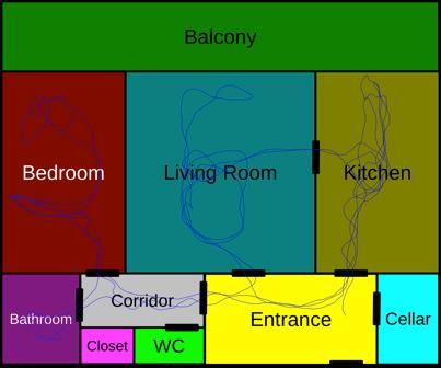
FP7-288199
D4.5 – Activity Monitoring and Lifelogging v2

to process the training video. Even if this is already a reasonable computation time, it could be
significantly reduced using C/C++. After having applied our automatic framework to the
video sequence, we obtained a set of aligned sub-maps, with each sub-map containing a 3D
point cloud and part of the camera trajectory. In order to qualitatively evaluate the result, we
manually place the estimated camera trajectory from the training video sequence on top of the
ground plan of the flat (see Figure 3-4). As it can be seen, the superimposed camera trajectory
is coherent with the ground plan, i.e it trajectory goes into (almost) every room without
crossing the walls and passes through the doors when going from one room to another.

Figure 3-4: Superimposed reconstructed camera trajectory (blue line) with the ground plan of the flat.

3.1.6 Metric Localization from a wearable camera
In the previous section, we presented a new algorithm to reconstruct a 3D model of an entire
apartment from a training video. We now propose a localization framework that relies on this
3D model to estimate the position of the camera from a new video. This new localization
algorithm employs two different place detectors. The first place detector is based on the
appearance of the scene, which provides robustness to motion blur and moving objects. The
second detector is based on the 3D geometry of the model, which makes it highly accurate but
not always available. The result of both detectors are fused using a novel Rao-Blackwellized
particle filter on the Lie group SE(3) that relies on a white noise acceleration model to
produce the final camera trajectory. The proposed framework is presented in Figure 3-5.

 Page 22

FP7-288199
D4.5 – Activity Monitoring and Lifelogging v2

 Figure 3-5: Localization framework

Keyframe Selection
In order to reduce the number of frames to localize, we perform keyframe selection over the
video frames to only keep the frames where the person is actually moving. This keyframe
selection step is the same as the one depicted in the previous section.

SURF points detection
After having selected keyframes, SURF points are extracted. These points will be used both
by the appearance based place detector and the 3D based place detector.

Appearance based place detection
For each keyframe of the 3D model previously reconstructed, we have saved its SURF points,
a 32x32 miniature as well as its position and orientation w.r.t the 3D point cloud. The aim of
this module is to exploit the information, that we call the “appearance” of the 3D model, to
localize each keyframe of the new video. Here, we do not use the reconstructed 3D point
cloud.

We now detail how a keyframe K of the new video is localized.
First of all, a 32x32 miniature is created and compared to the miniatures of the 3D model
using the L1-norm. Then, the 100 closest keyframes of the 3D model are re-ranked by
matching their SURF points to those of K using kd-trees and bi-directional matching.
Finally, from the 10 closest keyframes of the 3D model, a mixture of Gaussian distributions is
created where the mean of each component is set as the pose of the corresponding keyframe,
the covariance is defined by hand (each component has the same covariance) and the weight
is proportional to the number of matches. This mixture of Gaussians will be used by the Rao-
Blackwellized particle filter.

3D based place detection
The aim of this module is to exploit the reconstructed 3D point cloud to localize each
keyframe of the new video.
To do so, for a keyframe K, we first match its SURF points to the SURF points of the 3D
model. We then apply a PnP algorithm combined with a RANSAC to robustly estimate the
pose of K. Based on a Gauss-Newton algorithm, the estimated pose is finally refined by
minimizing the reprojection error of the 3D points in the keyframe. Around the estimated

 Page 23

FP7-288199
D4.5 – Activity Monitoring and Lifelogging v2

pose, the covariance matrix of the estimated errors is approximated by performing a Laplace-
like approximation.
To increase the performances of this 3D based detector, the described method is actually
applied to the point cloud of each sub-map.
The output of this detector is thus once again a mixture of Gaussian distributions that will be
used by the Rao-Blackwellized particle filter.

Rao-Blackwellized Particle Filter on SE(3)
The aim of this module is to fuse the information coming from the appearance-based place
detector, which is robust to motion blur and moving objects, and the 3D based place detector
which is highly accurate but not always available, to reliably estimate the camera trajectory.
At each time instant, a mixture of Gaussian distributions (from the two place detectors) is
provided to the filter to select the “true” component. To do so, the filter employs
spatiotemporal a priori information, which states that camera poses should be close to each
other for two consecutive time instants. We use a white noise acceleration motion model to
represent this a priori information.
Consequently, at each time instant, the filter estimates the component of the mixture to select
as well as the pose of the camera (and its speed).
The discrete part of the state (the component selection) is sampled while the continuous part
(camera pose and speed) is solved analytically using an iterated extended Kalman filter on Lie
groups (ICIP 2014).

Qualitative and quantitative results
In order to evaluate the proposed localization framework, we recorded several videos in the
apartment that we previously reconstructed and manually built ground truth trajectories. Then
we applied the proposed localization framework to estimate camera trajectories. In Figures 3-
6 and 3-7, estimated camera trajectories and ground truth trajectories are represented for two
sequences. In the following table, the average position error is represented for these videos.
 Sequence 1 Sequence 2
Average Position Error (m) 0.54 0.64
One can see, that for those two videos, the camera trajectory is accurately estimated. The
current Matlab implementation achieves 1.3 FPS.

 Page 24

FP7-288199
D4.5 – Activity Monitoring and Lifelogging v2

 Figure 3-6: Sequence 1 - Superimposed estimated camera trajectory (blue line) with the ground truth
 (red line).

 Figure 3-7: Sequence 2 - Superimposed estimated camera trajectory (blue line) with the ground truth
 (red line)

3.1.7 Conclusion and Future Work
In this work, we first presented a complete 3D reconstruction framework able to robustly and
accurately reconstruct a whole apartment from a training video. Then, we proposed a
localization approach that relies on the 3D model of the environment to estimate the position
of the camera from a new video. We demonstrated, both qualitatively and quantitatively, that
the proposed localization framework was able to accurately estimate the camera trajectory
from a new video in an apartment previously reconstructed with the proposed 3D

 Page 25

FP7-288199
D4.5 – Activity Monitoring and Lifelogging v2

reconstruction framework. As future work, we are interested in cases where the place
detectors fail, for example when someone puts their hand in front of the camera.

3.2 Object recognition
3.2.1 Objectives
For the task of the assessment and life-logging of Alzheimer patients in their Instrumental
Activities of Daily Living (IADLs), egocentric video analysis has gained strong interest as it
allows clinicians to monitor patients’ activities and thereby study their condition and its
evolution and/or progression over time. Recent studies demonstrated how crucial the
recognition of manipulated objects is for activity recognition under this scenario [3.1, 3.2].
As described in earlier deliverables D4.1, D4.3, D4.4, visual saliency is an efficient way to
drive the scene analysis towards areas ‘of interest’ and has become very popular among the
computer vision community. Manipulated object recognition tasks can greatly benefit from
visual attention maps both to reduce the computational burden and filter out the most relevant
information.
Generally speaking, two types of attention are commonly distinguished in the literature:
bottom-up or stimulus-driven and top-down attention or goal-driven [3.3, 3.4]. The authors of
[3.3] define the top-down attention as the voluntary allocation of attention to certain features,
objects, or regions in space. They also state that attention is not only voluntary directed as
low-level salient stimuli can also attract attention, even though the subject had no intention to
attend these stimuli. A recent study [3.5] about how saliency maps are created in the human
brain, shows that an object captures our attention depending both on its bottom-up saliency
and top-down control.
Modelling of human visual attention has been an intensively explored research subject since
the last quarter of the 20th century and nowadays the majority of saliency computation
methods are designed from a bottom-up perspective [3.6]. Bottom-up models are stimulus-
driven, mainly based on low-level properties of the scene such as color, gradients orientation,
motion or even depth. Consequently, bottom-up attention is fast, involuntary and, most likely
feed-forward [3.6].
However, although the literature concerning models of top-down attention is clearly less
extensive, the introduction of top-down factors (e.g., face, speech and music, camera motion)
into the modelling of visual attention has provided impressive results in previous works [3.7,
3.8]. In addition, some attempts in the literature have been made to model both kinds of
attention for scene understanding in a rather “generic” way. In [3.9] the authors claim that the
top-down factor can be well explained by the focus in image, as the producer of visual content
always focuses his camera on the object of interest. Nevertheless, it is difficult to admit this
hypothesis for expressing the top-down attention of the observer of the content: it is always
task-driven [3.6].
More recent works using machine learning approaches to learn top-down behaviours based on
eye-fixation or annotated salient regions, have proven also to be very useful for static images
[3.10, 3.11, 3.12] as well as for videos [3.13, 3.14]. Furthermore, with advent of Deep
Learning Networks (DNN), some novel approaches have been designed in the field object
recognition, which build class-agnostic object detectors to generate candidate salient
bounding-boxes which are then labelled by later class-specific object classifiers [3.15, 3.16].
However, it seems impossible for us to propose a universal method for prediction of the top-
 Page 26

FP7-288199
D4.5 – Activity Monitoring and Lifelogging v2

down visual attention component, as it is voluntary directed attention and therefore it is
specific for the task of each visual search. Nevertheless, the prior knowledge about the task
the observer is supposed to perform, allows extracting semantic clues from the video content
that ease such a prediction.
The current state-of the art in computer vision allows for the detection of some categories of
objects with high confidence. A variety of face or skin detectors have been proposed in the
last two decades [3.17]. Hence, when modelling top-down attention in a specific visual search
task, we can use “easily recognizable” semantic elements that are relevant to the specific task
of the observer and may help to identify the real areas/objects of interest.
In this work we propose to use domain specific knowledge to predict top-down visual
attention in the task of recognizing manipulated objects in egocentric video content. In
particular, our “recognizable elements” (those relevant to the task) are the arms and hands of
the user wearing the camera and performing the action. Their quantized poses with regard to
different elementary components of a complex action such as object manipulation will help in
the definition of the area where the attention of the observer searching for manipulated objects
will be directed.
We evaluate our model from two points of view: i) prediction strength of gaze fixations of
subjects observing the content with the goal of recognition of a manipulated object, and ii)
performance in the target object recognition by a machine learning approach.

3.2.2 Goal-oriented top-down visual attention model
Our new top-down model of visual attention prediction in the task of manipulated object
recognition relies on the detection and segmentation of some objects, considered as
references, that help locate the actual areas of interest in a scene, namely the objects being
manipulated. In our proposal, arms/hands are automatically computed for each frame using
the approach introduced by Fathi et al. [3.18].
We propose to build our model as a combination of two distinct sets of features: global and
local. The former describes the geometric configuration of the segmented arms, which are
clustered into a pre-defined set of states/configurations. This global information is used to
select one of the components in a mixture model. The second set, concerning the local
features, is then modelled using the specific distributions corresponding to the selected global
component.

Defining Global features
The features we propose are based on the geometry of arms in the camera field of view, which
is correlated with the manipulated objects’ size and position. An elliptic region in the image
plane approximates each arm, from the elbow to the hand extremity. Hence an ellipse is first
fitted to each segmented arm area and, then, several global features are defined, namely:

  Relative location of hands: Two features are extracted that encode the relative location
 of one hand with respect to the other (see Figure 3-8 (a)). To that end, and when taking
 the left hand centre as the origin of coordinates, the vector that joins the origin and the
 right hand is represented by means of its magnitude and phase . The

 Page 27