SCALING CARBON FLUXES FROM EDDY COVARIANCE SITES TO GLOBE: SYNTHESIS AND EVALUATION OF THE FLUXCOM APPROACH - MPG.PURE
←
→
Page content transcription
If your browser does not render page correctly, please read the page content below
Biogeosciences, 17, 1343–1365, 2020
https://doi.org/10.5194/bg-17-1343-2020
© Author(s) 2020. This work is distributed under
the Creative Commons Attribution 4.0 License.

Scaling carbon fluxes from eddy covariance sites to globe:
synthesis and evaluation of the FLUXCOM approach
Martin Jung1 , Christopher Schwalm2 , Mirco Migliavacca1 , Sophia Walther1 , Gustau Camps-Valls3 , Sujan Koirala1 ,
Peter Anthoni4 , Simon Besnard1,5 , Paul Bodesheim1,6 , Nuno Carvalhais1,7 , Frédéric Chevallier8 , Fabian Gans1 , Daniel
S. Goll9 , Vanessa Haverd10 , Philipp Köhler11 , Kazuhito Ichii12,13 , Atul K. Jain14 , Junzhi Liu1,15 ,
Danica Lombardozzi16 , Julia E. M. S. Nabel17 , Jacob A. Nelson1 , Michael O’Sullivan18 , Martijn Pallandt19 ,
Dario Papale20,21 , Wouter Peters22 , Julia Pongratz23,17 , Christian Rödenbeck19 , Stephen Sitch18 ,
Gianluca Tramontana20,3 , Anthony Walker24 , Ulrich Weber1 , and Markus Reichstein1
1 Department   of Biogeochemical Integration, Max Planck Institute for Biogeochemistry, 07745 Jena, Germany
2 Woods   Hole Research Center, Falmouth, MA 02540-1644, USA
3 Image Processing Laboratory (IPL), Universitat de València, Paterna, 46980, Spain
4 Institute of Meteorology and Climate Research – Atmospheric Environmental Research (IMK-IFU),

Karlsruhe Institute of Technology, 82467 Garmisch-Partenkirchen, Germany
5 Laboratory of Geo-Information Science and Remote Sensing, Wageningen University and Research,

Wageningen, 6708 PB, the Netherlands
6 Computer Vision Group Mathematics and Computer Science, Friedrich Schiller University Jena, 07743 Jena, Germany
7 Departamento de Ciências e Engenharia do Ambiente (DCEA), Faculdade de Ciências e Tecnologia, FCT,

Universidade Nova de Lisboa, Caparica, 2829-516, Portugal
8 Laboratoire des Sciences du Climat et de l’Environnement (LSCE/IPSL), Université Paris-Saclay,

Gif-sur-Yvette, 91198, France
9 Department of Geography, University of Augsburg, 86159 Augsburg, Germany
10 Department Continental Biogeochemical Cycles, CSIRO Oceans and Atmosphere, Canberra, 2601, Australia
11 Division of Geological and Planetary Sciences, California Institute of Technology, Pasadena, CA, USA
12 Center for Environmental Remote Sensing (CEReS), Chiba University, Chiba, 263-8522, Japan
13 Center for Global Environmental Research, National Institute for Environmental Studies, Tsukuba, 305-8506, Japan
14 Department of Atmospheric Science, University of Illinois, Urbana, IL 61801, USA
15 School of Geography, Nanjing Normal University, Nanjing, 210023, China
16 Climate and Global Dynamics Laboratory, National Center for Atmospheric Research, Boulder, CO 80307, USA
17 Department Land in the Earth System (LES), Max Planck Institute for Meteorology, 20146 Hamburg, Germany
18 College of Life and Environmental Sciences, University of Exeter, Exeter, EX4 4QE, UK
19 Department of Biogeochemical Signals, Max Planck Institute for Biogeochemistry, 07745 Jena, Germany
20 Department of Innovation in Biology, Agri-food and Forest systems (DIBAF), Tuscia University, Viterbo, 01100, Italy
21 Impacts on Agriculture, Forests and Ecosystem Services (IAFES), Euro-Mediterranean Center on Climate

Change (CMCC), Lecce, 01100, Italy
22 Department of Meteorology and Air Quality, Wageningen University and Research, Wageningen, 6700 AA, the Netherlands
23 Department of Geography, Ludwig-Maximilians-Universität München, 80333 Munich, Germany
24 Climate Change Science Institute, Oak Ridge National Laboratory, Oak Ridge, TN, USA

Correspondence: Martin Jung (mjung@bgc-jena.mpg.de)

Received: 11 September 2019 – Discussion started: 2 October 2019
Revised: 29 January 2020 – Accepted: 30 January 2020 – Published: 16 March 2020

Published by Copernicus Publications on behalf of the European Geosciences Union.
1344                                                     M. Jung et al.: Synthesis and evaluation of the FLUXCOM approach

Abstract. FLUXNET comprises globally distributed eddy-               1   Introduction
covariance-based estimates of carbon fluxes between the
biosphere and the atmosphere. Since eddy covariance flux             Upscaling local eddy covariance (EC) measurements (Bal-
towers have a relatively small footprint and are distributed         docchi et al., 2001) from tower footprint to global wall-to-
unevenly across the world, upscaling the observations is             wall maps uses globally available predictor variables such as
necessary to obtain global-scale estimates of biosphere–             satellite remote sensing and meteorological data (Jung et al.,
atmosphere exchange. Based on cross-consistency checks               2011). These forcing data are first used to establish empir-
with atmospheric inversions, sun-induced fluorescence (SIF)          ical models for fluxes of interest at the site level and then
and dynamic global vegetation models (DGVMs), here we                to estimate gridded fluxes by applying these models across
provide a systematic assessment of the latest upscaling ef-          all vegetated grid cells. Previous FLUXNET upscaling ef-
forts for gross primary production (GPP) and net ecosystem           forts using machine learning techniques (Beer et al., 2010;
exchange (NEE) of the FLUXCOM initiative, where differ-              Jung et al., 2009, 2011) yielded global products that present
ent machine learning methods, forcing data sets and sets of          a data-driven “bottom-up” perspective on carbon fluxes be-
predictor variables were employed.                                   tween the biosphere and the atmosphere. These bottom-up
    Spatial patterns of mean GPP are consistent across FLUX-         products are complementary to process-based model sim-
COM and DGVM ensembles (R 2 > 0.94 at 1◦ spatial reso-               ulations and “top-down” atmospheric inversions. However,
lution) while the majority of DGVMs show, for 70 % of the            estimates of carbon fluxes are subject to uncertainty from
land surface, values outside the FLUXCOM range. Global               choice of machine learning algorithm and predictor vari-
mean GPP magnitudes for 2008–2010 from FLUXCOM                       ables, forcing data, FLUXNET measurements and incom-
members vary within 106 and 130 PgC yr−1 with the largest            plete representation of the different ecosystems therein. The
uncertainty in the tropics. Seasonal variations in indepen-          FLUXCOM initiative (http://www.fluxcom.org/, last access:
dent SIF estimates agree better with FLUXCOM GPP (mean               27 February 2020) aims to improve our understanding of the
global pixel-wise R 2 ∼ 0.75) than with GPP from DGVMs               multiple sources and facets of uncertainties in empirical up-
(mean global pixel-wise R 2 ∼ 0.6). Seasonal variations in           scaling and, ultimately, to provide an ensemble of machine-
FLUXCOM NEE show good consistency with atmospheric                   learning-based global flux products to the scientific commu-
inversion-based net land carbon fluxes, particularly for tem-        nity. Within FLUXCOM an intercomparison was conducted
perate and boreal regions (R 2 > 0.92). Interannual variability      for two complementary experimental setups of input drivers
of global NEE in FLUXCOM is underestimated compared                  and resulting global gridded products. These setups system-
to inversions and DGVMs. The FLUXCOM version which                   atically vary machine learning and flux partitioning meth-
also uses meteorological inputs shows a strong co-variation          ods as well as forcing data sets to separate measured net
in interannual patterns with inversions (R 2 = 0.87 for 2001–        ecosystem exchange (NEE) into gross primary productivity
2010). Mean regional NEE from FLUXCOM shows larger                   (GPP) and terrestrial ecosystem respiration (TER) (Jung et
uptake than inversion and DGVM-based estimates, particu-             al., 2019; Tramontana et al., 2016).
larly in the tropics with discrepancies of up to several hun-           Evaluating the strengths and weaknesses of the FLUX-
dred grammes of carbon per square metre per year. These              COM products and the approaches used therein is crucial to
discrepancies can only partly be reconciled by carbon loss           inform potential scientific uses and to guide future method-
pathways that are implicit in inversions but not captured by         ological developments. An evaluation based on site-level
the flux tower measurements such as carbon emissions from            cross-validation analysis (Tramontana et al., 2016) showed
fires and water bodies. We hypothesize that a combination            a general high consistency among machine learning algo-
of systematic biases in the underlying eddy covariance data,         rithms, experimental setups and flux partitioning methods
in particular in tall tropical forests, and a lack of site his-      applied in FLUXCOM. However, the conclusions from site-
tory effects on NEE in FLUXCOM are likely responsible for            level cross-validation may be limited by potential system-
the too strong tropical carbon sink estimated by FLUXCOM.            atic measurement errors that are inherent in the underlying
Furthermore, as FLUXCOM does not account for CO2 fer-                EC measurements (e.g. Aubinet et al., 2012) or the spa-
tilization effects, carbon flux trends are not realistic. Overall,   tially biased distribution of FLUXNET sites (Papale et al.,
current FLUXCOM estimates of mean annual and seasonal                2015). Therefore, cross-consistency checks of the FLUX-
cycles of GPP as well as seasonal NEE variations provide             COM products with independent estimates are important to
useful constraints of global carbon cycling, while interannual       consider. But such checks are complex due to limitations of
variability patterns from FLUXCOM are valuable but require           the independent approaches or the lack of comparability of
cautious interpretation. Exploring the diversity of Earth ob-        similar but not identical variables. In this study, we contextu-
servation data and of machine learning concepts along with           alize FLUXCOM products in relation to independent state-
improved quality and quantity of flux tower measurements             of-the-art estimates of carbon cycling. The comparison strat-
will facilitate further improvements of the FLUXCOM ap-              egy prioritizes robust features of the independent data sets
proach overall.                                                      and discusses residual uncertainties.

Biogeosciences, 17, 1343–1365, 2020                                                       www.biogeosciences.net/17/1343/2020/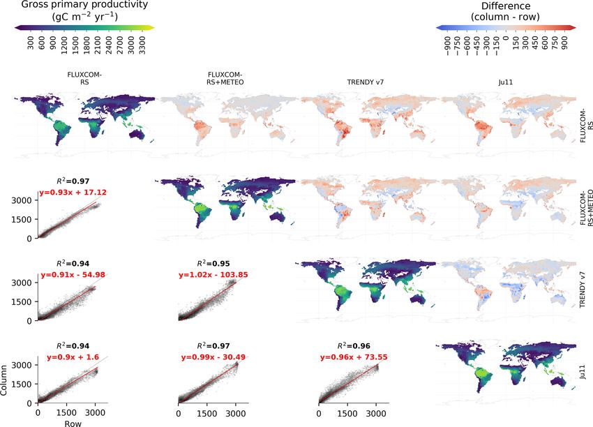
M. Jung et al.: Synthesis and evaluation of the FLUXCOM approach                                                             1345

Table 1. Global meteorological forcing data sets used in FLUXCOM-RS+METEO.

                             Meteorological forcing   Spatial resolution                     Temporal
                             data set                                                        coverage
                             CRU JRA                  0.5◦ × 0.5◦                            1950–2017
                             GSWP3                    0.5◦ × 0.5◦                            1950–2010
                             WFDEI                    0.5◦ × 0.5◦                            1979–2013
                             ERA-5                    0.5◦ × 0.5◦                            1979–2018
                             CERES–GPCP               1.0◦ × 1.0◦ resampled to 0.5◦ × 0.5◦   2001–2013

   The objectives of this paper are (1) to present a synthe-         chine learning methods with five global climate forcing data
sis and evaluation of FLUXCOM ensembles for GPP and                  sets (Table 1) yielded products with daily temporal and 0.5◦
NEE against patterns of remotely sensed sun-induced flu-             spatial resolution and time periods depending on the mete-
orescence (SIF) and atmospheric inversion results respec-            orological data. The meteorological data included WATCH
tively, (2) to discuss limitations of FLUXCOM and syn-               Forcing Data applied to ERA-Interim (WFDEI; Weedon
thesize lessons learned, and (3) to outline potential future         et al., 2014), Global Soil Wetness Project 3 forcing data
paths of FLUXCOM development. Due to limitations of the              (GSWP3, Kim, 2017), CRU JRA version 1.1 (Harris, 2019),
SIF product with respect to interannual variability (Zhang et        ERA5 (C3S, 2017), and a combination of observation-based
al., 2018), the evaluation of GPP against SIF is restricted          radiation from CERES (Doelling et al., 2013) and precipi-
to seasonal variations in photosynthesis. To reduce the im-          tation from GPCP (Huffman et al., 2001) (CERES–GPCP)
pact of atmospheric-transport-related uncertainties of inver-        resampled to 0.5◦ . The wide range of data sources from re-
sion products, mean annual and seasonal variations in NEE            analysis to station measurements to satellite observation is
are compared at regional scales while interannual variabil-          intentional and is meant to bracket potential uncertainties in
ity is assessed at a global scale. In addition, we contextualize     meteorological forcing.
our comparisons with FLUXCOM by providing comparisons                   For GPP and TER, we additionally considered uncertainty
with the previous model tree ensemble (MTE) results of Jung          from flux partitioning methods by propagating two different
et al. 2011 (Ju11) as well as an ensemble of process-based           variants, one based on night-time NEE data (Reichstein et
global dynamic vegetation model (DGVM) simulations from              al., 2005) and one on daytime data (Lasslop et al., 2010).
the TRENDY DGVM projects (Le Quéré et al., 2018; Sitch               Within the RS and RS+METEO setups, we followed a full
et al., 2015). Even though FLUXCOM also produced global              factorial design of machine learning methods (nine for RS,
products of TER, these are not shown here due to a lack of           three for RS+METEO), flux partitioning variants (two for
an independent observational benchmark.                              GPP and TER) and climate forcing input products (five, only
                                                                     for RS+METEO). Descriptions of machine learning meth-
                                                                     ods, training and validation setup are available in Tramon-
2     Data and methods                                               tana et al. (2016). The methodology of generating the global
                                                                     products is documented in detail in the overview paper on
2.1    FLUXCOM                                                       global energy fluxes from FLUXCOM (Jung et al., 2019).
                                                                        To allow for a better reuse of the large archive, we gener-
We used the cross-validated and trained machine learning             ated ensemble products of monthly values where individual
techniques for the FLUXCOM carbon fluxes of Tramon-                  ensemble members were first aggregated to monthly means
tana et al. (2016) and generated large ensembles (n = 120)           (Fig. 1). The ensemble products encompass estimates of
of global gridded flux products for two different setups: re-        different machine learning estimates, flux partitioning vari-
mote sensing (RS) and remote sensing plus meteorologi-               ants for GPP and TER, and different climate input data for
cal/climate forcing (RS+METEO) setups (Fig. 1). In the RS            RS+METEO. For the RS+METEO setup, this was also
setup, fluxes are estimated exclusively from Moderate Res-           done separately for each climate forcing data set to allow
olution Imaging Spectroradiometer (MODIS) satellite data.            modellers to compare their simulations with the FLUXCOM
In RS+METEO, fluxes are estimated from mean seasonal                 ensemble product driven by the same forcing. The ensem-
cycles of satellite data and daily meteorological informa-           ble products (hereafter referred to as FLUXCOM-RS and
tion (see Table S1 in the Supplement). For the rationale of          FLUXCOM-RS+METEO) were generated as the median
these setups, we refer the interested reader to Tramontana et        over ensemble members for each grid cell and month. The
al. (2016) and Jung et al. (2019). For the RS setup, nine ma-        FLUXCOM-RS products are based on nine ensemble mem-
chine learning methods were used to generate gridded prod-           bers for NEE and on 18 for GPP and TER. The FLUXCOM-
ucts at an 8 d temporal and 0.0833◦ spatial resolution for the
2001–2015 period. For the RS+METEO setup, three ma-

www.biogeosciences.net/17/1343/2020/                                                         Biogeosciences, 17, 1343–1365, 2020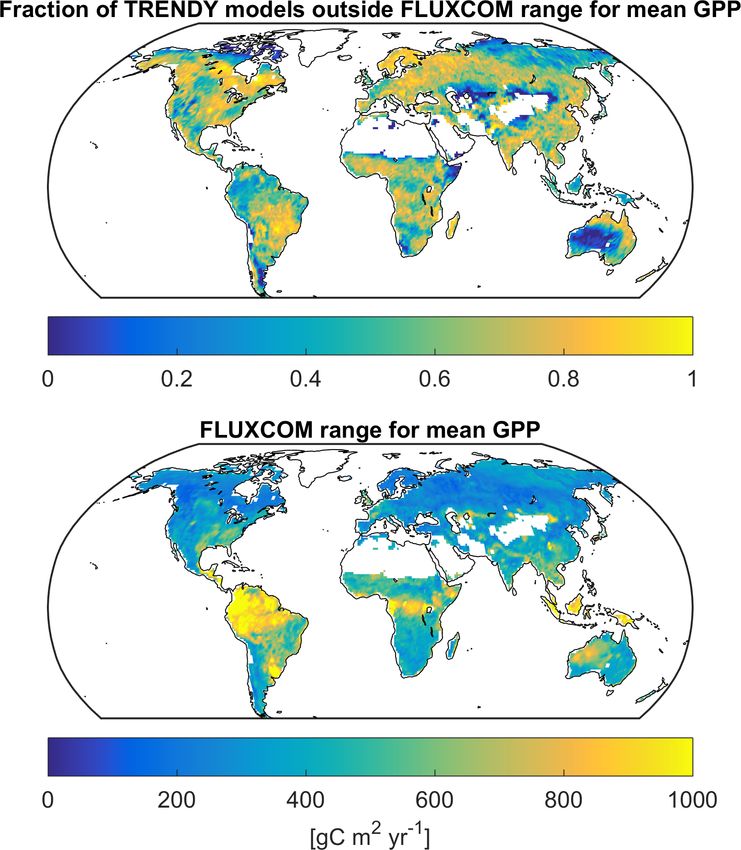
1346                                                     M. Jung et al.: Synthesis and evaluation of the FLUXCOM approach

Figure 1. Schematic overview of the methodology and data products from the FLUXCOM initiative. The flow diagram shows the method-
ological steps for the remote sensing (RS, left) and the remote sensing and meteorological data (RS+METEO, right) FLUXCOM products.
Final monthly ensemble products for NEE, GPP and TER from RS are available at 0.0833◦ and at 0.5◦ spatial resolution. Ensemble products
from RS+METEO are available per climate forcing (GC) data set as well as a pooled ensemble at 0.5◦ spatial resolution. All ensemble prod-
ucts encompass ensemble members of different machine learning methods (ML, nine for RS, three for RS+METEO) and flux partitioning
methods (FP, two for GPP and TER).

RS+METEO is based on 15 ensemble members for NEE and                   and autotrophic respiration; NEE was calculated as het-
on 30 for GPP and TER.                                                 erotrophic respiration minus net primary productivity. Net
                                                                       biome productivity (NBP) from models incorporates addi-
2.2    Process-model simulations (TRENDY)                              tional fluxes as well: fire emissions (10 DGVMs), land use
                                                                       change (all DGVMs), harvest (14 DGVMs), grazing (six
Dynamic global vegetation models (DGVMs) represent an                  DGVMs) and any other carbon flux in–out of the ecosys-
independent, process-based and bottom-up approach to rep-              tem (e.g. erosion, one DGVM, VISIT). LPJ-GUESS was ex-
resent the terrestrial carbon cycle and its evolution with             cluded from comparisons of NEE or NBP since monthly out-
changing environmental conditions. Here we use data from               put on heterotrophic respiration was not available.
an ensemble of 16 DGVMs that were forced with the same
climate (CRU JRA v1.1), global atmospheric CO2 concen-
tration, and land use and land cover change data (S3 simula-           2.3   Independent observation-based products
tion) over the period 1700–2017, following a common proto-
col (TRENDY-v7) (Le Quéré et al., 2018; Sitch et al., 2015).           For the comparison with GPP, we used gridded monthly SIF
This ensemble provides fluxes at a monthly temporal reso-              GOME-2 (Köhler et al., 2015) retrievals from the far-red
lution harmonized to a common 1◦ spatial resolution with               spectral range, and for the evaluation of NEE we used at-
simulations from CABLE-POP, CLASS-CTEM, CLM5.0,                        mospheric inversion-based estimates from Jena CarboScope
DLEM, ISAM, JSBACH, JULES, LPJ-GUESS, LPJ, OCN,                        (Rödenbeck et al., 2018), CAMSv17r1 (Chevallier et al.,
ORCHIDEE-CNP, ORCHIDEE-Trunk, SDGVM, SURFEX                            2005, 2019) and CarbonTracker-EU (CTE2018, Peters et al.,
and VISIT. TER was calculated as the sum of heterotrophic              2010; van der Laan-Luijkx et al., 2017). We further include

Biogeosciences, 17, 1343–1365, 2020                                                         www.biogeosciences.net/17/1343/2020/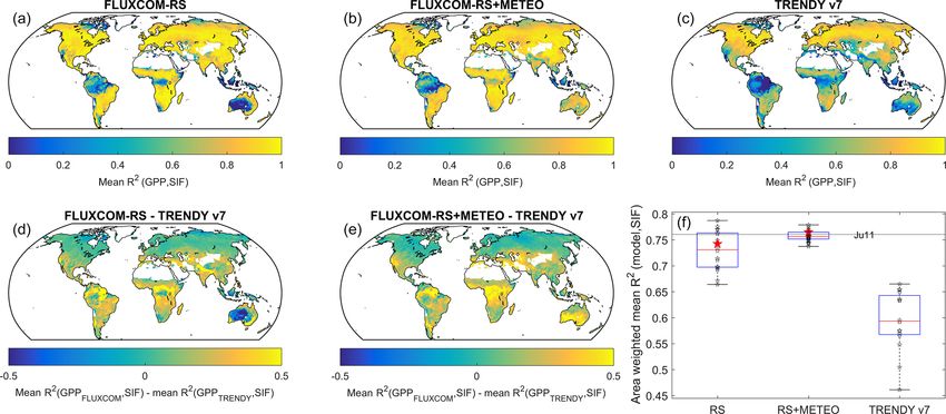
M. Jung et al.: Synthesis and evaluation of the FLUXCOM approach                                                            1347

comparisons to the previous GPP and NEE upscaling prod-          spatial changes. The unstable orbit of the MetOp-A satel-
ucts of Jung et al., 2011 (hereafter referred to as Ju11).       lite that carries one of the GOME-2 instruments and sen-
                                                                 sor degradation effects do not permit conclusive comparisons
2.4     Comparison approach                                      with respect to interannual variability (Zhang et al., 2018).
                                                                 Therefore, we restricted the analysis to mean seasonal cycles
2.4.1    General considerations                                  and show 1◦ maps of the R 2 between mean monthly GPP and
                                                                 SIF.
All products were harmonized to a common 1◦ spatial                 There are remaining caveats and uncertainties associated
resolution with monthly temporal resolution as a basis of        with the GPP–SIF relationship (see e.g. Porcar-Castell et al.,
all comparisons shown here. Cross-consistency checks for         2014 for an overview). Nevertheless, various studies have
mean annual and mean seasonal variations in GPP and NEE          shown that SIF is currently the best proxy for photosynthe-
are based on the 3-year period 2008–2010. The time pe-           sis that can be remotely sensed directly, in particular at sea-
riod is constrained by the availability of GOME-2 data           sonal timescale, and over regions with strong seasonal cy-
starting in 2008 and the corresponding end year of the           cles. This is supported by strong empirical relationships be-
RS+METEO ensemble with the GSWP3 forcing ending in               tween GPP and SIF across different satellites and retrieval
2010. The NEE interannual variability was initially assessed     methods as well as from EC data, crop inventories and data-
for 2001–2010, which is the common period of the RS              driven GPP methods (Frankenberg et al., 2011; Guanter et
and RS+METEO ensembles while comparisons for longer              al., 2014; Joiner et al., 2018; Sun et al., 2017; Walther et al.,
time periods were also facilitated by using meteorological-      2016). This gives us confidence in using SIF as an indepen-
forcing-specific RS+METEO products that cover longer             dent data stream for photosynthesis to evaluate FLUXCOM
time periods (Table 1).                                          products.
   FLUXCOM-RS and FLUXCOM-RS+METEO products
are evaluated mostly separately. We report estimates for         2.4.3   Rationale of comparing net carbon fluxes with
the respective ensemble product (see Sect. 2.1): the spread              atmospheric inversions
over individual ensemble members for uncertainty and the
mean of the ensemble members; the latter can be different        We compared atmospheric inversion-based net carbon re-
from the ensemble product estimate (see Sect. 2.1). Occa-        lease with FLUXCOM mean NEE at the seasonal scale
sionally, we use the range of estimates from the union of        over the established 11 TRANSCOM regions (see Fig. S1
RS and RS+METEO ensemble members to show the full                in the Supplement for a map) as atmospheric inversions
FLUXCOM uncertainty range across the two setups (labelled        are better constrained over large spatial scales (Peylin et
as “FLUXCOM” only). For the comparison of regional or            al., 2013). The comparison of interannual variability was
global flux values, we used flux densities rather than inte-     conducted at the global scale due to its smaller signal
grated fluxes due to inconsistencies in land–sea masks in dif-   and larger transport uncertainties compared to the sea-
ferent products. A common mask of valid data from the in-        sonal cycle. Due to various inversion uncertainties related
tersection of FLUXCOM, TRENDY and Ju11 was applied               to choices of atmospheric transport model, atmospheric sta-
to all data streams, and a land area-weighted regional or        tion CO2 data, fossil fuel information, prior constraints, driv-
global mean was calculated. Globally integrated GPP was          ing wind fields and inversion strategy, we used three differ-
calculated by scaling the global mean GPP density flux with      ent products: Jena CarboScope (s99oc_v4.3, Rödenbeck et
the global non-barren land area (122.4 million km2 ) derived     al., 2018), CAMSv17r1 (Chevallier et al., 2005, 2019) and
from the MODIS land cover product (Friedl et al., 2010).         CarbonTracker-EU (CTE2018, Peters et al., 2010; van der
All reported R 2 values are squared Pearson’s correlation co-    Laan-Luijkx et al., 2017). To evaluate global NEE interan-
efficients, but negative correlation signs are maintained by     nual variability patterns for periods since the late 1950s until
multiplying R 2 values by −1. We aimed at structuring the        present, we further use two long-term atmospheric inversions
cross-consistency checks with SIF and inversion data to min-     (CarboScope s57Xoc_v4.3, sEXTocNEET_v4.3; Rödenbeck
imize confounding factors and uncertainties of the indepen-      et al., 2018) and annual CO2 growth rate from the Global
dent data that may have affected the conclusions otherwise.      Carbon Budget (Le Quéré et al., 2018).
                                                                    It is important to note that FLUXCOM NEE is seman-
2.4.2    Rationale of GPP–SIF comparison                         tically different from inversion-based net carbon exchange
                                                                 between land and atmosphere. The former is solely the
As the GPP–SIF relationship is approximately linear over         difference between gross fluxes (i.e. NEE = TER − GPP)
seasonal timescales (Zhang et al., 2016), the comparison was     while the latter integrates all vertical movement of CO2
based on monthly values. To minimize confounding effects         including, for example, fire emissions, evasion from in-
of canopy structure (e.g. Migliavacca et al., 2017), the com-    land waters, respired harvests or volatile organic compounds
parisons were done over time when canopy structure changes       (Kirschbaum et al., 2019; Zscheischler et al., 2017). Sim-
relative to GPP changes are expected to be much weaker than      ulations from TRENDY models report both NEE and net

www.biogeosciences.net/17/1343/2020/                                                    Biogeosciences, 17, 1343–1365, 2020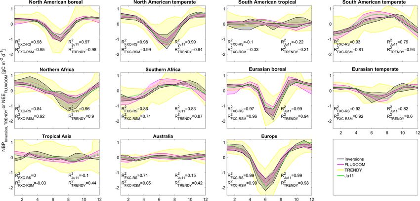
1348                                                     M. Jung et al.: Synthesis and evaluation of the FLUXCOM approach

Figure 2. Comparisons of mean annual GPP at 1◦ spatial resolution for the period 2008–2010 of FLUXCOM ensemble products with Ju11
and the mean of 16 TRENDY models. The diagonal denotes maps of mean annual GPP. Above the diagonal denotes maps of GPP differences
(product along column – product along row). Below the diagonal denotes the 1 : 1 regression where the shading shows point density. The red
line and equations show the best-fit line from total least-squares regression.

biome productivity (NBP), which is conceptually close but              3     Results and discussion
not identical to what atmospheric inversions provide. To
assess whether conclusions are affected by the different               3.1     Gross primary productivity
NEE vs. NBP definitions, we (a) provide NEE and NBP
estimates from TRENDY models, (b) include comparisons                  3.1.1    Mean annual gross primary productivity
where inversions were corrected for fire emissions (from
                                                                       Overall, our results suggest a high degree of cross-product
CarbonTracker-EU) to yield estimates closer to NEE, and
                                                                       (and, for FLUXCOM, also within-product) consistency of
(c) discuss whether discrepancies with FLUXCOM can orig-
                                                                       global mean GPP patterns (Fig. 2). In fact, global patterns
inate from the omission of secondary carbon loss pathways
                                                                       of mean GPP are consistent across both FLUXCOM ensem-
given in the literature.
                                                                       bles (R 2 = 0.97) as well as for Ju11 and TRENDY ensem-
                                                                       ble mean (R 2 > 0.94), despite sizable regional differences.
                                                                       The slope of the pair-wise 1 : 1 regressions among the differ-
                                                                       ent mean GPP data sets varies within ∼ 10 %. FLUXCOM-
                                                                       RS shows about 10 %–20 % lower GPP than FLUXCOM-
                                                                       RS+METEO in the highly productive tropics and some sub-
                                                                       tropical regions. Both FLUXCOM setups estimate larger
                                                                       GPP than Ju11 and TRENDY in some semi-arid regions and
                                                                       about 5 %–15 % lower GPP in some extratropical areas. De-

Biogeosciences, 17, 1343–1365, 2020                                                          www.biogeosciences.net/17/1343/2020/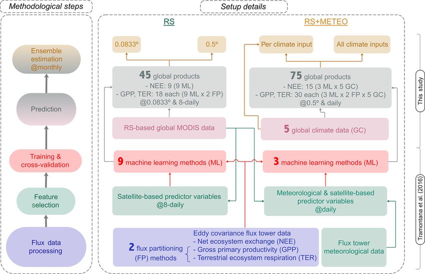
M. Jung et al.: Synthesis and evaluation of the FLUXCOM approach                                                           1349

                                                                  marily due to differences among machine learning methods
                                                                  rather than meteorological forcing data (Fig. S2).
                                                                     Our results imply that the present FLUXNET upscaling
                                                                  approach does not agree with larger GPP values of 150–
                                                                  175 PgC yr−1 derived from an isotope-based study (Welp et
                                                                  al., 2011). It is possible that the FLUXNET upscaling ap-
                                                                  proach underestimates GPP of highly managed and fertil-
                                                                  ized crops (Guanter et al., 2014) but their effects on global
                                                                  GPP biases seem small (Joiner et al., 2018). At FLUXNET
                                                                  sites night-time CO2 advection and storage could cause un-
                                                                  derestimation of night-time CO2 fluxes (Aubinet et al., 2012;
                                                                  McHugh et al., 2017; van Gorsel et al., 2009) and thus un-
                                                                  derestimate GPP using the night-time NEE flux partition-
                                                                  ing method. On the contrary, it has been suggested that
                                                                  FLUXNET GPP estimated from the night-time partitioning
                                                                  method (Reichstein et al., 2005) is overestimated as it ignores
                                                                  the effects of light inhibition of leaf respiration (Keenan
                                                                  et al., 2019; Wehr et al., 2016) by on average 7 % across
                                                                  FLUXNET sites (Keenan et al., 2019). But it should be noted
                                                                  that this value may not be globally representative due to
                                                                  sizable variations between ecosystems and leaf area. Fur-
                                                                  ther, we only find a small difference of mean global GPP
                                                                  of < 2 PgC for daytime (Lasslop et al., 2010) and night-time
                                                                  (Reichstein et al., 2005) NEE partitioning. This suggests that
Figure 3. Map of the fraction of TRENDY models (n = 16) with
                                                                  neither CO2 advection nor the light inhibition of leaf respi-
mean GPP outside the range of FLUXCOM estimates. The FLUX-
COM range is calculated as the maximum minus minimum of all 48    ration appears to generate sizable biases of global GPP in
FLUXCOM members from the union of the RS and RS+METEO             FLUXCOM – a tendency likely encouraged by the relatively
members. Mean GPP was calculated for the period 2008–2010.        strict quality control on the EC flux data (Tramontana et al.,
                                                                  2016). Furthermore, a comparison of EC-based GPP with
                                                                  biometric GPP estimates across 18 globally distributed sites
                                                                  showed good agreement and no significant bias (Campioli et
spite a sizable total range of mean GPP from all 48 FLUX-         al., 2016). A recent study using partitioning based on car-
COM members, the majority of TRENDY models (at least 9            bonyl sulfide (COS) for four contrasting European sites also
out of 16) fall outside the FLUXCOM range for about 70 %          showed good agreement with standard EC-based GPP where
of the land surface (Fig. 3).                                     systematic differences for mean GPP were < 5 % (Spiel-
   The mean global GPP of FLUXCOM-RS (111 PgC yr−1 )              mann et al., 2019). Therefore, we currently have no strong
is about 10 % lower than that of RS+METEO (120 PgC yr−1 ,         indication that systematic biases of FLUXNET GPP prop-
Fig. 4), which is largely driven by differences in the tropics    agate to global FLUXCOM GPP. Nevertheless, we need to
(Fig. 2). The cross-validation analysis indicated an underes-     acknowledge that global GPP is largely driven by the pro-
timation of FLUXCOM-RS GPP in the tropics (Tramontana             ductivity in the tropics where flux towers are scarce and may
et al., 2016), which was confirmed by a grid cell-to-site data    be particularly uncertain due to challenging logistic and mi-
comparison for the FLUXNET 2015 data (which were not              crometeorological conditions (Fu et al., 2018).
used for machine learning training here) (Joiner et al., 2018).      Various remote-sensing-based light use efficiency ap-
The reasons for the on-average lower GPP of RS compared to        proaches, calibrated with flux tower data, yielded global GPP
RS+METEO require further investigation. It is unlikely that       estimates of 109 (Zhao et al., 2005), 111 ± 21 (Yuan et al.,
the RS GPP values are smaller because this setup is exclu-        2010), 108–119 (Yu et al., 2018), 122 ± 25 (Jiang and Ryu,
sively based on remote sensing, as global latent heat from RS     2016), 132±22 (Chen et al., 2012) and 140 PgC yr−1 (Joiner
was larger than Ju11 (Jung et al., 2019). It seems to be rather   et al., 2018). A simple calibration of only near-infrared re-
related to the specifically different predictor sets between RS   flectance (NIRv) to EC data suggested a global GPP of 131–
and RS+METEO. This indicates that future FLUXCOM ef-              163 PgC yr−1 (Badgley et al., 2019). Studies that assimilated
forts should expand the ensemble with respect to predictor        atmospheric CO2 concentration data into process model sim-
set diversity to better account for this source of uncertainty    ulations yielded slightly higher values of 148 (Anav et al.,
in upscaling. Focussing on FLUXCOM-RS+METEO, its en-              2015) and 146 ± 19 PgC yr−1 (Koffi et al., 2012) with the
semble spread (108–130 PgC yr−1 ) is much smaller than the        latter study unable to distinguish their best estimate from a
TRENDY-based global GPPs (83–172 PgC yr−1 ) and is pri-           global GPP of 117 PgC yr−1 because the atmospheric CO2

www.biogeosciences.net/17/1343/2020/                                                     Biogeosciences, 17, 1343–1365, 2020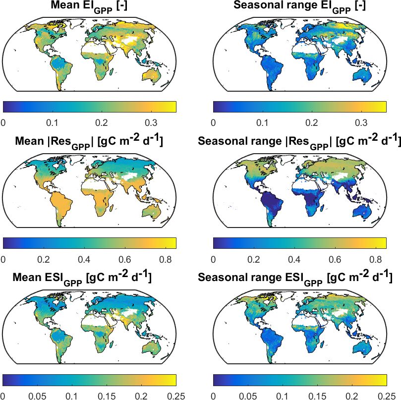
1350                                                      M. Jung et al.: Synthesis and evaluation of the FLUXCOM approach

                                                                      ble members). With SIF, both FLUXCOM setups show con-
                                                                      sistency similar to that of Ju11. The consistency of FLUX-
                                                                      COM with SIF is much better than with TRENDY models,
                                                                      in particular in tropical and subtropical regions. This im-
                                                                      plies that, despite sporadic spatial coverage of FLUXNET
                                                                      sites and previously identified incomplete capturing of wa-
                                                                      ter stress (Bodesheim et al., 2018; Tramontana et al., 2016),
                                                                      FLUXCOM still has a large potential to inform and constrain
                                                                      process-based model simulations of seasonal variations in
                                                                      photosynthesis in moisture-limited regions.

                                                                      3.2     Net ecosystem exchange

                                                                      3.2.1    Mean annual net ecosystem exchange
Figure 4. Global GPP for FLUXCOM and TRENDY ensembles for
the period 2008–2010. The box plots show the median (red line), in-   In most TRANSCOM regions, FLUXCOM shows a stronger
terquartile range (box) and total range (whiskers) of non-outliers    mean annual net carbon uptake than indicated by atmo-
(within median ±1.5 interquartile range) of individual ensemble       spheric inversions with a particularly large systematic dif-
members (open black stars). The filled red star presents the value    ference in the tropics (Fig. 6). This pattern of a large tropical
of the ensemble product (not available for TRENDY). The estimate      carbon sink in FLUXCOM is qualitatively consistent among
of Ju11 is plotted as the horizontal broken line.                     the different FLUXCOM setups and ensemble members, as
                                                                      well as with previous estimates from Ju11. To date, this is
                                                                      a systematic feature of the current data-driven approach of
alone cannot constrain magnitudes of gross fluxes well. As-           upscaling EC measurements with machine learning.
similating SIF into process models yielded 137 ± 6 (Nor-                 Multiple independent approaches indeed imply a sizable
ton et al., 2019) and 166 ± 10 PgC yr−1 (MacBean et al.,              carbon sink in intact tropical forests (Arneth et al., 2017;
2018). More recent isotope studies derived global GPP as              Gaubert et al., 2019; Pan et al., 2011), which appears to be
120 ± 30 PgC yr−1 (Liang et al., 2017) and global net pri-            largely or entirely offset by carbon loss pathways in the trop-
mary productivity (NPP) as ∼ 60 PgC yr−1 (Hellevang and               ical region such as fire, land use change emissions and eva-
Aagaard, 2015), which implies global GPP of 109–150 PgC               sion from inland waters. These CO2 sources are not sampled
yr−1 considering a range of NPP : GPP ratios of 0.4–0.55. In          by EC measurements from FLUXNET and are, therefore,
conclusion, global FLUXCOM GPP estimates are within the               not represented in FLUXCOM. However, the missing fluxes
currently most plausible 110–150 PgC yr−1 range.                      only resolve up to roughly half of the gap (Zscheischler et
                                                                      al., 2017). The comparatively small differences between net
3.1.2   Seasonal cycles of gross primary productivity                 carbon release estimates by inversions and those where fire
                                                                      emissions were corrected for, as well as the small differ-
Cross-consistency analysis of mean monthly GPP seasonal               ences between NEE and NBP from TRENDY, further sug-
cycles from FLUXCOM with SIF from GOME-2 (Köhler                      gest that these secondary carbon loss fluxes do not drive the
et al., 2015) shows widespread and strong agreement for               large discrepancy between FLUXCOM and inversion-based
both FLUXCOM setups (Fig. 5), except for the inner trop-              mean net carbon exchange. Nevertheless, substantial uncer-
ics where seasonality is weak and SIF retrievals might be             tainty remains in the magnitude of these secondary carbon
affected by the South Atlantic Magnetic Anomaly (Köhler et            fluxes and their incomplete accounting in TRENDY models
al., 2015). FLUXCOM-RS tends to show better agreement                 and inversions (Kirschbaum et al., 2019; Zscheischler et al.,
with SIF than FLUXCOM-RS+METEO in agricultural re-                    2017).
gions of Southeast Asia, maybe because only the mean sea-                Issues with the current FLUXCOM approach certainly
sonal cycles of remotely sensed land surface properties were          contribute, and likely dominate, the discrepancy between at-
used in the latter. Conversely, FLUXCOM RS+METEO                      mospheric top-down and FLUXCOM mean NEE. Potential
shows on average better consistency with SIF in some semi-            factors that could contribute to this are (1) a FLUXNET sam-
arid regions, e.g. Australia. However, maps of the maxi-              pling bias (see also Sect. 4.1.2) towards ecosystems with
mum R 2 with SIF for RS and RS+METEO have similar                     a large carbon sink, particularly in the tropics (Saleska et
patterns with good agreement of both products in Australia,           al., 2003), combined with (2) missing predictor variables
and even in the tropics (Fig. S4). This suggests that the in-         related to disturbance and site history (Amiro et al., 2010;
clusion of some machine learning methods somewhat nega-               Besnard et al., 2018; see also Sect. 4.2.1), or (3) biases of
tively impacts the ensemble, especially for RS, which shows           eddy covariance NEE measurements, e.g. due to night-time
larger spread (see Fig. S4 for mean R 2 of the RS ensem-              advection of CO2 (Hayek et al., 2018; van Gorsel et al.,

Biogeosciences, 17, 1343–1365, 2020                                                        www.biogeosciences.net/17/1343/2020/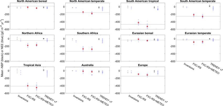
M. Jung et al.: Synthesis and evaluation of the FLUXCOM approach                                                                       1351

Figure 5. Consistency of seasonal GPP variations from FLUXCOM and TRENDY with SIF from GOME-2. Maps in (a, b, c) show the mean
R 2 between mean seasonal cycles for the period 2008–2010, averaged across all respective ensemble members. Difference maps in (d, e, f)
emphasize where FLUXCOM shows better (positive value) and worse (negative value) consistency with SIF than TRENDY and are based
on the maps in the top row. The spatially averaged R 2 values for the different ensembles are summarized in (f). The box plots show the
distribution of individual ensemble members (open black stars). The filled red star presents the value of the ensemble product (not available
for TRENDY). The estimate of Ju11 is plotted as a horizontal line.

2008), especially under tall tropical forest canopies (Hutyra            ally relevant in tropical and subtropical regions. However,
et al., 2008; Fu et al., 2018). Fu et al. (2018) studied 63              adjusting inversion-based NBP towards NEE by correcting
site years of EC data from 13 tropical forest sites and report           for fire emissions does not improve the correspondence with
a mean between-site NEE of −567 gC m−2 yr−1 showing                      FLUXCOM in tropical and subtropical regions (Fig. S5). In
that the large tropical sink in FLUXCOM is inherited from                tropical regions, the weak seasonality paired with compara-
FLUXNET data. The authors pointed out that for about half                tively large spread among inversions does not allow for ro-
of the sites where measurements of CO2 concentration along               bust conclusions. Overall, the seasonal variations in FLUX-
the vertical profile were available and the storage was con-             COM NEE show potential to constrain the large uncertainty
sidered in the NEE processing, the carbon sink was less than             in TRENDY models and potentially even atmospheric inver-
half (−340 gC m−2 yr−1 ) compared to those without storage               sions at the regional scale, especially considering that their
correction (−832 gC m−2 yr−1 ). However, the small sample                uncertainty range across only three products is still signifi-
size together with the large between-site standard deviation             cant.
of mean NEE (459 gC m−2 yr−1 ) not only makes robust con-
clusions difficult, but also indicates potentially large diversity       3.2.3   Interannual variability of net ecosystem exchange
between tropical ecosystems. Clearly, more tropical EC sites
are needed along with a better account of systematic errors
                                                                         Spatial patterns of the magnitude of the interannual vari-
in EC-based NEE measurements to resolve this issue.
                                                                         ability (IAV) of land carbon sink for the period 2001–2010
                                                                         share some common features among atmospheric inversions,
3.2.2   Seasonal cycles of net ecosystem exchange                        FLUXCOM-RS, FLUXCOM-RS+METEO and TRENDY.
                                                                         For example, all products identify the hotspots in South-
We find a good consistency between FLUXCOM and inver-                    east Asia, southern North America and also the Siberian tun-
sions with respect to amplitude and shape of the seasonal cy-            dra (Fig. 8). Overall, there are still differences in the spatial
cles of NEE in many TRANSCOM regions, especially over                    patterns of IAV magnitude among and within different data
the North American boreal, North American temperate and                  streams.
European regions with R 2 values > 0.92 (Fig. 7). As with                   All EC data-driven methods, in particular FLUXCOM-
mean annual NEE, the seasonal cycle mismatch relative to                 RS+METEO, underestimate magnitude of IAV compared to
inversions may be linked to carbon loss fluxes not accounted             inversions (Fig. 8). The reasons for the underestimation of
for in FLUXCOM, such as fire emissions that are season-                  IAV magnitude by FLUXCOM are not fully clear. Within

www.biogeosciences.net/17/1343/2020/                                                              Biogeosciences, 17, 1343–1365, 2020
1352 M. Jung et al.: Synthesis and evaluation of the FLUXCOM approach Figure 6. Mean annual net carbon release for the years 2008–2010 over TRANSCOM regions. Crosses refer to individual ensemble members where black refers to negative net biome productivity (NBP, not available for FLUXCOM), and blue refers to net ecosystem exchange (NEE). For inversions, NEE was approximated by correcting NBP with fire emissions (see Sect. 2.4.3). The filled red stars refer to estimates by the ensemble product of FLUXCOM setups. The horizontal line indicates the estimate of Ju11. FLUXCOM, the smaller IAV magnitude of RS+METEO 0.31 to 0.60, Fig. S8). This indicates that machine learning NEE compared to that of RS is linked to the use of only methods can benefit from higher temporal variability pro- mean seasonal cycles of RS-based land surface properties in vided by millions of high-frequency NEE measurements, es- the RS+METEO setup. The IAV of carbon loss fluxes that pecially for signals such as IAV that are small and difficult to are not captured by FLUXCOM, such as through fire, is cur- extract. In addition, underlying functional relationships can rently thought to be comparatively small at the global scale be better extracted from high-frequency data as the predictor and appear minor here (see Fig. S6). Machine learning meth- space is better covered, allowing for improved discrimination ods already underestimate the IAV at the site level (Marcolla of drivers that have stronger covariation on longer timescales. et al., 2017; Tramontana et al., 2016). The low bias in FLUX- To better understand the qualitatively different global NEE COM IAV is a direct consequence of the comparatively small IAV patterns between RS and RS+METEO setups, we in- explained variance for NEE anomalies. Thus, improving the fer which NEE IAV signals are consistent or lacking among predictability of NEE IAV at the site level has potential to FLUXCOM setups and TRENDY models by assessing cor- also correct the magnitude of globally integrated IAV vari- relation patterns (Fig. 9). We find the strongest consisten- ance. cies of NEE IAV between FLUXCOM-RS and FLUXCOM- Despite the tendency of FLUXCOM products to under- RS+METEO in many semi-arid regions and almost no con- estimate IAV magnitude, FLUXCOM-RS+METEO repro- sistency otherwise. This suggests that the main discrepan- duces year-to-year variations in globally integrated annual cies of globally integrated NEE IAV between FLUXCOM- land carbon exchange anomalies derived from atmospheric RS and FLUXCOM-RS+METEO are likely not due to dif- inversions for 2001–2010 (R 2 = 0.87). It shows better con- ferences in their capabilities of reflecting water stress ef- sistency than TRENDY with one of the long-term inversions fects. It has been shown that despite the local dominance, (Fig. S7). Further examination of this ensemble reveals that water-related NEE anomalies largely cancel spatially in the choice of machine learning method, rather than meteoro- RS+METEO and TRENDY, resulting in the dominance of logical forcing data, has a larger influence on IAV of global temperature-related NEE anomalies in globally integrated NEE (Fig. S8). Here, the random-forest method performed land sink IAV (Jung et al., 2017, but see Humphrey et al., less well compared to the other two methods. Interestingly, 2018, for a different perspective). Studies on effects of wa- training random forests with an almost identical predictor set ter availability on spatial GPP anomalies using the RS data but at a half-hourly temporal scale rather than at a daily scale yielded highly plausible patterns that were consistent with in- (Bodesheim et al., 2018) substantially improved the R 2 (from dependent data (Flach et al., 2018; Orth et al., 2019; Walther Biogeosciences, 17, 1343–1365, 2020 www.biogeosciences.net/17/1343/2020/
M. Jung et al.: Synthesis and evaluation of the FLUXCOM approach                                                               1353

Figure 7. Mean seasonal variations in net land carbon release for the period 2008–2010 over TRANSCOM regions. For inversions and
TRENDY, NBP was plotted, and for FLUXCOM, NEE was plotted. Please note that the region-specific mean was removed for each data
set. Shading indicates the range of estimates (maximum – minimum). The FLUXCOM range is based on the union of RS and RS+METEO
ensemble members. R 2 values were calculated with the mean of the inversions. The FLUXCOM RS and RS+METEO refer to the ensemble
products (median), while those for TRENDY refer to the model mean.

et al., 2019). Also, the comparison of FLUXCOM-RS GPP              spect to NEE IAV at FLUXNET sites (Tramontana et al.,
monthly anomalies with the independent FLUXNET2015                 2016; Morales et al., 2005). However, both approaches yield
data set showed unexpectedly high consistency when anoma-          good correspondence of globally integrated NEE with atmo-
lies were scaled by the site-specific observational range          spherically derived interannual land sink variations. This cor-
(Joiner et al., 2018). When delineating the regions with larger    respondence is due to two reasons: first, the spatial com-
agreement between RS+METEO and TRENDY than that                    pensation of locally important processes that are not well
between RS and TRENDY, we can infer that FLUXCOM-RS                captured by the models, and, second, models better capture
seems to miss important NEE anomaly features in the tropics.       the temperature-related signals that gain relevance at larger
This is likely due to (1) a combination of sparse satellite data   spatial scales (Jung et al., 2017). Whether the large uncer-
availability, cloud contamination and geometrical illumina-        tainty of modelling NEE IAV at the ecosystem level is due to
tion effects in the tropics or (2) that the processes govern-      misspecified parameterizations, missing predictors, inaccu-
ing NEE IAV in the tropics cannot be captured by satellite-        rate forcing data and/or absent processes remains a research
based predictors alone in RS (even under ideal observational       priority. Our understanding and ability to model NEE IAV
conditions) but require additional meteorological variables        bottom-up would greatly benefit from atmospheric inver-
such as temperature that are included in the RS+METEO              sions that could localize NEE robustly. Exploiting the mas-
setup. Some support for the latter point comes from Byrne et       sive space-based column CO2 data in the future will hope-
al. (2019), who found strong correlations of anomalies from        fully facilitate improvements on this aspect. Despite large
GOSAT inversions with NEE from RS+METEO and soil                   uncertainties and apparent knowledge gaps in NEE IAV from
temperatures in the tropics but not with SIF and a drought in-     both an observational and modelling perspective, there are
dicator, suggesting that temperature impacts respiration more      promising indications of improved capability to track IAV
than photosynthesis in the tropics.                                patterns with FLUXCOM such as the good correspondence
   Overall there are large discrepancies between FLUXCOM           of RS+METEO with inversions at the global scale and inde-
and TRENDY as well as amongst TRENDY models with re-               pendent verifications of GPP IAV of RS at least outside the
spect to local NEE IAV. This reflects our limited understand-      wet tropics (Flach et al., 2018; Joiner et al., 2018; Orth et al.,
ing and capabilities to model year-to-year variations in local     2019; Walther et al., 2019).
ecosystem carbon exchange. Both data-driven and process-
based approaches also showed poor performance with re-

www.biogeosciences.net/17/1343/2020/                                                       Biogeosciences, 17, 1343–1365, 2020
1354 M. Jung et al.: Synthesis and evaluation of the FLUXCOM approach
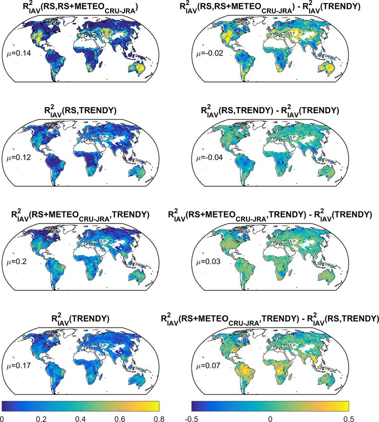
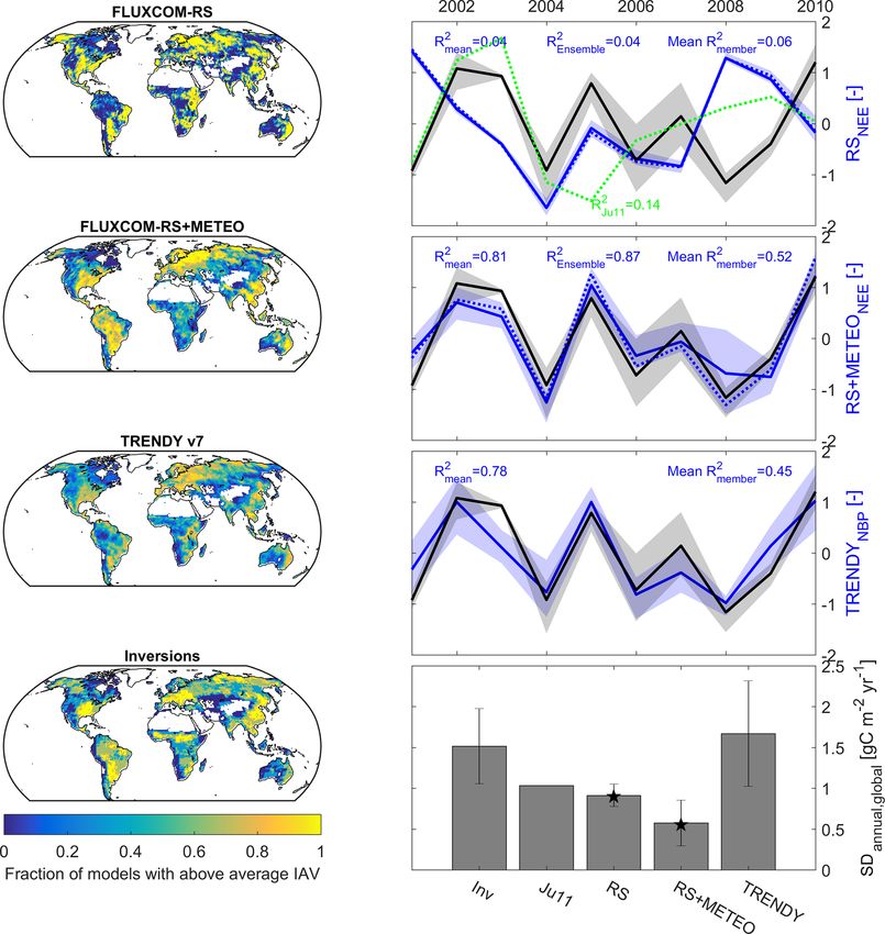
Figure 8. Interannual variability patterns of FLUXCOM NEE, TRENDY NBP and NBP from three atmospheric inversions for the period
2001–2010. Maps show the fraction of respective ensemble members with above-average interannual variability (standard deviation of annual
values multiplied with land area). Time series plots show detrended globally integrated annual NEE or NBP anomalies normalized by their
standard deviation. The black line is the mean of three inversions and the grey shading indicates their range. The blue solid lines are the
means of the considered ensembles; the blue dashed lines are the FLUXCOM ensemble products. R 2 values refer to the comparison with the
mean of inversions (black solid line). The bar chart in the bottom right panel shows the standard deviation of detrended annual NEE or NBP
for different data sets, averaged over the ensemble members, and the error bar indicates the standard deviation of the ensemble members.
Black stars for FLUXCOM refer to the value for the ensemble products.
4 Methodological limitations and potential ways opment of machine learning notwithstanding, we believe that
forward the FLUXCOM approach is at present more limited by avail-
able “information” rather than by available machine learning
methods.
Machine learning methods can learn arbitrarily complex
functions and provide a nearly perfect model of a phe- 4.1 FLUXNET observations
nomenon if they are fed with the right data and trained thor-
oughly. Thus the quality, quantity and completeness of the 4.1.1 Potential observation errors
input data determine the quality of the output. In the follow-
ing, we discuss the relevance of limitations associated with The comparatively large random errors of high-frequency EC
data from the FLUXNET network and of the limited capa- measurements diminish quickly when aggregated to daily or
bilities of representing all relevant factors by observable pre- 8 d averages used here. Furthermore, training on half-hourly
dictor variables. We also outline potential strategies for im- EC data (Bodesheim et al., 2018) helps machine learning
provements, both overall and with respect to machine learn- methods extract patterns from noisy data. In general, poor
ing approaches specifically. The continued and rapid devel- signal-to-noise ratios can be counteracted by larger sam-
Biogeosciences, 17, 1343–1365, 2020 www.biogeosciences.net/17/1343/2020/M. Jung et al.: Synthesis and evaluation of the FLUXCOM approach 1355 Figure 9. Consistency between interannual variabilities (IAV) of local NEE from FLUXCOM setups and TRENDY for the period 2001– 2015. ple size. More problematic than random errors are poten- all these issues together seem to be relatively small compared tial systematic errors of EC measurements since those would to the predominant patterns of variability in EC data, e.g. sea- propagate to the derived global carbon flux products. Even sonal variations, that are very consistent across FLUXCOM though there have been large efforts by the community to and independent observation-based data streams shown here. characterize and to correct for systematic errors, such as The relatively strict quality controls on the flux training data those due to low turbulence and CO2 advection (e.g. Aubi- (Tramontana et al., 2016) may have been instrumental here. net et al., 2005, 2012; Papale et al., 2006), uncertainties re- The trade-off between data quality and training data volume main on the relevance and magnitude of those errors in the was not explicitly studied in FLUXCOM, and related exper- processed FLUXNET data. Differences due to instrumenta- imental setups would be desirable to gauge the robustness tion and maintenance pose another potential source of un- of the global products shown here. Even small systematic certainty. Additionally, the energy balance closure gap at errors in EC data could degrade important signals such as FLUXNET sites is still not resolved (Stoy et al., 2013), while interannual variability, trends, annual sums of NEE or sub- it remains unclear to what extent this is relevant for CO2 tle differences between sites related to functional properties fluxes (Leuning et al., 2012). Systematic errors in GPP and (e.g. radiation use efficiency). Systematic errors that would TER derived from the flux partitioning method of NEE based be prevalent across the network would result in systematic on night-time data (Reichstein et al., 2005) may arise due to biases of derived global fluxes. For global GPP and energy the neglected effect of inhibited photorespiration during day- fluxes (Jung et al., 2019), the values obtained from FLUX- time (Keenan et al., 2019; Wehr et al., 2016). Nevertheless, COM are generally consistent with current knowledge but www.biogeosciences.net/17/1343/2020/ Biogeosciences, 17, 1343–1365, 2020
1356                                                      M. Jung et al.: Synthesis and evaluation of the FLUXCOM approach

Figure 10. Mean annual (2001–2015) and seasonal range (8 d time step) of the extrapolation index (EI), the expected mean absolute error of
machine learning predictions, and the extrapolation severity index (ESI, product of the previous two) (see Fig. S2 for details) for GPP from
FLUXCOM-RS.

our ability to independently quantify such fluxes is also lim-          dictor variables. This might be challenging, especially for
ited.                                                                   remote sensing products, due to necessary but complicated
                                                                        corrections of illumination conditions. The uncertainties of
4.1.2   Potential representation issues                                 these topographic factors might become particularly relevant
                                                                        and should be studied for prediction of fluxes at a higher
                                                                        spatial resolution. For the current FLUXCOM products with
Ideally, a measurement network samples all relevant gradi-
                                                                        rather coarse spatial resolution, we expect that topographic
ents of the driving factors and magnitudes of the predicted
                                                                        effects are reflected in the predictor variables and the remain-
quantities. There are several potential issues with the cur-
                                                                        ing subpixel heterogeneity largely cancels out.
rent sampling by FLUXNET sites. With respect to relevance
                                                                           Perhaps the most fundamental and frequent critique of
for net carbon exchange, there are carbon loss pathways that
                                                                        the FLUXNET upscaling approach is related to the spatially
FLUXNET does not capture such as fire emissions, CO2 eva-
                                                                        clumped geographic distribution of EC sites in North Amer-
sion from inland waters, and lateral exports due to harvest or
                                                                        ica, Europe, Japan and now Australia with only sparsely dis-
erosion that are respired elsewhere (Kirschbaum et al., 2019).
                                                                        tributed towers elsewhere (Schimel et al., 2015). However,
The effects of strongly enhanced respiration in the years af-
                                                                        what matters eventually for machine learning methods is how
ter large disturbances (Amiro et al., 2010) are challenging to
                                                                        well the predictor space, rather than geographic space, is
capture due to the stochastic and destructive nature of distur-
                                                                        sampled. To assess this, we developed an extrapolation in-
bances.
                                                                        dex (EI) that estimates the expected additional relative er-
   To meet the assumptions of the EC method, FLUXNET
                                                                        ror of a flux prediction due to a large distance to the nearest
stations are confined to reasonably flat terrain. Topographic
                                                                        training datum in the predictor space (S2). We applied this
effects on ecosystem fluxes are primarily due to their influ-
                                                                        method for GPP and FLUXCOM-RS training data as an ex-
ence on environmental drivers, i.e. the predictor variables.
                                                                        ample, and we found that the conditions that are least well
Thus, the extrapolation to hillslopes should be reasonable if
                                                                        represented by FLUXNET are associated with primarily ex-
the topographic effects are accounted for in the gridded pre-

Biogeosciences, 17, 1343–1365, 2020                                                           www.biogeosciences.net/17/1343/2020/
M. Jung et al.: Synthesis and evaluation of the FLUXCOM approach 1357
tremely cold and dry regions (Fig. 10). Surprisingly, the hu- 4.2 Driving factors and predictors
mid tropics are well represented in the predictor space, sug-
gesting that the environmental conditions represented by the Assuming infinite sample size and perfect quality and cov-
predictor set are well sampled by the data from FLUXNET erage, the success of machine learning methods depends en-
sites. The extremely cold and dry conditions that seem to tirely on the completeness of the predictor set for the tar-
constitute the biggest extrapolation issues are typically asso- get variable, given an adequate training. The predictor set
ciated with small GPP fluxes and thus also small prediction for FLUXNET upscaling is practically constrained by (1) the
errors. To account for that, we spatialized the expected GPP availability of consistent observations at the site level across
error of the RS ensemble (Figs. 10, S2 for details), which all sites, and for most of their temporal coverage at a spa-
largely scales with GPP magnitude but also shows patterns tial resolution sufficiently close to the flux tower footprint,
of larger expected errors in semi-arid regions than those ex- and (2) the availability of corresponding global grids at an
pected from flux magnitude alone. The multiplication of the adequate spatial and temporal resolution and temporal cov-
expected GPP error with the extrapolation index provides erage. This explains the predictor space of remotely sensed
the extrapolation severity index (ESI) that shows where poor land products from MODIS along with tower-measured me-
FLUXNET sampling likely increases the absolute prediction teorology chosen in FLUXCOM. While the general success
error strongly. According to these results, subtropical semi- of the FLUXCOM approach suggests that the predictor sets
arid regions, in particular India, appear most affected, sug- contain sufficient information for predicting the variability of
gesting that GPP upscaling from FLUXNET would benefit carbon fluxes, it is also obvious that some factors are not well
most strongly from improved data availability for towers rep- accounted for.
resenting these conditions. Despite these limitations of data,
we found excellent consistency of FLUXCOM GPP seasonal
cycles with SIF over these regions, which was in fact much 4.2.1 Site history
better than the consistency between TRENDY models and
SIF. This suggests that while more towers in semi-arid re- It has been argued previously (Besnard et al., 2018; Jung et
gions will help reduce uncertainty in future upscaling efforts, al., 2011; Tramontana et al., 2016) that the current limitations
FLUXCOM can already provide useful information for con- of unrealistic mean NEE patterns from FLUXNET upscaling
straining the models in these regions. It also shows that the are also due to missing predictor variables that describe site
bias in geographic representation of FLUXNET sites is not history effects such as forest age or time since disturbance.
as critical as anticipated due to the flexibility and adaptive- These factors have been shown to influence IAV (Musavi et
ness of machine learning methods. The sampled environmen- al., 2017; Tamrakar et al., 2018) and to drive mean NEE pat-
tal conditions (predictor space) should cover the conditions terns in synthesis studies (e.g. Amiro et al., 2010). Including
of the global application domain rather than being represen- forest age in a simple empirical model helped predict be-
tative of it. The larger issue of the FLUXNET representation tween site variations in mean NEE across FLUXNET sites
bias is associated with drawing conclusions from the site- (Besnard et al., 2018). Counterintuitively, including forest
level cross-validation because the evaluation metrics are eas- age in training a machine learning method on monthly NEE
ily biased towards certain regions and ecosystems. did not improve the predictability of mean site NEE (Besnard
The methodology used here to assess the extrapolation et al., 2019), albeit possibly due to data or methodological
problem quantitatively has several limitations. For example, limitations. We find the largest discrepancies of mean FLUX-
potential differences in EC data quality were not accounted COM NEE with atmospheric inversions in the tropics, where
for. Perhaps the largest but unavoidable limitation is the re- site history plays a substantial role in NEE magnitude (Pugh
liance on the predictor set and the assumption that it cap- et al., 2019), but the concept of forest age is hardly appli-
tures all relevant gradients. In a sense, the methodology can cable due to the generally uneven aged nature of stands, and
only uncover “known unknowns”. If an important predictor reliable estimates of gridded age, e.g. from forest inventories,
is missing, the method would, of course, not see any extrap- are not available. Efforts to incorporate the information from
olation penalty with respect to the missing factor. Somewhat long-term Landsat time series to capture site history effects
ironically, we may need more towers in the first place to iden- did not reveal an improvement in the predictions of mean
tify further relevant predictors in an objective way to, say, NEE, but it remains unclear if this was due to limited infor-
better capture the diversity in the tropics (Fu et al., 2018) or mation content in these time series or due to methodological
in agricultural systems (Guanter et al., 2014) where we an- issues (Besnard et al., 2019). Thus, this issue remains a sig-
ticipate that the current sampling is limiting the FLUXCOM nificant scientific challenge. Potentially, the availability and
approach. application of high-resolution biomass and vegetation optical
depth estimates from radar remote sensing along with care-
fully collected ancillary data on biomass, basal area, tree di-
ameter and tree age distributions at ICOS and NEON sites
may help in the future.
www.biogeosciences.net/17/1343/2020/ Biogeosciences, 17, 1343–1365, 2020You can also read