Measuring Congestion in High-Performance Datacenter Interconnects - USENIX
←
→
Page content transcription
If your browser does not render page correctly, please read the page content below

Measuring Congestion in High-Performance
         Datacenter Interconnects
   Saurabh Jha and Archit Patke, University of Illinois at Urbana-Champaign; Jim
 Brandt and Ann Gentile, Sandia National Lab; Benjamin Lim, University of Illinois
  at Urbana-Champaign; Mike Showerman and Greg Bauer, National Center for
    Supercomputing Applications; Larry Kaplan, Cray Inc.; Zbigniew Kalbarczyk,
University of Illinois at Urbana-Champaign; William Kramer, University of Illinois at
Urbana-Champaign and National Center for Supercomputing Applications; Ravi Iyer,
                       University of Illinois at Urbana-Champaign
               https://www.usenix.org/conference/nsdi20/presentation/jha

        This paper is included in the Proceedings of the
    17th USENIX Symposium on Networked Systems Design
                and Implementation (NSDI ’20)
                   February 25–27, 2020 • Santa Clara, CA, USA
                                  978-1-939133-13-7

                                          Open access to the Proceedings of the
                                         17th USENIX Symposium on Networked
                                          Systems Design and Implementation
                                               (NSDI ’20) is sponsored by
Measuring Congestion in High-Performance Datacenter Interconnects

                Saurabh Jha1 , Archit Patke1 , Jim Brandt2 , Ann Gentile2 , Benjamin Lim1 ,
    Mike Showerman3 , Greg Bauer3 , Larry Kaplan4 , Zbigniew Kalbarczyk1 , William Kramer1,3 , Ravi Iyer1
                      1 University   of Illinois at Urbana-Champaign, 2 Sandia National Lab,
                          3 National  Center for Supercomputing Applications, 4 Cray Inc.

                         Abstract                                 analysis which may be difficult to perform at runtime.
While it is widely acknowledged that network congestion              The core contributions of this paper are (a) a methodol-
in High Performance Computing (HPC) systems can signifi-          ogy, including algorithms, for quantitative characterization
cantly degrade application performance, there has been little     of congestion of high-speed interconnect networks; (b) in-
to no quantification of congestion on credit-based intercon-      troduction of a deployable toolset, Monet [7], that employs
nect networks. We present a methodology for detecting, ex-        our congestion characterization methodology; and (c) use of
tracting, and characterizing regions of congestion in networks.   the the methodology for characterization of congestion using
We have implemented the methodology in a deployable tool,         5 months of operational data from a 3D torus-based inter-
Monet, which can provide such analysis and feedback at run-       connect network of Blue Waters [1, 27, 60], a 13.3-petaflop
time. Using Monet, we characterize and diagnose congestion        Cray supercomputer at the National Center for Supercom-
in the world’s largest 3D torus network of Blue Waters, a 13.3-   puting Applications (NCSA) at the University of Illinois at
petaflop supercomputer at the National Center for Supercom-       Urbana-Champaign. The novelty of our approach is its ability
puting Applications. Our study deepens the understanding of       to use percent time stalled (PT s )1 metric to detect and quan-
production congestion at a scale that has never been evaluated    titatively characterize congestion hotspots, also referred to
before.                                                           as congestion regions (CRs), which are group of links with
                                                                  similar levels of congestion.
1     Introduction                                                   The Monet tool has been experimentally used on NCSA’s
   High-speed interconnect networks (HSN), e.g., Infini-          Blue Waters. Blue Waters uses a Cray Gemini [21] 3D torus
band [48] and Cray Aries [42]), which uses credit-based flow      interconnect, the largest known 3D torus in existence, that
control algorithms [32, 61], are increasingly being used in       connects 27,648 compute nodes, henceforth referred to as
high-performance datacenters (HPC [11] and clouds [5, 6, 8,       nodes. The proposed tool is not specific to Cray Gemini and
80]) to support the low-latency communication primitives          Blue Waters; it can be deployed on other k-dimensional mesh
required by extreme-scale applications (e.g., scientific and      or toroidal networks, such as TPU clouds [3], Fujitsu TOFU
deep-learning applications). Despite the network support for      network-based [18, 20] K supercomputer [70] and upcoming
low-latency communication primitives and advanced conges-         post-K supercomputer [10]2 . The key components of our
tion mitigation and protection mechanisms, significant perfor-    methodology and the Monet toolset are as follows:
mance variation has been observed in production systems run-         Data collection tools: On Blue Waters, we use vendor-
ning real-world workloads. While it is widely acknowledged        provided tools (e.g., gpcdr [35]), along with the Lightweight
that network congestion can significantly degrade application     Distributed Metric Service (LDMS) monitoring frame-
performance [24, 26, 45, 71, 81], there has been little to no     work [17]. Together these tools collect data on (a) the network
quantification of congestion on such interconnect networks        (e.g., transferred/received bytes, congestion metrics, and link
to understand, diagnose and mitigate congestion problems          failure events); (b) the file system traffic (e.g., read/write
at the application or system-level. In particular, tools and      bytes); and (c) the applications (e.g., start/end time). We are
techniques to perform runtime measurement and characteri-         released raw network data obtained from Blue Waters [57] as
zation and provide runtime feedback to system software (e.g.,     well as the associated code for generating CRs as artifacts with
schedulers) or users (e.g., application developers or system      this paper [7]. To the best of our knowledge, this is the first
managers) are generally not available on production systems.      1P ,   defined formally in Section 2, approximately represents the intensity
                                                                    Ts
This would require continuous system-wide, data collection          of congestion on a link, quantified between 0% and 100%.
on the state of network performance and associated complex        2 The first post-K supercomputer is scheduled to be deployed in 2021.

USENIX Association                           17th USENIX Symposium on Networked Systems Design and Implementation                         37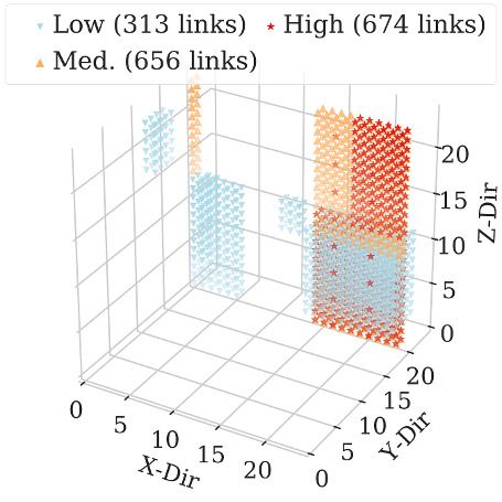
directionally
Congestion Region 8 links maps Z+ Z-
§2 System §3 Data Collection §4 (CR) extraction using
Use cases to 8 tiles 8 8
aggregated
Description CR DB links
Scheduler unsupervised clustering Congestion
2 MB X+ 8 4 Y+
48 tiles
§6 response and
(Moab), 7 GB
Network monitors §5 Characterization mitigation X- 8 }
AAAB6XicbVBNS8NAEJ3Ur1q/qh69LBbBU0m0YI8FLx6r2A9oQ9lsJ+3SzSbsboQS+g+8eFDEq//Im//GbZuDtj4YeLw3w8y8IBFcG9f9dgobm1vbO8Xd0t7+weFR+fikreNUMWyxWMSqG1CNgktsGW4EdhOFNAoEdoLJ7dzvPKHSPJaPZpqgH9GR5CFn1FjpoT8blCtu1V2ArBMvJxXI0RyUv/rDmKURSsME1brnuYnxM6oMZwJnpX6qMaFsQkfYs1TSCLWfLS6dkQurDEkYK1vSkIX6eyKjkdbTKLCdETVjverNxf+8XmrCup9xmaQGJVsuClNBTEzmb5MhV8iMmFpCmeL2VsLGVFFmbDglG4K3+vI6aV9Vveuqd1+rNOp5HEU4g3O4BA9uoAF30IQWMAjhGV7hzZk4L86787FsLTj5zCn8gfP5A5yGjWA=
4 Y-
Gemini ASIC
(Cray xtnlrd), 100 GB
CR size §7 Diagnosing
Blue Waters Performance metrics CR duration causes of 4 4 links
… congestion
(3D Torus) samplers (LDMS), 15 TB CR growth NIC0 NIC1
Figure 1: Characterization and diagnosis workflow for interconnection-networks. Figure 2: Cray Gemini 48-port switch.
such large-scale network data release for an HPC high-speed in the next measurement window.
interconnect network that uses credit-based flow control. • Quick propagation of congestion can be caused by net-
A network hotspot extraction and characterization work component failures. Network component failures
tool, which extracts CRs at runtime; it does so by using an (e.g., network router failures) that occur in the vicinity of a
unsupervised region-growth clustering algorithm. The clus- large-scale application can lead to high network congestion
tering method requires specification of congestion metrics within minutes of the failure event. Measurements show
(e.g., percent time stalled (PT s ) or stall-to-flit ratios) and a that 88% of directional link failures 5 caused the formation
network topology graph to extract regions of congestion that of CRs with an average PT s ≥ 15%.
can be used for runtime or long-term network congestion • Default congestion mitigation mechanisms have limited
characterization. efficacy. Our measurements show that (a) 29.8% of the 261
A diagnosis tool, which determines the cause of conges- triggers of vendor-provided congestion mitigation mecha-
tion (e.g., link failures or excessive file system traffic from nisms failed to alleviate long-lasting congestion (i.e., con-
applications) by combining system and application execution gestion driven by continuous oversubscription, as opposed
information with the CR characterizations. This tool leverages to isolated traffic bursts), as they did not address the root
outlier-detection algorithms combined with domain-driven causes of congestion; and (b) vendor-provided mitigation
knowledge to flag anomalies in the data that can be correlated mechanisms were triggered in 8% (261) of the 3,390 high-
with the occurrence of CRs. congestion events identified by our framework. Of these
To produce the findings discussed in this paper, we used 3,390 events, 25% lasted for more than 30 minutes. This
5 months of operational data on Blue Waters representing analysis suggests that augmentation of the vendor-supplied
more than 815,006 unique application runs that injected more solution could be an effective way to improve overall con-
than 70 PB of data into the network. Our key findings are as gestion management.
follows:
In this paper, we highlight the utility of congestion regions in
• While it is rare for the system to be globally congested,
the following ways:
there is a continuous presence of highly congested regions
(CRs) in the network, and they are severe enough to affect • We showcase the effectiveness of CRs in detecting long-
application performance. Measurements show that (a) for lived congestion. Based on this characterization, we pro-
more than 56% of system uptime, there exists at least one pose that CR detection could be used to trigger congestion
highly congested CR (i.e., a CR with a PT s > 25%), and that mitigation responses that could augment the current vendor-
these CRs have a median size of 32 links and a maximum provided mechanisms.
size of 2,324 links (5.6% of total links); and (b) highly • We illustrate how CRs, in conjunction with network traf-
congested regions may persist for more than 23 hours, with fic assessment, enable congestion diagnosis. Our diagno-
a median duration time of 9 hours3 . With respect to impact sis tool attributes congestion cause to one of the follow-
on applications, we observed 1000-node production runs ing: (a) system issues (such as launch/exit of application),
of the NAMD [77] application 4 slowing down by as much (b) failure issues (such as network link failures), and (c)
as 1.89× in the presence of high congestion compared to intra-application issues (such as changes in communication
median runtime of 282 minutes. patterns within an application). Such a diagnosis allows
• Once congestion occurs in the network, it is likely to persist system managers to take cause-specific mitigating actions.
rather than decrease, leading to long-lived congestion in This paper’s organization is illustrated in Figure 1. We
the network. Measurements show that once the network present background information on the Gemini network, per-
has entered a state of high congestion (PT s > 25%), it will formance data, and congestion mitigation mechanisms in Sec-
persist in high congestion state with a probability of 0.87 tion 2. In Section 3, we present our data collection method-
ology and tools. In Section 4, we present our methodology
3 Note that Blue Waters allows applications to run for a maximum of 48 hours. for characterizing congestion. We present our measurement-
4 NAMD is the top application running on Blue Waters consuming 18% of
total node-hours [58]. 5 see Section 5.4 for the definition of directional link.
38 17th USENIX Symposium on Networked Systems Design and Implementation USENIX Association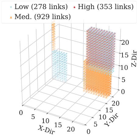
driven congestion characterization results in Section 5. In               hops in + or - chosen for each direction. A deterministic rule
Section 6, we discuss the further utility of our methodology              handles tie-breaking.
to inform targeted responses, and in Section 7, we discuss its               To avoid data loss in the network 7 , the Gemini HSN uses a
use in diagnosing the root causes of congestion. We address               credit-based flow control mechanism [61], and routing is done
related work in Section 8 and conclude in Section 9.                      on a per-packet basis. In credit-based flow control networks,
                                                                          a source is allowed to send a quantum of data, e.g., a flit, to
2     Cray Gemini Network and Blue Waters                                 a next hop destination only if it has a sufficient number of
   A variety of network technologies and topologies have been             credits. If the source does not have sufficient credits, it must
utilized in HPC systems (e.g., [19, 21, 31, 36, 42, 59, 62, 75]).         stall (wait) until enough credits are available. Stalls can occur
Depending on the technology, routing within these networks                in two different places: within the switch (resulting in a inq
may be statically defined for the duration of a system boot cy-           stall) or between switches (resulting in an credit stall).
cle, or may dynamically change because of congestion and/or
failure conditions. More details on HPC interconnects can be              Definition 1 : A Credit stall is the wait time associated with
found in Appendix A. The focus of this paper is on NCSA’s                 sending of a flit from an output buffer of one switch to an input
Cray XE/XK Blue Waters [1] system, which is composed of                   buffer of another across a link.
27,648 nodes and has a large-scale (13,824 x 48 port switches)
Gemini [21] 3D torus (dimension 24x24x24) interconnect. It                Definition 2 : An Inq stall is the wait time associated with
is a good platform for development and validation of conges-              sending of a flit from the output buffer of one switch port to an
tion analysis/ characterization methods as:                               input buffer of another between tiles within the same network
• It uses directional-order routing, which is predominantly               switch ASIC.
   static6 . From a traffic and congestion characterization per-
                                                                          Congestion in a Gemini-based network can be characterized
   spective, statically routed environments are easier to vali-
                                                                          using both credit and inq stall metrics. Specifically, we con-
   date than dynamic and adaptive networks.
                                                                          sider the Percent Time Stalled as a metric for quantifying
• Blue Waters is the best case torus to study since it uses
                                                                          congestion, which we generically refer to as the stall value.
   topology-aware scheduling (TAS) [41, 82], discussed later
   in this section, which has eliminated many congestion is-              Definition 3 : Percent Time Stalled (PT s ) is the average time
   sues compared to random scheduling.                                    spent stalled (Tis ) over all tiles of a directional network link
• Blue Waters performs continuous system-wide collection                  or individual intra-Gemini switch link over the same time
   and storage of network performance counters.                           interval (Ti ): PT s = 100 ∗ Tis /Ti .
2.1      Gemini Network
                                                                             Depending on the network topology and routing rules, (a)
   In Cray XE/XK systems, four nodes are packaged on a                    an application’s traffic can pass through switches not directly
blade. Each blade is equipped with a mezzanine card. This                 associated with its allocated nodes, and multiple applications
card contains a pair of Gemini [21] ASICs, which serve as                 can be in competition for bandwidth on the same network
network switches. The Gemini switch design is shown in                    links; (b) stalls on a link can lead to back pressure on prior
Figure 2. Each Gemini ASIC consists of 48 tiles, each of                  switches in communication routes, causing congestion to
which provide a duplex link. The switches are connected with              spread; and (c) the initial manifestation location of congestion
one another in 6 directions, X+/-, Y+/- and Z+/-, via multiple            cannot be directly associated with the cause of congestion.
links that form a 3D torus. The number of links in a direction,           Differences in available bandwidth along directions, com-
depends on the direction as shown in the figure; there are 8              bined with the directional-order routing, can also cause back
each in X+/- and, Z+/- and 4 each in Y+/-. It is convenient               pressure, leading to varying levels of congestion along the
to consider all links in a given direction as a directionally             three directions.
aggregated link, which we will henceforth call a link. The
available bandwidth on a particular link is dependent on the              2.2     Congestion Mitigation
link type, i.e., whether the link connects compute cabinets or               Run-time evaluations that identify localized areas of con-
blades, in addition to the number of tiles in the link [76]. X,           gestion and assess congestion duration can be used to trigger
Y links have aggregate bandwidths of 9.4 GB/s and 4.7 GB/s,               Congestion Effect Mitigating Responses (CEMRs), such as
respectively, whereas Z links are predominantly 15 GB/s, with             resource scheduling, placement decisions, and dynamic ap-
1/8 of them at 9.4 GB/s. Traffic routing in the Gemini network            plication reconfiguration. While we have defined a CEMR
is largely static and changes only when failures occur that               as a response that can be used to minimize the negative ef-
need to be routed around. Traffic is directionally routed in              fects of network congestion, Cray provides a software mecha-
the X, Y, and Z dimensions, with the shortest path in terms of            nism [33] to directly alleviate the congestion itself. When a
6 When network-link failures occur, network routes are recomputed; that   7 The probability of loss of a quantum of data in credit-flow networks is
 changes the route while the system is up.                                 negligible and mostly occurs due to network-related failures.

USENIX Association                                 17th USENIX Symposium on Networked Systems Design and Implementation                        39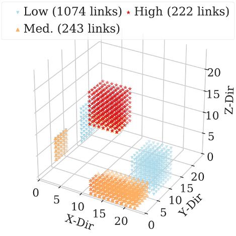
variety of network components (e.g., tiles, NICs) exceeds a         acterization. Data provided or exposed on all Cray Gemini
high-watermark threshold with respect to the ratio of stalls to     systems includes: OS and network performance counter data,
forwarded flits, the software instigates a Congestion Protec-       network resilience-related logs, and workload placement and
tion Event (CPE), which is a throttling of injection of traffic     status logs. In this study, we used five months (Jan 01 to May
from all NICs. The CPE mechanism limits the aggregate traf-         31, 2017) of production network performance-related data
fic injection bandwidth over all compute nodes to less than         (15 TB), network resilience-related logs (100 GB), and appli-
what can be ejected to a single node. While this ensures that       cation placement logs (7 GB). Note that the methodologies
the congestion is at least temporarily alleviated, the network      addressed in this work rely only on the availability of the data,
as a whole is drastically under-subscribed for the duration         independent of the specific tools used to collect the data.
of the throttling. As a result, the performance of all applica-
                                                                    Network Performance Counters: Network performance-
tions running on the system can be significantly impacted.
                                                                    related information on links is exposed via Cray’s gpcdr [35]
Throttling remains active until associated monitored values
                                                                    kernel module. Lustre file system and RDMA traffic in-
and ratios drop below their low-watermark thresholds. Appli-
                                                                    formation is exposed on the nodes via /proc/fs and
cations with sustained high traffic injection rates may induce
                                                                    /proc/kgnilnd. It is neither collected nor made available for
many CPEs, leading to significant time spent in globally throt-
                                                                    analysis via vendor-provided collection mechanisms. On Blue
tling. Bursts of high traffic injection rates may thus trigger
                                                                    Waters, these data are collected and transported off the system
CPEs, due to localized congestion, that could have been alle-
                                                                    for storage and analysis via the Lightweight Distributed Met-
viated without the global negative impact of throttling. There
                                                                    ric Service (LDMS) monitoring framework [17]. In this work,
is an option to enable the software to terminate the applica-
                                                                    we use the following information: directionally aggregated
tion that it determines is the top congestion candidate, though
                                                                    network traffic (bytes and packets) and length of stalls due
this feature is not enabled on the Blue Waters system. The
                                                                    to credit depletion; Lustre file system read and write bytes;
option to terminate application in a production environment
                                                                    and RDMA bytes transmitted and received. LDMS samplers
is not acceptable to most developers and system managers as
                                                                    collect those data at 60-second intervals and calculate derived
it will lead to loss of computational node-hours used by the
                                                                    metrics, such as the percent of time spent in stalls (PT s ) and
application after the last checkpoint.
                                                                    percent of total bandwidth used over the last interval. LDMS
   While some of this congestion may be alleviated by
                                                                    daemons synchronize their sampling to within a few ms (ne-
CEMRs such as feedback of congestion information to appli-
                                                                    glecting clock skew) in order to provide coherent snapshots
cations to trigger rebalancing [29] or to scheduling/resource
                                                                    of network state across the whole system.
managers to preferentially allocate nodes (e.g., via mecha-
nisms such as slurm’s [79] node weight), some may be un-            Network Monitoring Logs: Network failures and conges-
avoidable since all networks have finite bandwidth.                 tion levels are monitored and mitigated by Cray’s xtnlrd soft-
   On Blue Waters a topology-aware scheduling (TAS) [41,            ware. This software further logs certain network events in a
82] scheme is used to decrease the possibility of application       well-known format in the netwatch log file. Significant exam-
communication interference by assigning, by default [12],           ple log lines are provided in Cray documents [33,34]. Regular
node allocations that are constrained within small-convex           expression matching for these lines is implemented in Log-
prisms with respect to the HSN topology. Jobs that exceed           Diver [66], a log-processing tool, which we use to extract the
half a torus will still route outside the allocation and possibly   occurrences, times, and locations of link failures and CPEs.
interfere with other jobs and vice versa; a non-default option
can be used to avoid placement next to such jobs. The I/O           Workload Data: Blue Waters utilizes the Moab scheduler,
routers represent fixed, and roughly evenly distributed, pro-       from which application queue time, start time, end time, exit
portional portions of the storage subsystem. Since the storage      status, and allocation of nodes can be obtained. The work-
subsystem components, including I/O routers, are allocated          load dataset contains information about 815,006 application
(for writes) in a round robin (by request order) manner in-         runs that were executed during our study period. A detailed
dependent of TAS allocations, storage I/O communications            characterization of Blue Waters workloads can be found in
will generally use network links both within and outside the        Appendix B and Blue Waters workload study [58].
geometry of the application’s allocation and can also be a             Note that we will only be releasing network data. Worload
cause of interference between applications.                         data and network monitoring logs will not be released due to
                                                                    privacy and other concerns.
3    Data Sources and Data Collection Tools
  This section describes the datasets and tools used to collect
                                                                    4   CR Extraction and Characterization Tool
data at scale to enable both runtime and long-term characteri-        This section first describes our motivation for choosing
zation of network congestion. We leverage vendor-provided           congestion regions (CRs) as a driver for characterizing net-
and specialized tools to enable collection and real-time stream-    work congestion, and then describes our methodology (imple-
ing of data to a remote compute node for analysis and char-         mented as the Monet tool) for extracting CRs over each data

40   17th USENIX Symposium on Networked Systems Design and Implementation                                     USENIX Association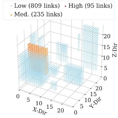
collection interval and the classification of those CRs based each of which ran on 1000 nodes with the same input param-
on severity. eters. We chose NAMD because it consumes approximately
18% of total node-hours available on Blue Waters9 . Figure 4a
4.1 Why Congestion Regions?
shows the execution time of each individual run with respect
We seek to motivate our choice to characterize congestion to the average PT s over all links within the allocated applica-
regions (CRs) and the need for estimates for severity in terms tion topology. (Here we leverage TAS to determine severity
of the stall values. We first show that the charcterization of value estimates based on the values within the allocation; that
hotspot links individually do not reveal the spatial and growth is not a condition for the rest of this work.) Figure 4a shows
characteristics which is needed for diagnosis. Then, we show that execution time is perhaps only loosely related to the av-
how characterizing CRs is meaningful. erage PT s ; with correlation of 0.33 . In contrast, 4b shows
Characterizing hotspot links individually do not reveal the relationship of the application execution time with the
regions of congestion. Figure 3 characterizes the median, maximum average PT s over all CRs (defined in 4.2) within the
99%ile and 99.9%ile duration of the hotspot links by gen- allocated topology; with correlation of 0.89. In this case, exe-
erating the distribution of the duration for which a link per- cution time increases with increasing maximum of average
sists to be in congestion at PT s ≥ PT s Threshold value. For PT s over all regions. We found this relationship to hold for
example, 99.9%ile duration for hotspot links with PT s ≥ 30 other scientific applications. This is a motivating factor for
is 400 minutes (6.67 hours). The measurements show that the the extraction of such congestion regions (CRs) as indicators
median duration of hotspot link at different PT s thresholds of ‘hot-spots’ in the network. We describe the methodology
is constantly at ∼ 0, however, 99.9%ile duration of hotspot for CR extraction in the next section.
links linearly decreases with increasing PT s threshold value. In addition, we selected approximate ranges of PT s values,
Although such characterizations are useful to understand con- corresponding to increasing run times, to use as estimates
gestion at link-level, they hide the spatial characteristics of for the severity levels as these can be easily calculated, un-
congestion such as the existence of multiple pockets of con- derstood and compared. These levels are indicated as sym-
gestion and their spread and growth over time. The lack of bols in the figure. Explicitly, we assign 0-5% average PT s
such information makes it difficult to understand congestion in a CR as Negligible or ‘Neg’, 5-15% as ‘Low’, 15-25% as
characteristics and their root cause. ‘Medium’, and > 25% as ‘High’. These are meant to be quali-
tative assignments and not to be rigorously associated with
a definitive performance variation for all applications in all
Duration (mins)
900
800 median
700 cases, as the network communication patterns and traffic vol-
600 99%ile
500 99.9%ile umes vary among HPC applications. We will use these ranges
400
300 in characterizations in the rest of this work. More accurate
200
100 determinations of impact could be used in place of these in
0
0 10 20 30 40 50 60 70 80 90 100
the future, without changing the validity of the CR extraction
technique.
PTs Threshold (%)
4.2 Extracting Congestion Regions
Figure 3: Duration of congestion on links at different PT s thresholds
We have developed an unsupervised clustering approach
Execution Time (mins)
Execution Time (mins)
550 550
500 500
450
for extracting and localizing regions of congestion in the net-
450
400 Neg
400
350
350 Low
work by segmenting the network into groups of links with
300
Med
300
250
250
200 High similar congestion values. The clustering approach requires
200 150
150 0 5 10 15 20 25 30 35 the following parameters: (a) network graph (G), (b) conges-
0 5 10 15 20 25 30
Avg. PTs across all the links
Max of average PTs across
all regions overlapping the
tion measures (vs for each vertex v in G), (c) neighborhood
within the application topology (%) application topology (%)
distance metric (dδ ), and (d) stall similarity metric (dλ ). The
(a) Not using CRs (b) Using CRs
network is represented as a graph G. Each link in the network
is represented as a vertex v in G, and two vertices are con-
Figure 4: Correlating congestion with NAMD application runtime
nected if the corresponding network links are both connected
CRs captures relationship between congestion-level and to the same switch (i.e., the switch is an edge in the graphs).
application slowdown efficiently. In order to determine For each vertex v, the congestion measures(s) are denoted
possible severity values and show effectiveness of CRs in by the vector vs , which is composed of credit stalls and inq
determining application slowdown, we extracted from the
production Blue Waters dataset a set of NAMD [77]8 runs 9 Thiswas best effort extraction and the NAMD application runs may not
be exactly executing the same binary or processing the same data, as user
8 NAMD has two different implementations: (a) uGNI shared memory parallel may have recompiled the code with a different library or used the same
(SMP)-based, and (b) MPI-based. In this work, unstated NAMD refers to name for dataset while changing the data. There is limited information to
uGNI SMP-based implementation. uGNI is user level Generic Network extract suitable comparable runs from historical data that are also subject to
Interface [83]. allocation and performance variation.
USENIX Association 17th USENIX Symposium on Networked Systems Design and Implementation 41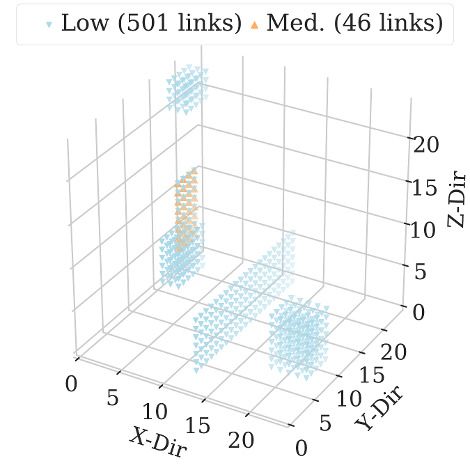
0.27% 0.59
106 0.05
Low 60000
Low
105 Low 0.01 6
104
Med Med 0.3 0.0
#CRs
7
#CRs
High 40000 High
103 0.99 0.38 0.49
102 20000
Neg Med
101 99.33% 2 0.27%
0.1
0
200
400
600
800
1000
1200
1400
1600
100
0.34 0.06
27 28 29 210 211 212 213 214 215 High
CR Size (in terms #links) 0.13% 0.54
CR Duration (mins) (c) CR congestion evolution captures transition probabili-
(b) Distribution of CRs. ties from one severity state to another. Percentage in boxes
(a) Distribution of CR sizes. indicates percentage of total link-hours spent in that state.
Figure 5: CR size, duration, evolution characterization. # of CRs across ‘Low’, ‘Medium’, and ‘High’ are 9.4e05, 7.3e05, and 4.2e05 respectively.
stalls, which we use independently. Distance metrics dδ and conclude that the optimum sliding window time is the knee
dλ are also required, the former for calculating distances be- of the curve drawn between the sliding window time and the
tween two vertices and the latter for calculating differences number of clusters obtained using a clustering algorithm. This
among the stalls vs . We assign each vertex the coordinate decreases truncation errors (in which a cluster is split into
halfway between the logical coordinates of the two switches multiple clusters because of a small sliding window time)
to which that vertex is immediately connected, and we set dδ and collision errors (in which two events not related to each
to be the L1 norm between the coordinates. Since the Blue other merge into a single cluster because of a large sliding
Waters data consists of directionally aggregated information window time). We fixed δ to be 2 in order to consider only
as opposed to counters on a per-tile-link (or buffer) basis, links that are two hops away, to capture the local nature of
then, in our case, dλ is simply the absolute difference between congestion [47]. It should be noted that the region clustering
the two credit-stall or the two inq-stall values of the links, algorithm may discard small isolated regions (size ≤ σ) of
depending on what kinds of regions are being segmented. high congestion. If such CRs do cause high interference, they
We consider credit and inq stalls separately to extract CRs, will grow over time and eventually be captured.
as the relationship between the two types of stalls is not im- Our algorithm works under several assumptions: (a) con-
mediately apparent from the measurements, and thus require gestion spreads locally, and (b) within a CR, the stall values of
two segmentation passes. Next, we outline the segmentation the links do not vary significantly. These assumptions are rea-
algorithm. sonable for k-dimensional toroids that use directional-order
routing algorithm. The methodology used to derive CRs is not
Segmentation Algorithm The segmentation algorithm has
dependent on the resource allocation policy (such as TAS).
four stages which are executed in order, as follows.
The proposed extraction and its use for characterization is
• Nearby links with similar stall values are grouped together.
particularly suitable for analysis of network topologies that
Specifically, they are grouped into the equivalence classes
use directional- or dimensional-order routing. In principle,
of the reflexive and transitive closure of the relation ∼r
the algorithm can be applied to other topologies (such as
defined by x ∼r y ⇔ dδ (x, y) ≤ δ ∧ dλ (xs − ys ) ≤ θ p , where
mesh and high-order torus networks) with other metrics (such
x, y are vertices in G, and δ, θ p are thresholds for distance
as stall-to-flit ratio). Furthermore, the region extraction al-
between vertices and stall values, respectively.
gorithm does not force any shape constraints; thus CRs can
• Nearby regions with similar average stall values, are
be of any arbitrary shape requiring us to store each vertex
grouped together through repetition of the previous step,
associated with the CR. In this work, we have configured the
but with regions in place of individual links. Instead of
tool to store and display bounding boxes over CRs, as doing
using the link values vs , we use the average value of vs over
so vastly reduces the storage requirements (from TBs of raw
all links in the region, and instead of using θ p , we use a
data to 4 MB in this case), provides a succinct summary of
separate threshold value θr .
the network congestion state, and eases visualization.
• CRs that are below the size threshold σ are merged into the
nearest region within the distance threshold δ. We validate the methodology for determining the param-
• Remaining CRs with < σ links are discarded, so that re- eters of the region-based segmentation algorithm and its ap-
gions that are too small to be significant are eliminated. plicability for CR extraction by using synthetic datasets, as
described in Appendix D.
The optimum values for the parameters used in segmenta-
tion algorithms, except for δ, were estimated empirically by 4.3 Implementation and Performance
knee-curve [63] method, based on the number of regions pro-
duced. Using that method, the obtained parameter values 10 We have implemented the region-extraction algorithm as
are: (a) θ p = 4, (b) θr = 4, and (c) σ = 20. In [63], the authors a modified version of the region growth segmentation al-
gorithm [78] found in the open-source PointCloud Library
10 stall
thresholds are scaled by 2.55× to represent the color range (0-255) (PCL) [9] [4]. The tool is capable of performing run-time
for visualization purposes extraction of CRs even for large-scale topologies. Using the
42 17th USENIX Symposium on Networked Systems Design and Implementation USENIX Association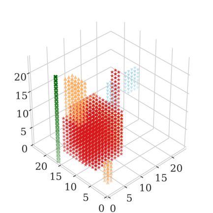
Blue Waters dataset, Monet mined CRs from each 60-second                                                          17%               0.73
                                                                                                    0.2                                           0.16
snapshot of data for 41,472 links in ∼ 7 seconds; Monet was                                                             Low
                                                                                                                 5
running on a single thread of a 2.0 GHz Intel Xeon E5-2683                                                  0.0                             0.1

                                                                                                                            0.05
                                                                                                                                                 3       22%
                                                                                             5%
v3 CPU with 512 GB of RAM. Thus, on Blue Waters Monet                                                                                     0.01
can be run at run-time, as the collection interval is much                                        Neg                                                Med
                                                                                                          0.07
greater than CR extraction time. Since Monet operates on the                               0.69                                                          0.58

                                                                                                                     0.02
                                                                                                                                      1
database, it works the same way whether the data are being                                                                         0.1
                                                                                                    0.04                                         0.27
streamed into the database or it is operating on historical data.                                                       High
                                                                                                                  56%              0.87
5     Characterization Results                                                    Figure 6: Network congestion evolution captures transition probabilities
   In this section, we present results of the application of                      from one severity state to another. Percentage numbers in boxes indicates
                                                                                  percentage of total system wall clock time spent in that state.
our analysis methodology to five months of data from a large-
scale production HPC system (Blue Waters) to provide charac-                      the box next to each state shows the percentage of total link-
terizations of CRs. Readers interested in understanding traffic                   hours13 spent in that state. It can be interpreted as the proba-
characteristics at the link and datacenter-level may refer to a                   bility that a link will be congested at a severity state at a given
related work [16].                                                                time. For example, there is a probability of 0.10% that a link
                                                                                  will be in the ‘High’. These measurements show that:
5.1      Congestion Region Characterization                                       • The vast majority of link-hours (99.3% of total link-hours)
    Here we assess and characterize the congestion severity.                         on Blue Waters are spent in ‘Neg’ congestion. Considera-
                                                                                     tion of a grosser congestion metric, such as the average stall
 CR-level Size and Severity Characterizations: Figure 5a
                                                                                     time across the entire network, will not reveal the presence
 shows a histogram11 of CR sizes in terms of the number of
                                                                                     of significant CRs.
 links for each congested state (i.e., not including ‘Neg’). Fig-
                                                                                  • Once a CR of ‘Low’, ‘Medium’ or ‘High’ congestion is
 ure 5b show a histogram of the durations of CRs across ‘Low’,
                                                                                     formed, it is likely to persist (with a probability of more
‘Medium’ and ‘High’ congestion levels. These measurements
                                                                                     than 0.5) rather than decrease or vanish from the network.
 show that unchecked congestion in credit-based interconnects
 leads to:                                                                        5.2     Network-level Congestion Evolution and
 • High growth and spread of congestion leading to large                                  Transition Probabilities
    CRs. The max size of CRs in terms of number of links                             In this section, we assess and characterize the overall net-
    was found to be 41,168 (99.99% of total links), 6,904                         work congestion severity state. The overall network conges-
    (16.6% of total links), and 2,324 (5.6% of total links) across                tion severity state is the state into which the highest CR falls.
   ‘Low’, ‘Medium’ and ‘High’ congestion levels respectively,                     That assignment is independent of the overall distribution
    whereas the 99th percentile of the12 CR size was found to                     of links in each state. Figure 6 shows the probabilities that
    be 299, 448, and 214 respectively.                                            transitions between network states will occur between one
 • Localized congestion hotspots, i.e., pockets of congestion.                    measurement interval and the next. The rectangular boxes in
    CRs rarely spread to cover all of the network. The number                     the figure indicate the fraction of time that the network resides
    of CRs decreases (see Figure 5a) with increasing size across                  in each state. These measurements show the following:
    all severity states except for ‘Low’ for which we observe                     • While each individual link of the entire network is most
    increase at the tail. For example, there are ∼16, 000 CRs in                     often in a state of ‘Neg’ congestion, there exists at least one
    the ‘High’ which comprise 128 links but only ∼ 141 CRs                          ‘High’ CR for 56% of the time. However, ‘High’ CRs are
    of size ∼ 600.                                                                   small; in Section 5.1, we found that 99th percentile size of
 • Long-lived congestion. The CR count decreases with in-                           ‘High’ is 214 links. Thus, the Blue Waters network state is
    creasing duration, however there are many long-lived CRs.                        nearly always non-negligible (95%), with the “High” state
    The 50%ile, 99%ile and max duration of CRs across all                            occurring for the majority of the time.
    states were found to be 579 minutes (9.7 hours), 1421 min-                    • There is a significant chance that the current network state
    utes (23.6 hours), and 1439 minutes (24 hours) respectively,                     will persist or increase in severity in the next measurement
    whereas the 50%ile, 99%ile and max PT s of CRs was found                         period. For example, there is an 87% chance that it will
    to be 14%, 46%, and 92%, respectively. CR duration did not                       stay in a ‘High’ state.
    change significantly across ‘Low’, ‘Medium’, and ‘High’.                      • A network state is more likely to drop to the next lower
CR Evolution and State Probability: Figure 5c shows the                              state than to drop to ‘Neg’.
transition probabilities of the CR states. The percentage in                      • Together these factors indicate that congestion builds and
                                                                                     subsides slowly, suggesting that it is possible to fore-
11 plotted  as lines and every tenth point marked on the line using a shape for
                                                                                  13 Link-hours
   clarity.                                                                                         are    calculated     by                ∑ (#links in Region) ×
12 We will use %ile to denote percentile in the rest of the paper.                  (measurement time-window) for each state.

USENIX Association                                       17th USENIX Symposium on Networked Systems Design and Implementation                                   43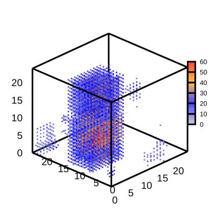
cast (within bounds) congestion levels. Combined with
  proactive localized congestion mitigation techniques and
  CEMRs, such forecasts could significantly improve overall                                  System Load
  system performance and application throughput.                                               Changes

5.3    Application Impact of CR                                                                    (a)
                                                                                                                              (b)

   The potential impact of congestion on applications can be
significant, even when the percentage of link-hours spent in
non-‘Neg’ congested regions is small. While we cannot quan-
tify congestion’s impact on all of the applications running on
Blue Waters (as we lack ground truth information on particu-
lar application runtimes without congestion), we can quantify                                        (d)                      (c)
the impact of congestion on the following:
• Production runs of the NAMD application [77]. The worst-
                                           such as system load
                                            (i) System reasons

   case NAMD execution runtime was 3.4× slower in the
   presence of high CRs relative to baseline runs (i.e., negli-
   gible congestion). The median runtime was found be 282
   minutes, and hence worst-case runtime was 1.86× slower
   than the median runtime. This is discussed in more detail                                    Link Failure
   in Section 4.1.
• In [16], authors show that benchmark runs of PSDNS [74]
   and AMR [2] on 256 nodes slowed down by as much as
                                                                                                     Change in traffic
   1.6× even at low-levels of congestion (5% < PT s ≤ 15%).                                             volume
                                        (ii) Network link

   To find a upper bound on the number of potentially im-
                                              Failure

pacted applications, we consider the applications whose allo-
cations are directly associated with a router in a CR. Out of
815,006 total application runs on Blue Waters, over 16.6%,
12.3%, and 6.5% of the unique application runs were impacted
by ‘Low’, ‘Medium’, and ‘High’ CRs, respectively.
                                           pattern within an application
                                           (iii) Change in comm. traffic

                                                                           Figure 7: Case studies: network congestion is shown due to (i) sys-
5.4    Congestion Scenarios                                                tem issues (such as introduction of new applications), (ii) failures
                                                                           (such as network link failure), and (iii) change in communication
   In this section, we show how CRs manifest under differ-
                                                                           pattern within the application.
ent congestion scenarios: (a) system issues (e.g. changes in
system load), (b) network-component failures (e.g. link fail-              occurred (Figure 7(i)(b,c)). The ‘High’ (red) 14 and ‘Medium’
ures), and (c) intra-application contention. Since the CRs are             (orange) severity CRs overlapped with the applications.
described as bounding boxes with coordinates described in                     The increase in the severity of congestion was due to high
relation to the 3D torus, they can easily be visualized in con-            I/O bandwidth utilization by the Variant Calling application.
junction with applications’ placements at runtime on the torus.            The overall network state remained ‘High’ for ∼ 143 minutes
CRs of ‘Neg’ congestion are not shown in the figures.                      until the Variant Calling application completed. At that time,
Congestion due to System Issues: Network congestion                        the congestion subsided, as shown in Figure 7(i)(d).
may result from contention between different applications                  Congestion Due to Network-component Failures:
for the same network resources. That can occur because of                  Network-related failures are frequent [55, 68] and may
a change in system load (e.g. launches of new applications)                lead to network congestion, depending on the traffic on
or change in application traffic that increases contention on              the network and the type of failure. In [55], the mean time
shared links between applications.                                         between failures (MTBF) for directional links in Blue Waters
   Figure 7(i) shows four snapshots, read clockwise, of ex-                was found to be approximately 2.46e06 link-hours (or 280
tracted CRs, including size and severity state, for different              link-years). Given the large number of links (41,472 links) on
time intervals during a changing workload. Figure 7(i)(a)                  Blue Waters, the expected mean time between failure of a
shows that ‘Low’ (blue) CRs when most of the workload con-                 link across the system is about 59.2 hours; i.e., Blue Waters
sists of multiple instances of MPI-based NAMD [77]. The                    admins can expect one directional-link failure every 59.2
overall network state was thus ‘Low’. The CRs remained rela-               hours.
tively unchanged for 40 minutes, after which two instances                    Failures of directional links or routers generally lead to
of NAMD completed and Variant Calling [37] was launched.
Three minutes after the launch, new CRs of increased severity              14 not   visible and hidden by other regions.

44    17th USENIX Symposium on Networked Systems Design and Implementation                                                 USENIX Association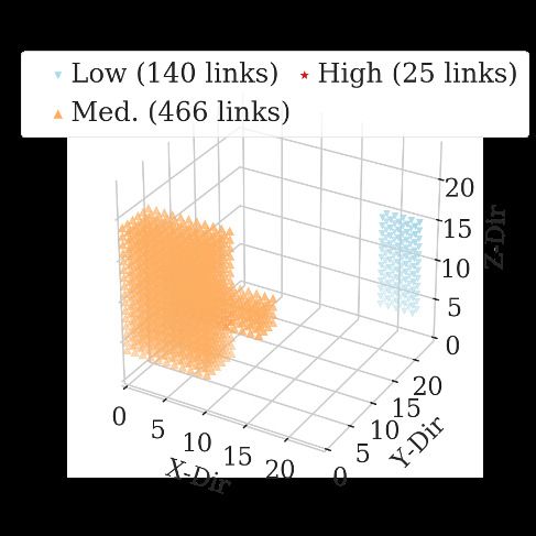
occurrences of ‘High’ CRs, while isolated failures of a few
switch links (which are much more frequent) generally do not
lead to occurrences of significant CRs. In this work we found
that 88% of directional link failures led to congestion; how-
ever, isolated failures of switch links did not lead to significant
CRs (i.e., had ‘Neg’ CRs).
                                                                      (a) Box plot of duration of throttling   (b) Box plot of time between triggers
   Figure 7(ii) shows the impact of a network blade failure                                                    of congestion mitigation events
that caused the loss of two network routers and about 96                  Figure 8: Characterizing Cray Gemini congestion mitigation events.
links (x,y,z location of failure at coordinates (12,3,4) and
(12,3,3)). Figure 7(ii)(a) shows the congestion CRs before            6     Using Characterizations: Congestion Re-
the failure incident and Figure 7(ii)(b) shows the CRs just                 sponse
after the completion of the network recovery. Immediately                In this section, we first discuss efficacy of Cray CPEs and
after failure, the stalls increased because of the unavailability     then show how our CR-based characterizations can be used to
of links, requiring the packets to be buffered on the network         inform effective responses to performance-degrading levels
nodes. The congestion quickly spread into the geometry of             of congestion.
nearby applications in the torus. Failure of a blade increased
the overall size (in number of links) of ‘Low’ CRs by a factor        Characterizing Cray CPEs: Recall from Section 2 that the
of 2, and of ‘Medium’ CRs by a factor of 4.2, and created             vendor-provided congestion mitigation mechanism throttles
previously non existent ‘High’ CRs with more than 200 links.          all NIC traffic injection into the network irrespective of the
                                                                      location and size of the triggering congestion region. This
Congestion Due to Intra-Application Issues: Conges-                   mitigation mechanism is triggered infrequently by design and
tion within an application’s geometry (intra-application con-         hence may miss detections and opportunities to trigger more
tention) can occur even with TAS. Figure 7(iii) shows con-            targeted congestion avoidance mechanisms. On Blue Waters,
gestion CRs while the uGNI-based shared memory parallel               congestion mitigation events are generally active for small
(SMP) NAMD application on more than 2,000 nodes. The                  durations (typically less than a minute), however, in extreme
application is geometrically mapped on the torus starting at          cases, we have seen them active for as long as 100 minutes.
coordinates (15, 18, 0) and ending at coordinates (1, 21, 23)         Each throttling event is logged in netwatch log files.
(wrapping around). The congestion CRs alternate between the              We define a congestion mitigation event (CME) as a col-
two states shown (state 1 shown in Figure 7(iii)(a), and state 2,     lection of one or more throttling events that were coalesced
shown in Figure 7(iii)(b)) throughout the application run-time        together based on a sliding window algorithm [63] with a slid-
because of changes in communication patterns corresponding            ing window of 210 seconds, and we use this to estimate the
to the different segments of the NAMD code.                           duration of the vendor-provided congestion mitigation mech-
                                                                      anisms. Figure 8a and 8b shows a box plot of duration of
   Intra-application contention is less likely to elevate to
                                                                      and time between CMEs respectively. The analysis of CMEs
cause global network issue, unless the links are involved in
                                                                      shows that :
global (e.g., I/O) routes, or if the resulting congestion is heavy
                                                                      • CMEs were triggered 261 times; 29.8% of which did not
enough to trigger the system-wide mitigation mechanism (see
                                                                         alleviate congestion in the system. Figure 9 shows a case
Section 2.2).
                                                                         where the size and severity of CRs increases after a series
Importance of diagnosis: In this section, we have iden-                  of throttling events.
tified three high-level causes of congestion, which we cat-           • The median time between triggers of CMEs was found to
egorize as (a) system issues, (b) network-component fail-                be 7 hours. The distribution of time between events is given
ures, and (c) intra-application contention. For each cause,              in Figure 8b.
system managers could trigger one of the following actions            • CMEs are generally active for small durations (typically
to reduce/manage congestion. In the case of intra-application            less than a minute), however, in extreme cases, we have
congestion, an automated MPI rank remapping tool such as                 seen them active for as long as 100 minutes.
TopoMapping [46], could be used to change traffic flow band-          • 8% of the application runs were impacted with over 700 of
width on links to reduce congestion on them. In the case                 those utilizing > 100 nodes.
of inter-application congestion (caused by system issues or              These observations motivate the utility of augmenting the
network failures), a node-allocation policy (e.g., TAS) could         vendor supplied solution of global traffic suppression to man-
use knowledge of congested regions to reduce the impact of            age exceptionally high congestion bursts with our more local-
congestion on applications. Finally, if execution of an appli-        ized approach of taking action on CRs at a higher system-level
cation frequently causes inter-application congestion, then           of granularity to alleviate sources of network congestion.
the application should be re-engineered to limit chances of           CR-based congestion detection to increase mitigation ef-
congestion.                                                           fectiveness: CR based characterizations can potentially im-

USENIX Association                              17th USENIX Symposium on Networked Systems Design and Implementation                             45
Low (347 links) Med. (77 links) Low (174 links) High (969 links)
and potential offenders for further analysis. We can combine
Med. (150 links)
system information with the CR-characterizations to help
20 20
diagnose causes of significant congestion. Factors include
applications that inject more traffic than can be ejected into
Z-Dir
Z-Dir
15 15
10 10 the targets or than the traversed links can transfer, either via
5 5
communication patterns (e.g., all-to-all or many-to-one) or
0 0
20 20
I/O traffic, and link failures. These can typically be identified
0
5
15
10
0
5
15
10
by observation(s) of anomalies in the data.
ir
ir
10 10
-D
-D
15 5 15 5
Y
Y
X- X-
Di
r
20
0
Di
r
20
0 Mining Candidate Congestion-Causing Factors For
(a) Congestion before triggering of (b) Congestion after 30 minutes of
CPE CPE
each congestion Region, CRi , identified at time T , we cre-
ate two tables ACRi (T ) and FCRi (T ), as described below.
Figure 9: A case in which a congestion protection event (CPE)
failed to mitigate the congestion ACRi (T ) table: Each row in ACRi (T ) corresponds to an ap-
plication that is within Nhops ≤ 3 hops away from the bound-
prove congestion mitigation and CEMR effectiveness by more
ing box of the congestion region CRi . ACRi (T ) contains in-
accurately determining which scenarios should be addressed
formation about the application and its traffic characteristics
by which mechanisms and by using the identified CRs to
across seven traffic features: (a) application name, (b) max-
trigger localized responses more frequently than Cray CMEs.
imum read bytes per minute, (c) maximum write bytes per
That approach is motivated by our discovery (see Section 5.2)
minute, (d) maximum RDMA read bytes per minute, (e) max-
that the network is in a ‘High’ congestion state the major-
imum RDMA write bytes per minute, (f) maximum all-to-all
ity of the time, primarily because of CRs of small size but
communication traffic bytes per minute, and (g) maximum
significant congestion severity.
many-to-one communication traffic bytes per minute, where
We define a Regions Congestion Event (RCE) as a time-
the maximums are taken over the past 30 minutes, i.e., the
window for which each time instance has at least one region of
most recent 30 measurement windows. The list of applica-
‘High’ congestion. We calculate it by combining the CR eval-
tions that are within Nhops away from congestion region CRi
uations across 5-minute sliding windows. Figure 10 shows
are extracted from the workload data. The measurements for
boxplots of (a) average credit PT S across all extracted CRs
features (a) to (e) are extracted by querying network perfor-
during RCEs’, (b) average inq PT S across all RCEs’, (c) times
mance counter data, whereas we estimate the features (f) and
between RCE, and (d) durations of the RCEs’. These mea-
(g) are estimated from Network performance counter data
surements show
by taking several bisection cuts over the application geome-
• Relative to the vendor-provided congestion mitigation
try and comparing node traffic ingestion and ejection bytes
mechanisms, our characterization results in 13× more
among the two partitions of the bisection cut.
events (3390 RCEs) upon which we could potentially act.
FCRi (T ) table: Each row in FCRi (T ) corresponds to an
• Vendor provided congestion mitigation mechanisms trigger
application that is within Nhops ≤ 3 away from the congestion
on 8% (261 of 3390) of RCEs.
boundary of CRi . FCRi (T ) contains information about failure
• The average PT S of maximum inq- and credit-stall across
events across three failure features: (a) failure timestamp, (b)
all extracted regions present in RCEs is quite high, at 33.8%
failure location (i.e., coordinates in the torus), and (c) failure
and 27.4%, respectively.
type (i.e., switch link, network link, and router failures). Lists
• 25% of 3390 RCEs lasted for more than 30 minutes, and
of failure events that are within Nhops away from congestion
the average duration was found to be approximately an
region CRi are extracted from network failure data.
hour.
CRs discovery could also be used for informing conges- Identifying Anomalous or Extreme Factors: The next
tion aware scheduling decisions. Communication-intensive step is to identify extreme application traffic characteris-
applications could be preferentially placed to not contend for tics or network-related failures over the past 30 minutes that
bandwidth in significantly congested regions or be delayed have led to the occurrence of CRs. For each traffic feature
from launching until congestion has subsided. in ACRi (T ), we use an outlier detection method to identify
the top k applications that are exhibiting anomalous behavior.
7 Using Characterizations: Diagnosing The method uses the numerical values of the features listed in
Causes of Congestion table ACRi (T ). Our analysis framework uses a median-based
Section 5.4 identifies the root causes of congestion and outlier detection algorithm proposed by Donoho [40] for each
discusses the the importance of diagnosis. Here we explore CRi . According to [40], the median-based method is more ro-
that idea to create tools to enable diagnosis at runtime. bust than mean-based methods for skewed datasets. Because
CRs due to network-related failure events 15 are rare relative
7.1 Diagnosis Methodology and Tool
to congestion caused by other factors, all failure events that
We present a methodology that can provide results to help
draw a system manager’s attention to anomalous scenarios 15 In this paper, we do not consider the effect of lane failures on congestion.
46 17th USENIX Symposium on Networked Systems Design and Implementation USENIX Association(a)Boxplot of average credit (b) Boxplot of average inq- (c)Boxplot of time between (d) Boxplot of duration of con-
stall across extracted conges- stall across extracted conges- congestion events. gestion.
tion events. tion events.
Figure 10: Characterization of Regions Congestion Events (RCE).
occur within Nhops of CRi in the most recent 30 measurement congestion regions (see the top-right graph in Figure 11(a)).
windows are marked as anomalous. Step 2. Congestion diagnosis. There are 3 steps associated
Generating Evidence: The last step is to generate evidence with diagnosing the cause of the congestion.
for determining whether anomalous factors identified in the Step 2.1. Mining candidate factors. To determine the cause
previous step are truly responsible for the observed congestion of the congestion, we correlated the CR-data with application-
in the CR. The evidence is provided in the form of a statis- related network traffic (for all applications that overlapped
tical correlation taken over the most recent 30 measurement with or were near the congestion regions) and network in-
time-windows between the moving average stall value of the formation to generate candidate factors that may have led to
links and the numerical traffic feature(s) obtained from the congestion. In this example, there were no failures; hence, this
data (e.g., RDMA read bytes per minute of the application) analysis generated only application-related candidate factors
associated with the anomalous factor(s). For failure-related ACRi , as shown in Figure 11.
anomalous factors, we calculate the correlation taken over Step 2.2. Identifying anomalous factors. Next, we utilized
the most recent 30 measurement time-windows between the the application traffic characteristics from candidate factors
moving average of observed traffic summed across the links observed over the last 30 minutes (i.e., many-to-one or all-to-
that are within Nhops away from the failed link(s) and the stall all traffic communication, and file system statistics such as
values16 . A high correlation produces the desired evidence. read or write bytes) to identify anomalous factors by using
We order the anomalous factors using the calculated correla- a median-based outlier detection algorithm. In our example,
tion value regardless of the congestion cause. Additionally, as indicated in Figure 11(b), the offending application was
we show a plot of stall values and the feature associated with “Enzo” which was running on 32 nodes allocated along the “Z”
the anomalous factor(s) to help understand the impact of the direction at location (X,Y,Z) = (0,16,16) (indicated by a black
anomalous factor(s) on congestion. circle in Figure 11(a)). At the time of detection, “Enzo” was
The steps in this section were only tested on a dataset reading from the file system at an average rate of 4 GB/min
consisting of the case studies discussed in Section 5.4 and 7 (averaged over past 30 minutes and with a peak rate of 70
because of lack of ground truth labels on root causes. Creation GB/min), which was 16x greater than the next-highest rate
of labels on congestion causes requires significant human ef- of read traffic by any other application in that time-window.
fort and is prone to errors. However, we have been able to The ACRi (T ) for RDMA read bytes/min was 70 GB/min.
generate labels by using the proposed unsupervised method- The tool identified the RDMA read bytes/min of the “Enzo”
ology, which provides a good starting point for diagnosis. application as the outlier feature. Hence, “Enzo” was marked
as the anomalous factor that led to the congestion.
7.2 Comprehensive Congestion Analysis Step 2.3. Generating evidence. Once the potential cause
In this section, we describe an example use case in which had been established, further analysis produced additional
our analysis methodologies were used to detect and diagnose evidence (e.g., distribution and correlation coefficient asso-
the congestion in a scenario obtained from real data for which ciated with link stalls in the congestion time window) to
the ground truth of the cause was available. The overall steps validate/verify the diagnosis results produced in Step 2.2.
involved in using our methodologies, included in our Monet Figure 11(c), in the top graph, shows a plot of the sum of
implementation, for congestion detection and diagnosis are stall rates on all links for all the Gemini routers local to the
summarized in Figure 11 and described in Section 7. Not all compute nodes used by the offending application, (i.e., Enzo)
of the steps discussed below are currently automated, but we (normalized to the total stall rate throughout the duration of
are working on automating an end-to-end pipeline. the application run). The two peaks (marked) in this top plot
Step 1. Extraction of CR. Figure 11(a) shows that our anal- correspond to the increase in read bytes (normalized to total
ysis indicated wide spread high-level congestion across the read bytes during the application run) shown in the bottom
system (see the left graph in Figure 11(a)). An in-depth anal- plot. Note that abnormal activity (an excessive amount of traf-
ysis of the raw data resulted in identification/detection of fic to the file system) occurred around 10:10 AM (as shown
16 Increase in traffic near a failed link leads to congestion as shown in Sec- Figure 11(c)), which was about 20 minutes before the severe
tion 5.4. congestion developed in the system (seen in Figure 11(a)). A
USENIX Association 17th USENIX Symposium on Networked Systems Design and Implementation 47You can also read