In Silico Labeling: Predicting Fluorescent Labels in Unlabeled Images - Stanford ...
←
→
Page content transcription
If your browser does not render page correctly, please read the page content below
Resource

In Silico Labeling: Predicting Fluorescent Labels in
Unlabeled Images
Graphical Abstract                                                          Authors
    Pairs of transmitted light z-stacks      Untrained         Predicted    Eric M. Christiansen, Samuel J. Yang,
      and fluorescence image sets          neural network    fluorescence   D. Michael Ando, ..., Lee L. Rubin,
                                                                images      Philip Nelson, Steven Finkbeiner

                                                                            Correspondence
                                                                            ericmc@google.com (E.M.C.),
                                                                            pqnelson@google.com (P.N.),
                                                                            sfinkbeiner@gladstone.ucsf.edu (S.F.)
                                              Trained
                                           neural network                   In Brief
                                                                            In silico labeling, a machine-learning
                                                                            approach, reliably infers fluorescent
                                                                            measurements from transmitted-light
                                                                            images of unlabeled fixed or live
                                                                            biological samples.
                                           New transmitted
                                            light z-stack

Highlights
d    Fluorescence microscopy images can be predicted from
     transmitted-light z stacks

d    7 fluorescent labels were validated across three labs,
     modalities, and cell types

d    New labels can be predicted using minimal additional
     training data

              Christiansen et al., 2018, Cell 173, 1–12
              April 19, 2018 ª 2018 Elsevier Inc.
              https://doi.org/10.1016/j.cell.2018.03.040
Please cite this article in press as: Christiansen et al., In Silico Labeling: Predicting Fluorescent Labels in Unlabeled Images, Cell (2018),
 https://doi.org/10.1016/j.cell.2018.03.040

Resource

In Silico Labeling: Predicting
Fluorescent Labels in Unlabeled Images
Eric M. Christiansen,1,11,* Samuel J. Yang,1 D. Michael Ando,1,9 Ashkan Javaherian,2,9 Gaia Skibinski,2,9
Scott Lipnick,3,4,8,9 Elliot Mount,2,10 Alison O’Neil,3,10 Kevan Shah,2,10 Alicia K. Lee,2,10 Piyush Goyal,2,10
William Fedus,1,6,10 Ryan Poplin,1,10 Andre Esteva,1,7 Marc Berndl,1 Lee L. Rubin,3 Philip Nelson,1,*
and Steven Finkbeiner2,5,*
1Google,  Inc., Mountain View, CA 94043, USA
2Taube/Koret   Center for Neurodegenerative Disease Research and DaedalusBio, Gladstone Institutes, San Francisco, CA 94158, USA
3Department of Stem Cell and Regenerative Biology, Harvard University, Cambridge, MA 02138, USA
4Department of Biomedical Informatics, Harvard Medical School, Boston, MA 02115, USA
5Departments of Neurology and Physiology, University of California, San Francisco, 94158, USA
6Montreal Institute of Learning Algorithms, University of Montreal, Montreal, QC, Canada
7Department of Electrical Engineering, Stanford University, Stanford, CA 94305, USA
8Center for Assessment Technology and Continuous Health, Massachusetts General Hospital, Boston, MA 02114, USA
9These authors contributed equally
10These authors contributed equally
11Lead Contact

*Correspondence: ericmc@google.com (E.M.C.), pqnelson@google.com (P.N.), sfinkbeiner@gladstone.ucsf.edu (S.F.)
 https://doi.org/10.1016/j.cell.2018.03.040

SUMMARY                                                                  unprecedented opportunities to reveal macromolecular struc-
                                                                         tures, metabolites, and other subcellular constituents.
Microscopy is a central method in life sciences. Many                       Nevertheless, fluorescence labeling has limitations. Specificity
popular methods, such as antibody labeling, are                          varies; labeling is time consuming; specialized reagents are
used to add physical fluorescent labels to specific                      required; labeling protocols can kill cells; and even live cell pro-
cellular constituents. However, these approaches                         tocols can be phototoxic. The reagents used for immunocyto-
have significant drawbacks, including inconsistency;                     chemistry commonly produce non-specific signals because of
                                                                         antibody cross-reactivity, have significant batch-to-batch vari-
limitations in the number of simultaneous labels
                                                                         ability, and have limited time windows for image acquisition in
because of spectral overlap; and necessary pertur-
                                                                         which they maintain signal. Lastly, measuring the label requires
bations of the experiment, such as fixing the cells,                     an optical system that can reliably distinguish it from other sig-
to generate the measurement. Here, we show that a                        nals in the sample while coping with fluorophore bleaching.
computational machine-learning approach, which                              We hypothesized that microscopic images of unlabeled cells
we call ‘‘in silico labeling’’ (ISL), reliably predicts                  contain more information than is readily apparent, information
some fluorescent labels from transmitted-light im-                       that traditionally requires immunohistochemistry to reveal. To
ages of unlabeled fixed or live biological samples.                      test this, we leveraged major advances in deep learning (DL), a
ISL predicts a range of labels, such as those for                        type of machine learning that has resulted in deep neural net-
nuclei, cell type (e.g., neural), and cell state (e.g.,                  works capable of superhuman performance on specialized tasks
cell death). Because prediction happens in silico,                       (Schroff et al., 2015; Silver et al., 2016; Szegedy et al., 2016). Prior
                                                                         work using deep learning to analyze microscopy images has been
the method is consistent, is not limited by spectral
                                                                         limited, often relying on known cell locations (Held et al., 2010;
overlap, and does not disturb the experiment. ISL
                                                                         Zhong et al., 2012) or the imposition of special and somewhat arti-
generates biological measurements that would                             ficial sample preparation procedures, such as the requirement for
otherwise be problematic or impossible to acquire.                       low-plating density (Held et al., 2010; Van Valen et al., 2016;
                                                                         Zhong et al., 2012). As such, it is unclear whether deep learning
INTRODUCTION                                                             approaches would provide a significant and broad-based
                                                                         advance in image analysis and are capable of extracting useful,
Microscopy offers a uniquely powerful way to observe cells and           not readily apparent, information from unlabeled images.
molecules across time and space. However, visualizing cellular              Here, we sought to determine if computers can find and pre-
structure is challenging, as biological samples are mostly water         dict features in unlabeled images that normally only become
and are poorly refractile. Optical and electronic techniques             visible with invasive labeling. We designed a deep neural
amplify contrast and make small signals visible to the human             network and trained it on paired sets of unlabeled and labeled
eye, but resolving certain structural features or functional char-       images. Using additional unlabeled images of fixed or live cells
acteristics requires different techniques. In particular, fluores-       never seen by the network, we show it can accurately predict
cence labeling with dyes or dye-conjugated antibodies provides           the location and texture of cell nuclei, the health of a cell, the

                                                                                        Cell 173, 1–12, April 19, 2018 ª 2018 Elsevier Inc. 1
Please cite this article in press as: Christiansen et al., In Silico Labeling: Predicting Fluorescent Labels in Unlabeled Images, Cell (2018),
 https://doi.org/10.1016/j.cell.2018.03.040

          A

                                                                                                     B                                E

                                                                                                     C

                                                                                                     D

Figure 1. Overview of a System to Train a Deep Neural Network to Make Predictions of Fluorescent Labels from Unlabeled Images
(A) Dataset of training examples: pairs of transmitted-light images from z-stacks of a scene with pixel-registered sets of fluorescence images of the same scene.
The scenes contain varying numbers of cells; they are not crops of individual cells. The z-stacks of transmitted-light microscopy images were acquired with
different methods for enhancing contrast in unlabeled images. Several different fluorescent labels were used to generate fluorescence images and were varied
between training examples; the checkerboard images indicate fluorescent labels that were not acquired for a given example.
(B) An unfitted model comprising a deep neural network with untrained parameters.
(C) A fitted model was creating by fitting the parameters of the untrained network (B) to the data (A).
(D) To test whether the system could make accurate predictions from novel images, a z-stack of images from a novel scene was generated with one of the
transmitted-light microscopy methods used to produce the training dataset (A).
(E) The trained network, C, was used to predict fluorescence labels learned from (A) for each pixel in the novel images (D). The accuracy of the predictions was
then evaluated by comparing the predictions to the actual images of fluorescence labeling from (D) (data not shown).
See also Figure S6 and Table S1.

type of cell in a mixture, and the type of subcellular structure. We              training examples, consisting of pairs of transmitted-light z-stack
also show that the trained network exhibits transfer learning:                    images and fluorescence images that are pixel registered. The
once trained to predict a set of labels, it could learn new labels                training pairs come from numerous experiments across various
with a small number of additional data, resulting in a highly                     labs, samples, imaging modalities, and fluorescent labels. This
generalizable algorithm, adaptable across experiments.                            is a means to improve the network via multi-task learning: having
                                                                                  it learn across several tasks (Figure 1A). Multi-task learning can
RESULTS                                                                           improve networks when the tasks are similar, because common
                                                                                  features can be learned and refined across the tasks. We chose
Training and Testing Datasets for Supervised Machine                              deep neural networks (Figure 1B) as the statistical model to learn
Learning                                                                          from the dataset because they can express many patterns and
To train a deep neural network to predict fluorescence images                     result in systems with substantially superhuman performance.
from transmitted-light images, we first created a dataset of                      We trained the network to learn the correspondence rule

2 Cell 173, 1–12, April 19, 2018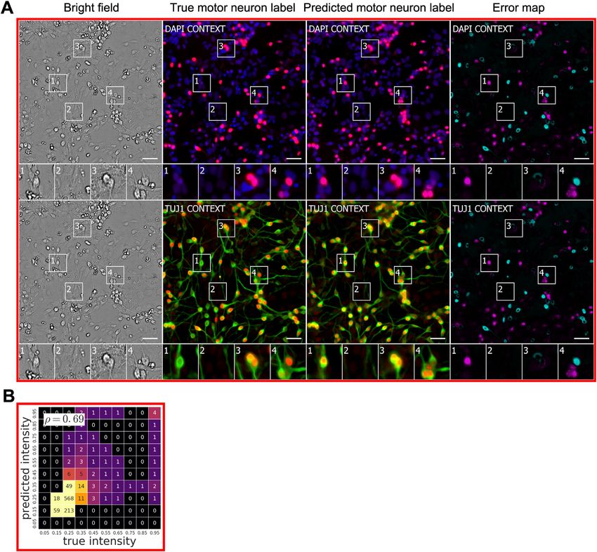
Please cite this article in press as: Christiansen et al., In Silico Labeling: Predicting Fluorescent Labels in Unlabeled Images, Cell (2018),
 https://doi.org/10.1016/j.cell.2018.03.040

(Figure 1C) - a function mapping from the set of z-stacks of trans-      that operates on a large length-scale in a broad region around
mitted-light images to the set of images of all fluorescent labels       the center of the network’s input, and three paths in between.
in the training set. If our hypothesis is correct, the trained network   Inspired by U-Net (Ronneberger et al., 2015) and shown in the
would examine an unseen z-stack of transmitted-light images              leftmost path of Figure 3 in Data S1, the computational path
(Figure 1D) and generate images of corresponding fluorescent             with the finest detail stays at the original length scale of the input
signals (Figure 1E). Performance is measured by the similarity           so that local information can flow from the input to the output
of the predicted fluorescence images and the true images for             without being blurred. Multi-scale architectures are common in
held-out examples.                                                       animal vision systems and have been reported to be useful in
   The training datasets (Table 1) include different cell types with     vision networks (Farabet et al., 2013). We took a multi-scale
different labels made by different laboratories. We used human           approach (Farabet et al., 2013), in which intermediate layers at
motor neurons from induced pluripotent stem cells (iPSCs), pri-          multiple scales are aligned by resizing, but used transposed con-
mary murine cortical cultures, and a breast cancer cell line.            volutions (Zeiler et al., 2010) to learn the resizing function rather
Hoechst or DAPI was used to label cell nuclei; CellMask was              than fixing it like in Farabet et al. (2013). This lets the network
used to label plasma membrane; and propidium iodide was                  learn the spatial interpolation rule that best fits its task.
used to label cells with compromised membranes. Some cells                  The network is composed of repeated modules, as in the pop-
were immunolabeled with antibodies against the neuron-specific           ular Inception network used in computer vision (Szegedy et al.,
b-tubulin III (TuJ1) protein, the Islet1 protein for identifying motor   2015a), but with the Inception module optimized for performance
neurons, the dendrite-localized microtubule associated pro-              (STAR Methods; Figure 2 in Data S1) using Google Hypertune
tein-2 (MAP2), or pan-axonal neurofilaments.                             (Golovin et al., 2017). Hypertune is an automatic function opti-
   To improve the accuracy of the network, we collected multiple         mizer that tries to find a minimum of a function in a bounded
transmitted-light images with varying focal planes. Monolayer            space. We expressed module design choices as parameters
cultures are not strictly two dimensional, so any single image           and the prediction error as the function to be optimized, and
plane contains limited information about each cell. Translating          used Hypertune to select the design, optimizing over the training
the focal plane through the sample captures features that are            dataset, with the test set withheld.
in sharp focus in some images while out of focus in others (Fig-            The learned part of the deep neural network is primarily made
ure 1 in Data S1). Normally, out-of-focus features are undesir-          up of convolutional kernels, small filters that convolve over prior
able, but we hypothesized the implicit three-dimensional infor-          layers to compute the next layers. These kernels are restricted to
mation in these blurred features could be an additional source           the interiors of the input layers (i.e., the convolutions are valid or
of information. We, thus, collected sets of images (z-stacks) of         not zero-padded) (Table S1) (Dumoulin and Visin, 2016), making
the same microscope field from several planes at equidistant             the network approximately translation invariant. As such, each
intervals along the z axis and centered at the plane that was            predicted pixel of the network’s final output is computed by
most in-focus for the majority of the cell bodies.                       approximately the same function, but using different input
   During collection, the microscope stage was kept fixed in             data, improving the scalability and accuracy while minimizing
x and y, while all images in a set were acquired, to preserve            boundary effects.
(x, y) registration of pixels between the transmitted-light and fluo-       We implemented the network in TensorFlow (Abadi et al.,
rescence images (Figure 2; Table 1).                                     2015), a popular open-source library for deep learning. It was
                                                                         trained using the Adam optimizer (Kingma and Ba, 2014), a
Developing Predictive Algorithms with Machine                            commonly used gradient-based function optimizer included in
Learning                                                                 TensorFlow.
With these training sets, we used supervised machine learning               The final network (STAR Methods) produces a discrete prob-
(ML) (Table S1) to determine if predictive relationships could be        ability distribution over 256 intensity values (corresponding to
found between transmitted-light and fluorescence images of               8-bit pixels) for each pixel of the output image. It reads z-stacks
the same cells. We used the unprocessed z-stack as input for             of transmitted-light images collected with bright field, phase
machine-learning algorithm development. The images were                  contrast, or differential interference contrast methods and out-
preprocessed to accommodate constraints imposed by the                   puts simultaneous predictions for every label kind that appeared
samples, data acquisition, and the network. For example, we              in the training datasets. It achieves a lower loss on our data than
normalized pixel values of the fluorescence images (STAR                 other popular models while using fewer parameters (Figure S4B;
Methods) as a way to make the pixel-prediction problem well              STAR Methods).
defined. In addition, we aimed to predict the maximum projec-
tion of the fluorescence images in the z axis. This was to account       Network Predictions of Cell Nuclei
for the fact that pairs of transmitted and fluorescence images           We asked whether we could train a network to predict the label-
were not perfectly registered along the z axis and exhibited dif-        ing of cell nuclei with Hoechst or DAPI in transmitted-light
ferences in depth of field and optical sectioning.                       images of fixed and live cells. With our trained network, we
   Our deep neural network performs the task of non-linear pixel-        made predictions of nuclear labels (Figures 4 and S1) on the
wise classification. It has a multi-scale input (Figure 3). This         test images (Table 1) (i.e., images withheld during network devel-
endows it with five computational paths: a path for processing           opment and training). Qualitatively, the true and predicted
fine detail that operates on a small length-scale near the center        nuclear labels looked nearly identical, and the network’s few
of the network’s input, a path for processing coarse context             mistakes appeared to be special cases (e.g., cell-like debris

                                                                                                              Cell 173, 1–12, April 19, 2018 3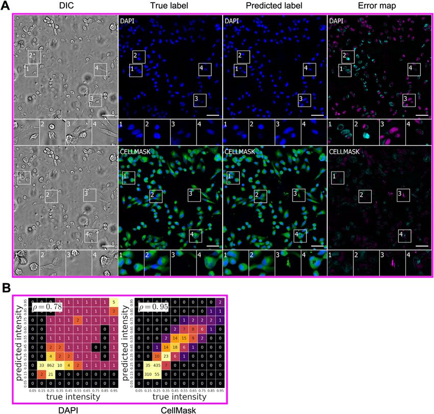
4 Cell 173, 1–12, April 19, 2018

                                                                                                                                                                                                                                           https://doi.org/10.1016/j.cell.2018.03.040
                                                                                                                                                                                                                                           Please cite this article in press as: Christiansen et al., In Silico Labeling: Predicting Fluorescent Labels in Unlabeled Images, Cell (2018),
                                   Table 1. Training Data Types and Configurations
                                                                                      Fluorescent         Fluorescent      Fluorescent                                                                Pixel Width
                                                                                      Label #1 and        Label #2 and     Label #3 and         Training Testing Microscope          Stitched         before/after
                                   Condition                              Transmitted Imaging             Imaging          Imaging              Data     Data    Field per           Image per        Image
                                   Designation Cell Type            Fixed Light       Modality            Modality         Modality             (Wells)  (Wells) Well (mm)           Well (Pixels)b   Processing (nm) Laboratory
                                   A (red)       human motor        yes    bright field   Hoechst         anti-TuJ1        anti-Islet1          22        3         940 3 1,300      1,900 3 2,600 250/500              Rubin
                                                 neuronsa                                 (nuclei)        (neurons)        (motor neurons)
                                                                                          wide field      wide field       wide field
                                   B (yellow)    human motor        yes    phase          DAPI (nuclei)   anti-MAP2        anti-neurofilament 21          4         1,400 3 1,400 4,600 3 4,600 150/300                 Finkbeiner
                                                 neuronsa                  contrast       confocal        (dendrites)      (axons) confocal
                                                                                                          confocal
                                   C (green)     primary rat       no      phase          Hoechst         propidium       –                     72        8         720 3 720        2,400 3 2,400 150/300              Finkbeiner
                                                 cortical cultures         contrast       (nuclei)        iodide (dead
                                                                                          confocal        cells) confocal
                                   D (blue)      primary rat       yes     phase          DAPI (nuclei)   anti-MAP2        anti-neurofilament 2           1         1,400 3 1,400 4,600 3 4,600 150/300                 Finkbeiner
                                                 cortical cultures         contrast       confocal        (dendrites)      (axons) confocal
                                                                                                          confocal
                                   E (violet)    human breast       yes    DIC            DAPI (nuclei)   CellMask         –                    1c        1         1,100 3 1,100 3,500 3 3,500 160/320                 Google
                                                 cancer line                              confocal        (membrane)
                                                                                                          confocal
                                   Color code, which is denoted in parentheses in the first column, refers to the border color in the figures that was added to enhance readability.aDifferentiated from induced pluripotent stem cells.
                                   b
                                     Approximate size after preprocessing.
                                   c
                                     This condition purposely contains only a single well of training data to demonstrate that the model can learn new tasks from very little data through multi-task learning.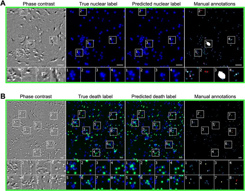
Please cite this article in press as: Christiansen et al., In Silico Labeling: Predicting Fluorescent Labels in Unlabeled Images, Cell (2018),
 https://doi.org/10.1016/j.cell.2018.03.040

Figure 2. Example Images of Unlabeled and Labeled Cells Used to Train the Deep Neural Network
Each row is a typical example of labeled and unlabeled images from the datasets described in Table 1. The first column is the center image from the z-stack of
unlabeled transmitted-light images from which the network makes its predictions. Subsequent columns show fluorescence images of labels that the network will
use to learn correspondences with the unlabeled images and eventually try to predict from unlabeled images. The numbered outsets show magnified views of
subregions of images within a row. The training data are diverse: sourced from two independent laboratories using two different cell types, six fluorescent labels,
and both bright-field and phase-contrast methods to acquire transmitted-light images of unlabeled cells. Scale bars, 40 mm.

                                                                                                                            Cell 173, 1–12, April 19, 2018 5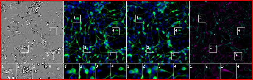
Please cite this article in press as: Christiansen et al., In Silico Labeling: Predicting Fluorescent Labels in Unlabeled Images, Cell (2018),
  https://doi.org/10.1016/j.cell.2018.03.040

                                                                                                      C

           A                               B

Figure 3. Machine-Learning Workflow for Network Development
(A) Example z-stack of transmitted-light images with five colored squares showing the network’s multi-scale input. The squares range in size, increasing from 72
 3 72 pixels to 250 3 250 pixels, and they are all centered on the same fixation point. Each square is cropped out of the transmitted-light image from the z-stack
and input to the network component of the same color in (B).
(B) Simplified network architecture. The network composes six serial sub-networks (towers) and one or more pixel-distribution-valued predictors (heads). The
first five towers process information at one of five spatial scales and then, if needed, rescale to the native spatial scale. The sixth and last tower processes the
information from these towers.
(C) Predicted images at an intermediate stage of image prediction. The network has already predicted pixels to the upper left of its fixation point, but hasn’t yet
predicted pixels for the lower right part of the image. The input and output fixation points are kept in lockstep and are scanned in raster in order to produce the full
predicted images.
See also Figure S6.

lacking DNA). We created heatmaps of true versus predicted                            obtain a quantitative grasp of the network’s behavior, we created
pixel intensities and quantified the correlation. Pearson correla-                    heatmaps and calculated linear fits (Figure 5B). The Pearson
tion (r) values of 0.87 or higher indicated that the network accu-                    r value of 0.85 for propidium iodide indicated a strong linear rela-
rately predicted the extent and level of labeling and that the                        tionship between the true and predicted labels.
predicted pixel intensities reflect the true intensities on a per-                       To understand the network’s ability to recognize cell death and
pixel basis. The network learned features that could be general-                      how it compared to a trained biologist, we had the real and pre-
ized, given that these predictions were made using different cell                     dicted propidium iodide-labeled images annotated, following the
types and image acquisition methods.                                                  same method as for the nuclear labels (Figure 5C). A subset of
   To assess the utility of the per-pixel predictions, we gave a                      the discrepancies between the two annotations in which a biol-
team of biologists real and predicted nuclear label images and                        ogist inspecting the phase contrast images determined that an
asked them to annotate the images with the locations of the                           ‘‘added’’ error is a correct prediction of DNA-free cell debris
cell centers. With annotations on real images as ground truth,                        was reclassified into a new category (Figure S2; STAR Methods).
we used the methodology of Coelho et al. (2009) to classify the                       The network has an empirical precision and recall of 98% at
network’s errors into four categories (Figures 4B and S2A).                           97%, with a 1% chance that two dead cells will be predicted
Under conditions where the amount of cellular debris was high                         to be one dead cell.
(e.g., condition B) or distortions in image quality evident (e.g.,                       To further evaluate the utility and biological significance of the
condition C), the network’s precision and recall drops to the                         quantitative pixel-wise predictions of the network, we wondered
mid-90%. In other cases, the network was nearly perfect, even                         whether network predictions of DAPI/Hoechst labeling could be
with dense cell clumps (e.g., condition D).                                           used to perform morphological analysis of nuclei and accurately
                                                                                      detect and distinguish live cells from dead ones. We showed
Network Predictions of Cell Viability                                                 previously that neurons in vitro tend to die by apoptosis, a pro-
To determine whether transmitted-light images contain sufficient                      grammed cell death process that causes nuclei to shrink and
information to predict whether a cell is alive or dead, we trained                    round up (Arrasate et al., 2004). To perform the analysis, we
the network with images of live cells treated with propidium                          used the transmitted-light images above to make predictions
iodide (PI), a dye that preferentially labels dead cells. We then                     of nuclear labels and then used those collections of pixel predic-
made predictions on withheld images of live cells (Figures 5A                         tions to define nuclear objects and measured their dimensions.
and S1). The network was remarkably accurate, though not as                           We then compared the dimensions of nuclei among cells deter-
much as it was for nuclear prediction. For example, it correctly                      mined to be dead or alive based on propidium iodide labeling.
guessed that an entity (Figure 5A, second magnified outset) is                        We found that the mean size of nuclei of live cells quantified
actually DNA-free cell debris and not a proper cell and picked                        from morphological analysis of pixel-wise predictions was very
out a single dead cell in a mass of live cells (third outset). To                     similar to that measured from actual labels (6.8 ± 1.3 mm vs.

6 Cell 173, 1–12, April 19, 2018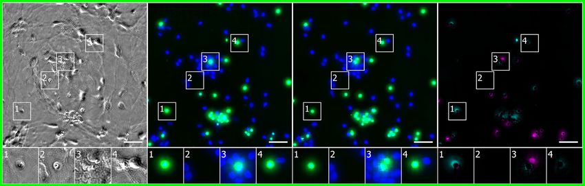
Please cite this article in press as: Christiansen et al., In Silico Labeling: Predicting Fluorescent Labels in Unlabeled Images, Cell (2018),
https://doi.org/10.1016/j.cell.2018.03.040

               A

               B

                                                                                                                           (legend on next page)
                                                                                                             Cell 173, 1–12, April 19, 2018 7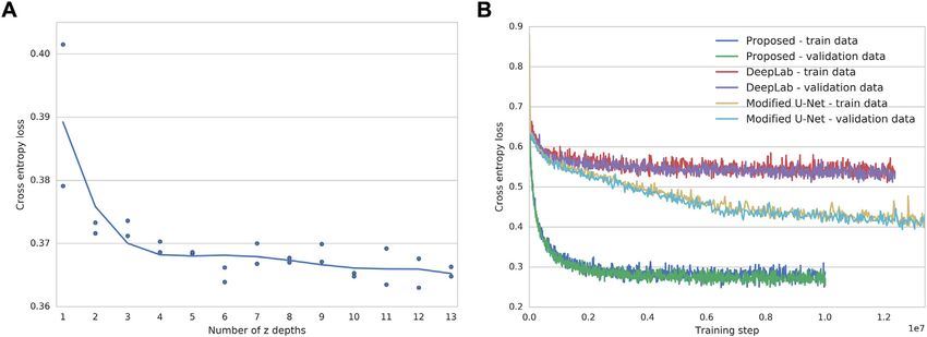
Please cite this article in press as: Christiansen et al., In Silico Labeling: Predicting Fluorescent Labels in Unlabeled Images, Cell (2018),
  https://doi.org/10.1016/j.cell.2018.03.040

7.0 ± 1.4 mm) (Figure S3). Likewise, the nuclear sizes of dead cells                  axon predictions are much better under conditions of low-plating
from predicted labels was very similar to actual measurements                         densities (condition B).
(4.7 ± 1.1 mm versus 4.9 ± 1.0 mm). Importantly, quantitative anal-
ysis of nuclear morphology based on pixel predictions sensitively                     Adapting the Generic Learned Network to New
and accurately identified and distinguished a subset of dead                          Datasets: Transfer Learning
cells from neighboring live cells based on a change in the size                       Does the network require large training datasets to learn to pre-
of their nucleus. The result corroborates the predictions based                       dict new things? Or does the generic model represented by a
on propidium iodide staining and demonstrates the utility of                          trained network enable it to learn new relationships in different
the network to make biologically meaningful quantitative                              datasets more quickly or with less training data than an untrained
morphological measurements based on pixel predictions.                                network? To address these questions, we used transfer learning
                                                                                      to learn a label from a single well, demonstrating that the network
Network Predictions of Cell Type and Subcellular                                      can share learned features across tasks. To further emulate the
Process Type                                                                          experience of a new practitioner adapting this technique to their
We tested the network’s ability to predict which cells were neu-                      research, we chose data using a new label from a different cell
rons in mixed cultures of cells containing neurons, astrocytes,                       type, imaged with a different transmitted-light technology, pro-
and immature dividing cells (Figures 6 and S1). Four biologists                       duced by a laboratory other than those that provided the previ-
independently annotated real and predicted TuJ1 labeling, an                          ous training data. In condition E, differential interference contrast
indication that the cell is a neuron. We compared the annotations                     imaging was used to collect transmitted-light data from unla-
of each biologist (Figure 6) and assessed variability among biol-                     beled cancer cells, and CellMask, a membrane label, was used
ogists by conducting pairwise comparisons of their annotations                        to collect foreground data (Table 1). With only the 1,100 3
on the real labels only.                                                               1,100 mm center of the one training well, regularized by simulta-
   With TuJ1 labels for the condition A culture, the performance                      neously training on conditions A, B, C, and D, the network
of biologists annotating whether an object is a neuron was highly                     learned to predict cell foreground with a Pearson r score of
variable, consistent with the prevailing view that determining cell                   0.95 (Figures S1 and S5). Though that metric was computed
type based on human judgment is difficult. We found humans                            on a single test well, the test images of the well contain 12 million
disagree on whether an object is a neuron 10% of the time,                           pixels each and hundreds of cells. This suggests that the generic
and 2% of the time they disagree on whether an object is                             model represented by the trained network could continue to
one cell or several cells. When a biologist was presented with                        improve its performance with additional training examples, and
true and predicted labels of the same sample, 11%–15% of                              increase the ability and speed with which it learns to perform
the time the type of cell is scored differently from one occasion                     new tasks.
to the next, and 2%–3% of the time the number of cells is scored
differently. Thus, the frequency of inconsistency introduced by                       DISCUSSION
using the predicted labels instead of the true labels is compara-
ble to the frequency of inconsistency between biologists evalu-                       Here, we report a new approach: in silico labeling (ISL). This deep
ating the same true labels.                                                           learning system can predict fluorescent labels from transmitted-
   Given the success of the network in predicting whether a cell is                   light images. The deep neural network we developed could be
a neuron, we wondered whether it also could accurately predict                        trained on unlabeled images to make accurate per pixel predic-
whether a neurite extending from a cell was an axon or a                              tions of the location and intensity of nuclear labeling with DAPI or
dendrite. The task suffers from a global coherence problem                            Hoechst dye and to indicate if cells were dead or alive by predict-
(STAR Methods), and it was also unclear to us a priori whether                        ing propidium iodide labeling. We further show that the network
transmitted-light images contained enough information to distin-                      could be trained to accurately distinguish neurons from other
guish dendrites from axons. Surprisingly, the final network could                     cells in mixed cultures and to predict whether a neurite is an
predict independent dendrite and axon labels (Figures S1 and                          axon or dendrite. These predictions showed a high correlation
S4). It does well in predicting dendrites in conditions of low- (con-                 between the location and intensity of the actual and predicted
dition B) and high- (condition D) plating densities, whereas the                      pixels. They were accurate for live cells, enabling longitudinal

Figure 4. Predictions of Nuclear Labels (DAPI or Hoechst) from Unlabeled Images
(A) Upper-left corner crops of test images from datasets in Table 1; please note that images in all figures are small crops from much larger images and that the
crops were not cherry-picked. The first column is the center transmitted image of the z-stack of images of unlabeled cells used by the network to make its
prediction. The second and third columns are the true and predicted fluorescent labels, respectively. Predicted pixels that are too bright (false positives) are
magenta and those too dim (false negatives) are shown in teal. Condition A, outset 4, and condition B, outset 2, shows false negatives. Condition C, outset 3, and
condition D, outset 1, show false positives. Condition B, outsets 3 and 4, and condition C, outset 2, show a common source of error, where the extent of the
nuclear label is predicted imprecisely. Other outsets show correct predictions, though exact intensity is rarely predicted perfectly. Scale bars, 40 mm.
(B) The heatmaps compare the true fluorescence pixel intensity to the network’s predictions, with inset Pearson r values. The bin width is 0.1 on a scale of zero to
one (STAR Methods). The numbers in the bins are frequency counts per 1,000. Under each heatmap plot is a further categorization of the errors and the per-
centage of time they occurred. Split is when the network mistakes one cell as two or more cells. Merged is when the network mistakes two or more cells as one.
Added is when the network predicts a cell when there is none (i.e., a false positive), and missed is when the network fails to predict a cell when there is one (i.e., a
false negative).
See also Figures S1, S2, S4, S5, and S7.

8 Cell 173, 1–12, April 19, 2018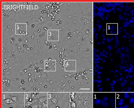
Please cite this article in press as: Christiansen et al., In Silico Labeling: Predicting Fluorescent Labels in Unlabeled Images, Cell (2018),
  https://doi.org/10.1016/j.cell.2018.03.040

            A

            B                                             C

Figure 5. Predictions of Cell Viability from Unlabeled Live Images
(A–C) The trained network was tested for its ability to predict cell death, indicated by labeling with propidium iodide staining shown in green.
(A) Upper-left corner crops of cell death predictions on the datasets from condition C (Table 1). Similarly to Figure 4, the first column is the center phase contrast
image of the z-stack of images of unlabeled cells used by the network to make its prediction. The second and third columns are the true and predicted fluorescent
labels, respectively, shown in green. Predicted pixels that are too bright (false positives) are magenta and those too dim (false negatives) are shown in teal. The
true (Hoechst) and predicted nuclear labels have been added in blue to the true and predicted images for visual context. Outset 1 in (A) shows a misprediction of
the extent of a dead cell, and outset 3 in (A) shows a true positive adjacent to a false positive. The other outsets show correct predictions, though exact intensity is
rarely predicted perfectly. Scale bars, 40 mm.
(B) The heatmap compares the true fluorescence pixel intensity to the network’s predictions, with an inset Pearson r value, on the full condition C test set. The bin
width is 0.1 on a scale of zero to one (STAR Methods). The numbers in the bins are frequency counts per 1,000.
(C) A further categorization of the errors and the percentage of time they occurred. Split is when the network mistakes one cell as two or more cells. Merged is
when the network mistakes two or more cells as one. Added is when the network predicts a cell when there is none (i.e., a false positive), and missed is when the
network fails to predict a cell when there is one (i.e., a false negative).
See also Figures S1–S5 and S7.

fluorescence-like imaging with no additional sample preparation                       bright field z-stacks, and also showed that cell nuclei can be
and minimal impact to cells. Thus, we conclude that unlabeled                         segmented from non-nuclei fluorescent markers. Unfortunately,
images contain substantial information that can be used to train                      the task of predicting fluorescence images from transmitted-
deep neural networks to predict labels in both live and fixed cells                   light images is not well served by typical classification models
that normally require invasive approaches to reveal, or which                         such as Inception (Szegedy et al., 2015a) because they typically
cannot be revealed using current methods.                                             contain spatial reductions that destroy fine detail. In response,
   Deep learning has been applied to achieve useful advances in                       researchers developed specialized models for predicting images
basic segmentation of microscopy images, an initial step in im-                       from images, including DeepLab (Chen et al., 2015) and U-Net
age analysis to distinguish foreground from background (Chen                          (Ronneberger et al., 2015). However, we had limited success
and Chefd’hotel, 2014; Dong et al., 2015; Mao et al., 2015; Ron-                      with these networks (Figure S6; STAR Methods) and, thus,
neberger et al., 2015; Van Valen et al., 2016; Xu et al., 2016), and                  created a new one.
on segmented images of morphologically simple cells to classify                          Our deep neural network comprises repeated modules, such
cell shape (Zhong et al., 2012) and predict mitotic state (Held                       as the reported Inception network, but the modules differ in
et al., 2010) and cell lineage (Buggenthin et al., 2017). (Long                       important ways (STAR Methods). Inspired by U-Net (Ronne-
et al., 2010) applied deep learning methods to unlabeled and                          berger et al., 2015), it is constructed so that fine-grain informa-
unsegmented images of low-density cultures with mixtures of                           tion can flow from the input to the output without being degraded
three cell types and trained a network to classify cell types. (Sa-                   by locality destroying transformations. It is multi-scale to provide
danandan et al., 2017) used deep learning to segment cells from                       context, and it preserves approximate translation invariance by

                                                                                                                                Cell 173, 1–12, April 19, 2018 9
Please cite this article in press as: Christiansen et al., In Silico Labeling: Predicting Fluorescent Labels in Unlabeled Images, Cell (2018),
https://doi.org/10.1016/j.cell.2018.03.040
A
B C
Figure 6. Predictions of Cell Type from Unlabeled Images
(A–C) The network was tested for its ability to predict from unlabeled images which cells are neurons. The neurons come from cultures of induced pluripotent stem
cells differentiated toward the motor neuron lineage but which contain mixtures of neurons, astrocytes, and immature dividing cells.
(A) Upper-left corner crops of neuron label (TuJ1) predictions, shown in green, on the condition A data (Table 1). The unlabeled image that is the basis for the
prediction and the images of the true and predicted fluorescent labels are organized similarly to Figure 4. Predicted pixels that are too bright (false positives) are
magenta and those too dim (false negatives) are shown in teal. The true and predicted nuclear (Hoechst) labels have been added in blue to the true and predicted
images for visual context. Outset 3 in (A) shows a false positive: a cell with a neuronal morphology that was not TuJ1 positive. The other outsets show correct
predictions, though exact intensity is rarely predicted perfectly. Scale bars, 40 mm.
(B) The heatmap compares the true fluorescence pixel intensity to the network’s predictions, with inset Pearson r values, on the full condition A test set. The bin
width is 0.1 on a scale of zero to one (STAR Methods). The numbers in the bins are frequency counts per 1,000.
(C) A further categorization of the errors and the percentage of time they occurred. The error categories of split, merged, added, and missed are the same as in
Figure 4. An additional ‘‘human vs. human’’ column shows the expected disagreement between expert humans predicting which cells were neurons from the true
fluorescence image, treating a random expert’s annotations as ground truth.
See also Figures S1, S4, S5, and S7.
avoiding zero-padding in the convolutions (STAR Methods), sify the biological state of the cell, which we validated with inde-
which minimizes boundary effects in the predicted images. pendent direct measurements. This shows that labels predicted
Finally, it is specified as the repeated application of a single from a deep learning network may be useful for accurately
parameterized module, which simplifies the design space inferring measurements of the underlying biological structures,
and makes it tractable to automatically search over network concentrations, etc, . . . that they are trained to represent. Lastly,
architectures. the fact that successful predictions were made under differing
We also gained insights into the strengths, limitations, and conditions suggests that the approach is robust and may have
potential applications of deep learning for biologists. The accu- wide applications.
rate predictions at a per-pixel level indicate that direct corre- ISL may offer, at negligible additional cost, a computational
spondences exist between unlabeled images and at least approach to reliably predict more labels than would be feasible
some fluorescent labels. The high correlation coefficients for to collect otherwise from an unlabeled image of a single sample.
several labels indicate that the unlabeled images contain the Also, because ISL works on unlabeled images of live cells,
information for a deep neural network to accurately predict the repeated predictions can be made for the same cell over time
location and intensity of the fluorescent label. Importantly, we without invasive labeling or other perturbations. Many-label
were able to show, in at least one case (Figure S3), that the pre- (multi-plexed) methods exist that partially overcome the barrier
dicted label could be used to accurately quantify the dimensions imposed by spectral overlap, notably via iterative labeling or hy-
of the cellular structure it represented and thereby correctly clas- perspectral imaging. However, the iterative methods are lethal to
10 Cell 173, 1–12, April 19, 2018Please cite this article in press as: Christiansen et al., In Silico Labeling: Predicting Fluorescent Labels in Unlabeled Images, Cell (2018),
https://doi.org/10.1016/j.cell.2018.03.040
cells, and the hyperspectral methods require a specialized setup d QUANTIFICATION AND STATISTICAL ANALYSES
and are limited by the distinctiveness of the fluorophores’ B Statistical calculations
spectra. B Manual identification of network errors
That successful predictions could be made by a singly trained B Noise and predictions near the noise floor
network on data from three laboratories suggests that the B Live versus dead cell nuclear size
learned features are robust and generalizable. We showed that d DATA AND SOFTWARE AVAILABILITY
the trained network could learn a new fluorescent label from a
very limited set of labeled data collected with a different SUPPLEMENTAL INFORMATION
microscopy method. This suggests that the trained network
Supplemental Information includes seven figures, one table, and one data file and
exhibited transfer learning. In transfer learning, the more a model
can be found with this article online at https://doi.org/10.1016/j.cell.2018.03.040.
has learned, the less data it needs to learn a new similar task. It
applies previous lessons to new tasks. Thus, this network could ACKNOWLEDGMENTS
improve with additional training data and might make accurate
predictions on a broader set of data than we measured. We thank Lance Davidow for technical assistance; Mariya Barch for advice
Nevertheless, we encountered clear limitations of the current and helpful discussions about the manuscript; Marija Pavlovic for preparing
network’s predictive ability. With supervised ML, the quality of the condition E samples; Francesca Rapino and Max Friesen for providing
additional cell types not used in this manuscript; Michelle Dimon for helpful
predictions is limited by the information contained in the input
advice; Charina Choi, Amy Chou, Youness Bennani-Smires, Gary Howard,
data. For example, the network was less successful in identi- and Kelley Nelson for editorial assistance; and Michael Frumkin and Kevin
fying axons in high-density cultures. Although the network P. Murphy for supporting the project.
identified neurons in mixed cultures well, it was unsuccessful
in predicting the motor neuron subtype (Figure S7). The accu- AUTHOR CONTRIBUTIONS
racy will be limited if there is little or no correspondence
between pixels in the unlabeled image and those in the fluores- Conceptualization, E.M.C., S.J.Y., D.M.A., A.J., G.S., S.L., M.B., L.L.R., P.N.,
and S.F.; Methodology, E.M.C., S.J.Y., D.M.A., A.J., G.S., S.L., E.M., K.S.,
cently labeled one, if the quality of labeling is severely affected
A.E., M.B., and S.F.; Software, E.M.C., S.J.Y., W.F., R.P., and A.E.; Validation,
due to contributions from non-specific binding or variability, or
E.M.C., S.J.Y., W.F., and A.E.; Formal Analysis, E.M.C., S.J.Y., A.J., G.S., S.L.,
if the data are insufficient. We found from error analysis that the W.F., R.P., and A.E.; Investigation, E.M.C., S.J.Y., D.M.A., E.M., A.O., K.S.,
performance of the network depended on the amount of infor- A.K.L., P.G., and W.F.; Resources, E.M.C., A.J., G.S., S.L., A.K.L., L.L.R.,
mation in the unlabeled images, as measured by the number of P.N., and S.F.; Data Curation, E.M.C., S.J.Y., D.M.A., A.J., G.S., S.L., and
images in the z-stack (Figure S6), though we suspect transfer E.M.; Writing – Original Draft, E.M.C., S.J.Y., A.O., W.F., R.P., and S.F.;
learning and better imaging protocols may reduce the need Writing – Review & Editing, E.M.C., S.J.Y., D.M.A., A.J., G.S., S.L., W.F.,
A.E., L.L.R., P.N., and S.F.; Visualization, E.M.C. and S.J.Y.; Supervision,
for a z-stack. One challenge is the empirical quality of deep
A.J., G.S., M.B., L.L.R., P.N., and S.F.; Project Administration, E.M.C., P.N.,
learning approaches. Network architecture and training ap- and S.F.; and Funding Acquisition, S.L., P.N., and S.F.
proaches can be optimized to perform at impressive levels,
but it can be difficult to determine general principles of how DECLARATION OF INTERESTS
the network made or failed to make predictions that might
guide future improvements. This will be an important area for Eric Christiansen, Samuel J. Yang, D. Michael Ando, Ryan Poplin, Marc
future research. Berndl, and Philip Nelson are employees of Google, which may benefit finan-
cially from increased scientific use of cloud computing. All other authors
declare no competing interests.
STAR+METHODS
Received: August 14, 2017
Detailed methods are provided in the online version of this paper Revised: December 13, 2017
Accepted: March 15, 2018
and include the following:
Published: April 12, 2018
d KEY RESOURCES TABLE
SUPPORTING CITATIONS
d CONTACT FOR REAGENT AND RESOURCE SHARING
d EXPERIMENTAL MODEL AND SUBJECT DETAILS The following reference appears in the Supplemental Information: Goodfellow
B Cell preparation et al. (2016).
d METHOD DETAILS
B Fluorescent labeling REFERENCES
B Imaging
B Data preparation Abadi, M., Agarwal, A., Barham, P., Brevdo, E., Chen, Z., Citro, C., Corrado,
G., Davis, A., Dean, J., Devin, M., et al. (2015). TensorFlow: large-scale
B Machine learning
machine learning on heterogeneous distributed systems. arXiv, ar-
B Performance dependence on z stack size Xiv:1603.04467v2, https://arxiv.org/abs/1603.04467.
B Limitations
Arrasate, M., Mitra, S., Schweitzer, E.S., Segal, M.R., and Finkbeiner, S.
B Global coherence (2004). Inclusion body formation reduces levels of mutant huntingtin and the
B Comparison to other deep neural networks risk of neuronal death. Nature 431, 805–810.
B A note on 3D prediction Buggenthin, F., Buettner, F., Hoppe, P.S., Endele, M., Kroiss, M., Strasser, M.,
B Image processing in figures Schwarzfischer, M., Loeffler, D., Kokkaliaris, K.D., Hilsenbeck, O., et al. (2017).
Cell 173, 1–12, April 19, 2018 11Please cite this article in press as: Christiansen et al., In Silico Labeling: Predicting Fluorescent Labels in Unlabeled Images, Cell (2018),
https://doi.org/10.1016/j.cell.2018.03.040
Prospective identification of hematopoietic lineage choice by deep learning. Pagliuca, F.W., Millman, J.R., Gürtler, M., Segel, M., Van Dervort, A., Ryu, J.H.,
Nat. Methods 14, 403–406. Peterson, Q.P., Greiner, D., and Melton, D.A. (2014). Generation of functional
Burkhardt, M.F., Martinez, F.J., Wright, S., Ramos, C., Volfson, D., Mason, M., human pancreatic b cells in vitro. Cell 159, 428–439.
Garnes, J., Dang, V., Lievers, J., Shoukat-Mumtaz, U., et al. (2013). A cellular Ramsundar, B., Kearnes, S., Riley, P., Webster, D., Konerding, D., and Pande,
model for sporadic ALS using patient-derived induced pluripotent stem cells. V. (2015). Massively multitask networks for drug discovery. ar-
Mol. Cell. Neurosci. 56, 355–364. Xiv:1502.02072v1, https://arxiv.org/abs/1502.02072.
Carpenter, A.E., Jones, T.R., Lamprecht, M.R., Clarke, C., Kang, I.H., Friman, Rigamonti, A., Repetti, G.G., Sun, C., Price, F.D., Reny, D.C., Rapino, F., Wei-
O., Guertin, D.A., Chang, J.H., Lindquist, R.A., Moffat, J., et al. (2006). singer, K., Benkler, C., Peterson, Q.P., Davidow, L.S., et al. (2016). Large-scale
CellProfiler: image analysis software for identifying and quantifying cell pheno- production of mature neurons from human pluripotent stem cells in a three-
types. Genome Biol. 7, R100. dimensional suspension culture system. Stem Cell Reports 6, 993–1008.
Chen, T., and Chefd’hotel, C. (2014). Deep learning based automatic immune Ronneberger, O., Fischer, P., and Brox, T. (2015). U-net: convolutional
cell detection for immunohistochemistry images. In Machine Learning in networks for biomedical image segmentation. In International Conference on
Medical Imaging, G. Wu, D. Zhang, and L. Zhou, eds. (Springer International Medical Image Computing and Computer-Assisted Intervention, N. Navab,
Publishing), pp. 17–24. J. Hornegger, W.M. Wells, and A.F. Frangi, eds. (Springer), pp. 234–241.
Chen, L.-C., Papandreou, G., Kokkinos, I., Murphy, K., and Yuille, A.L. (2015). Sadanandan, S.K., Ranefall, P., Le Guyader, S., and Wählby, C. (2017). Auto-
Semantic image segmentation with deep convolutional nets and fully mated training of deep convolutional neural networks for cell segmentation.
connected CRFs. arXiv:1412.7062v4, https://arxiv.org/abs/1412.7062 . Sci. Rep. 7, 7860.
Coelho, L.P., Shariff, A., and Murphy, R.F. (2009). Nuclear segmentation in Schroff, F., Kalenichenko, D., and Philbin, J. (2015). Facenet: A unified embed-
microscope cell images: a hand-segmented dataset and comparison of algo- ding for face recognition and clustering.arXiv:1503.03832v3, https://arxiv.org/
rithms. Proc. IEEE Int. Symp. Biomed. Imaging 5193098, 518–521. abs/1503.03832.
Dong, B., Shao, L., Costa, M.D., Bandmann, O., and Frangi, A.F. (2015). Deep Silver, D., Huang, A., Maddison, C.J., Guez, A., Sifre, L., van den Driessche, G.,
learning for automatic cell detection in wide-field microscopy zebrafish Schrittwieser, J., Antonoglou, I., Panneershelvam, V., Lanctot, M., et al. (2016).
images. In 2015 IEEE 12th International Symposium on Biomedical Imaging Mastering the game of go with deep neural networks and tree search. Nature
(ISBI), 772–776. 529, 484–489.
Du, Z.-W., Chen, H., Liu, H., Lu, J., Qian, K., Huang, C.-L., Zhong, X., Fan, F., Snoek, J., Larochelle, H., and Adams, R.P. (2012). P. In Advances in Neural
and Zhang, S.-C. (2015). Generation and expansion of highly pure motor Information Processing Systems 25, Pereira., C.J.C. Burges, L. Bottou, and
neuron progenitors from human pluripotent stem cells. Nat. Commun. 6, 6626. K.Q. Weinberger, eds. (Curran Associates), pp. 2951–2959.
Duchi, J., Hazan, E., and Singer, Y. (2011). Adaptive subgradient methods for Szegedy, C., Liu, W., Jia, Y., Sermanet, P., Reed, S., Anguelov, D., Erhan, D.,
online learning and stochastic optimization. J. Mach. Learn. Res. 12, Vanhoucke, V., and Rabinovich, A. (2015a). Going deeper with convolutions.
2121–2159. arXiv:1409.4842v1, https://arxiv.org/abs/1409.4842.
Dumoulin, V., and Visin, F. (2016). A guide to convolution arithmetic for deep Szegedy, C., Vanhoucke, V., Ioffe, S., Shlens, J., and Wojna, Z. (2015b).
learning. arXiv:1603.07285v2, https://arxiv.org/abs/1603.07285. Rethinking the inception architecture for computer vision. arXiv:
1512.00567v3, https://arxiv.org/abs/1512.00567.
Farabet, C., Couprie, C., Najman, L., and Lecun, Y. (2013). Learning hierarchi-
Szegedy, C., Ioffe, S., and Vanhoucke, V. (2016). Inception-v4, Inception-
cal features for scene labeling. IEEE Trans. Pattern Anal. Mach. Intell. 35,
ResNet and the impact of residual connections on learning. arXiv:
1915–1929.
1602.07261v2, https://arxiv.org/abs/1602.07261.
Finkbeiner, S., Frumkin, M., and Kassner, P.D. (2015). Cell-based screening:
van den Oord, A., Kalchbrenner, N., and Kavukcuoglu, K. (2016). Pixel recur-
extracting meaning from complex data. Neuron 86, 160–174.
rent neural networks. arXiv:1601.06759v3, https://arxiv.org/abs/1601.06759.
Golovin, D., Solnik, B., Moitra, S., Kochanski, G., Karro, J., and Sculley, D.
van der Walt, S., Colbert, S.C., and Varoquaux, G. (2011). The NumPy array: a
(2017). Google Vizier: a service for black-box optimization. In Proceedings of
structure for efficient numerical computation. Comput. Sci. Eng. 13, 22–30.
the 23rd ACM SIGKDD International Conference on Knowledge Discovery
and Data Mining (ACM), pp. 1487–1495. Van Valen, D.A., Kudo, T., Lane, K.M., Macklin, D.N., Quach, N.T., DeFelice,
M.M., Maayan, I., Tanouchi, Y., Ashley, E.A., and Covert, M.W. (2016). Deep
Goodfellow, I.J., Pouget-Abadie, J., Mirza, M., Xu, B., Warde-Farley, D., Ozair,
learning automates the quantitative analysis of individual cells in live-cell imag-
S., Courville, A., and Bengio, Y. (2014). Generative adversarial nets. ar-
ing experiments. PLoS Comput. Biol. 12, e1005177.
Xiv:1406.2661v1, https://arxiv.org/abs/1406.2661.
Waskom, M., Botvinnik, O., Drewokane, Hobson, P., Halchenko, Y., Lukaus-
Goodfellow, I., Bengio, Y., and Courville, A. (2016). Deep Learning (MIT Press).
kas, S., Warmenhoven, J., Cole, J.B., Hoyer, S., Vanderplas, J., et al. (2016).
He, K., Zhang, X., Ren, S., and Sun, J. (2016). Identity mappings in deep resid- seaborn: v0.7.0.
ual networks. arXiv:1603.05027v3, https://arxiv.org/abs/1603.05027.
Wikipedia (2017a). Softmax function. https://en.wikipedia.org/w/index.php?
Held, M., Schmitz, M.H.A., Fischer, B., Walter, T., Neumann, B., Olma, M.H., title=Softmax_function&oldid=829752166.
Peter, M., Ellenberg, J., and Gerlich, D.W. (2010). CellCognition: time-resolved
Wikipedia (2017b). Unbiased estimation of standard deviation. https://en.
phenotype annotation in high-throughput live cell imaging. Nat. Methods 7,
wikipedia.org/w/index.php?
747–754.
title=Unbiased_estimation_of_standard_deviation&oldid=823365997.
Jones, E., Oliphant, T., and Peterson, P. (2001). SciPy: open source scientific Xu, Y., Li, Y., Liu, M., Wang, Y., Lai, M., and I.-Chao Chang, E. (2016). Gland
tools for Python. instance segmentation by deep multichannel side supervision. arXiv:
Kingma, D., and Ba, J. (2014). Adam: A method for stochastic optimization. 1607.03222v2, https://arxiv.org/abs/1607.03222.
arXiv:1412.6980v9, https://arxiv.org/abs/1412.6980. Zeiler, M.D., Krishnan, D., Taylor, G.W., and Fergus, R. (2010). Deconvolutional
Long, X., Cleveland, W.L., and Yao, Y.L. (2010). Multiclass detection of cells in networks. In Computer Vision and Pattern Recognition (CVPR), 2010 IEEE
multicontrast composite images. Comput. Biol. Med. 40, 168–178. Conference on (IEEE), pp. 2528–2535.
Mao, Y., Yin, Z., and Schober, J.M. (2015). Iteratively training classifiers for Zhong, Q., Busetto, A.G., Fededa, J.P., Buhmann, J.M., and Gerlich, D.W.
circulating tumor cell detection. In 2015 IEEE 12th International Symposium (2012). Unsupervised modeling of cell morphology dynamics for time-lapse
on Biomedical Imaging (ISBI) (IEEE), pp. 190–194. microscopy. Nat. Methods 9, 711–713.
12 Cell 173, 1–12, April 19, 2018Please cite this article in press as: Christiansen et al., In Silico Labeling: Predicting Fluorescent Labels in Unlabeled Images, Cell (2018),
https://doi.org/10.1016/j.cell.2018.03.040
STAR+METHODS
KEY RESOURCES TABLE
REAGENT or RESOURCE SOURCE IDENTIFIER
Antibodies
rabbit a-Islet Abcam 109517
mouse a-Tuj Biolegend 801202
chicken a-MAP2 Abcam 5392
rabbit a-NF-H Encor RPCA-NF-H
Goat anti rabbit IgG Alexa 488 Invitrogen A-11034
Goat anti mouse IgG Alexa 546 Invitrogen A-11003
Biological Samples
Long-Evans outbred rats Charles River Strain Code # 006
Chemicals, Peptides, and Recombinant Proteins
DMEM-F12 Life Technologies 11330057
Neurobasal Life Technologies 21103049
Knockout Serum Replacement Life Technologies 10828028
NEAA EMD Millipore TMS-001-C
Pen-Strep Life Technologies 15140-163
Glutamax Life Technologies 35050-061
D-Glucose Solution Sigma G8270
N2 Supplement Life Technologies 17502-048
B27 Supplement Life Technologies 17504-044
Ascorbic Acid Sigma A4403
DNase Worthington LK003172
EBSS Life Technologies 24010043
BDNF R&D Systems 248-BD-01M
GDNF R&D Systems 512-gf-010
CTNF R&D Systems 557-NT
Poly-Ornithine Sigma P3655
Laminin Sigma L2020
DPBS Life Technologies 14190-235
Neurobasal Life Technologies 21103049
2-Mercaptoethanol Life Technologies 21985023
mTESR1 StemCell Technologies 5850
Accutase StemCell Technologies 7920
Smoothened Agonist 1.3 EMD Biosciences 566660
LDN StemGent 04-0074-02
SB431542 R&D Systems 1614
Retinoic Acid Sigma R2625
Paraformaldehyde Electron Microscopy Sciences 15710
Bovine Serum Albumin (BSA) VWR RLBSA
Fetal Bovine Serum (FBS) Sigma F2442
Hoescht 33342 Sigma B2261
Modified Eagle Medium Dulbecco n/a
Fetal bovine sera n/a n/a
CellMask Deep Red membrane stain Life Technologies C10046
PBS Life Technologies 28906
(Continued on next page)
Cell 173, 1–12.e1–e11, April 19, 2018 e1Please cite this article in press as: Christiansen et al., In Silico Labeling: Predicting Fluorescent Labels in Unlabeled Images, Cell (2018),
https://doi.org/10.1016/j.cell.2018.03.040
Continued
REAGENT or RESOURCE SOURCE IDENTIFIER
Prolong Diamond with DAPI Thermo Fisher P36962
ReadyProbes Cell Viability (Blue/Green) Thermo Fisher Scientific R37609
Na2SO4 Sigma 239313-500
K2SO4 Sigma P9458-1kg
MgCl2 Sigma M2393-500G
CaCl2 Sigma C5080-500G
HEPES Calbiochem 391338
Glucose Macron fine chemicals 4912-12
Phenol red Sigma P-0290
NaOH Sigma S588-500G
Kynurenic acid (1 mM final) Sigma K3375-5G
Papain (100 U) Worthington Biochemical LS003126
Trypsin inhibitor Sigma T9253-5G
Opti-MEM (Thermo Fisher Scientific Thermo Fisher Scientific 31985070
100X GlutaMAX Thermo Fisher Scientific 35050061
Pen/Strep Thermo Fisher Scientific 15140122
B27 supplement Thermo Fisher Scientific 17504044
Experimental Models: Cell Lines
1016A-WT iPSC Pagliuca et al., 2014 hiPSC-2
MDA-MB-231 ATCC HTB-26
Healthy iPSC line differentiated into motor neurons Yamanaka lab KW4
Software and Algorithms
Google Cloud Dataflow Google https://cloud.google.com/dataflow
TensorFlow Abadi et al., 2015 https://www.tensorflow.org
Google Hypertune Golovin et al., 2017 https://cloud.google.com/ml-engine/
docs/hyperparameter-tuning-overview
SciPy Jones et al., 2001 https://www.scipy.org
seaborn Waskom et al., 2016 https://seaborn.pydata.org
CellProfiler Carpenter et al., 2006 http://cellprofiler.org/
Code and data for this paper This paper https://github.com/google/in-silico-labeling
Other
40 mM Cell Strainer Corning (Falcon) 352340
15 mL Tubes Corning/Falcon 352096
50 mL Tubes Corning/Falcon 352070
96 well mClear Plate CELLSTAR Greiner Bio-One 82050-748
CONTACT FOR REAGENT AND RESOURCE SHARING
Further information and requests for resources and reagents should be directed to and will be fulfilled by the Lead Contact, Eric
Christiansen (ericmc@google.com).
EXPERIMENTAL MODEL AND SUBJECT DETAILS
Cell preparation
Condition A
The human iPSC line 1016A was differentiated as described in (Rigamonti et al., 2016). Briefly, iPSCs were grown to near confluency
in adherent culture in mTesr media (StemCell Technologies) before being dissociated to single cells using Accutase (cat# 07920,
StemCell Technologies). Single cells were seeded into a spinning bioreactor (Corning, 55 rpm) at 1x10⁶ cells/mL in mTesr with
Rock Inhibitor (10 mM) and kept in 3D suspension culture for the duration of differentiation. The next day (day 1), dual SMAD inhibitors
e2 Cell 173, 1–12.e1–e11, April 19, 2018You can also read