Working Paper Series Global financial markets and oil price shocks in real time
←
→
Page content transcription
If your browser does not render page correctly, please read the page content below

Working Paper Series
          Fabrizio Venditti, Giovanni Veronese   Global financial markets and
                                                 oil price shocks in real time

                                                   No 2472 / September 2020

Disclaimer: This paper should not be reported as representing the views of the European Central Bank
(ECB). The views expressed are those of the authors and do not necessarily reflect those of the ECB.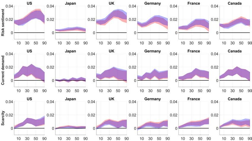
Abstract

           The role that the price of oil plays in economic analysis in central banks as well as in
       financial markets has evolved over time. Oil is not seen anymore just as a input to
       production but also as a barometer of global economic activity as well as a financial
       asset. A high frequency structural decomposition of the price of oil can therefore
       inform on the state of the global business cycle as well as on global financial market
       sentiment. In this paper we develop a method to identify structural sources of oil
       price fluctuations at the daily frequency and in real time. The identification strategy
       blends sign, narrative restrictions and instrumental variable techniques. By using
       data on asset prices, oil production and global economic activity we account for the
       double nature of oil: a financial asset as well as a physical commodity. The model
       offers novel insights on the relationship between the price of oil and asset prices. We
       also illustrate how the model could have been used in real time to interpret oil price
       movements in periods of high geopolitical tensions between the US and Iran and to
       read the drop of crude prices due to fears related to the Corona virus.

           JEL classification: Q43, C32, E32, C53
       Keywords: Oil prices, VAR, Proxy-SVAR, Sign Restrictions.

ECB Working Paper Series No 2472 / September 2020                                                     1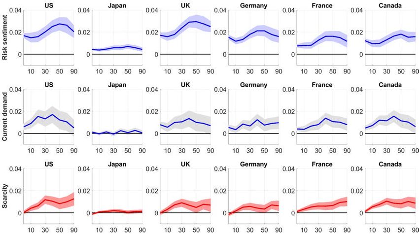
Non Technical Summary

 Disentangling the structural drivers of the price of oil is crucial both for policy makers as well
 as for market participants. First, oil is an important input into economic production and
 sustained (supply driven) price increases can throw the global economy into recession.
 Second, oil prices impact directly inflation and consumer spending through energy prices, as
 oil prices are passed on (one to one) to gasoline prices within a week. Third, commodity
 prices, move strongly in sync with the global business cycle. Finally, in recent years, oil has
 become an important financial asset. However, the models that are most frequently used for
 assessing the structural drivers of oil prices typically rely on low-frequency variables that are
 only available with a substantial delay. As a result, these models typically paint an outdated
 picture of the state of the economy, and are not particularly useful when more timely
 information is needed.

 In this paper we develop a new method for decomposing the price of oil into its structural
 drivers in real time at the daily frequency, exploiting the relationship between oil prices and
 global financial markets. Using a daily structural Vector Autoregression (VAR), in which we
 jointly model spot and futures oil prices as well as stock prices, we decompose the price of oil
 in three structural shocks. The first shock is a forward looking demand shock, which captures
 the impact on the oil price of changes in expectations about future economic activity. We
 label this shock, risk sentiment shock, as it embodies unexpected changes in the risk
 sentiment of market participants on the outlook of global activity. The second shock is an
 unexpected change in the current state of the business cycle and, as a consequence, in
 commodities demand more broadly. The third shock is a supply shock, which captures but
 current and expected changes in oil supply.

 We use the model to analyze fluctuations in the oil price and their relationship with global
 financial markets (equities, bonds, inflation swaps and currencies) using data between June
 2007 and February 2020. We find that risk sentiment shocks induce a parallel shift of the oil
 futures curve: a one percent increase in the price of oil due to a risk sentiment shock is
 associated with a rise of about one percent in 12 months ahead futures prices. More generally,
 a positive risk sentiment shock raises global stock prices, reduces volatility, raises interest
 rates as well as inflation expectations and leads to a depreciation of typical safe haven
 currencies, namely the USD, the Japanese yen and the Swiss franc. The effects of current
 demand shocks are qualitatively similar to, but quantitatively very different from, those of

ECB Working Paper Series No 2472 / September 2020                                                     2
risk sentiment shocks. They have very small effects on oil prices futures and, as consequence,
 a strong negative impact on the slope of the futures curve. The response of financial asset
 prices to a positive current demand shock is consistent with an improved macroeconomic
 environment. Stock prices and bond yields rise, while volatility falls. Safe haven currencies
 depreciate, but less than in response to risk sentiment shocks. Importantly long-term market
 based inflation expectations do not respond to these shocks, suggesting that the information
 content of risk sentiment and current demand shocks is indeed different. Finally, an increase
 in the price of oil due to a negative scarcity shocks is associated with a fall in risky asset
 prices, an increase in financial volatility and a depreciation of the dollar. In general, however,
 the effect of scarcity shocks on financial asset prices is quantitatively very limited. Long-term
 inflation expectations constitute an important exception, as they respond significantly, albeit
 with a delay, also to scarcity shocks, suggesting that the latter might shift inflation risk
 premia.

 As a final exercise, we illustrate how the model could have been used in real time to analyze
 the structural drivers of oil price developments between January and February 2020. This
 period was characterized first by a marked increase in crude prices, as geopolitical tensions
 between the US and Iran spiked following the killing of the Iranian general Soleimani by a
 US drone, then by a collapse of oil (and financial) markets due to the Corona virus. Our
 model neatly distinguishes the main drivers of the price of oil around these episodes,
 attributing the rise in early January to scarcity shocks and the bulk of the Corona virus related
 collapse to a combination of risk sentiment and current demand shocks.

ECB Working Paper Series No 2472 / September 2020                                                     3
As I said, we are monitoring the data. [...] The market sends a signal that it expects the rate
 hike to be much later than what we have said. It’s too early to have the discussion because we are
 still (in the process of ) understanding the nature of the shock.
                                                                                       B. Cœuré.a
    a
     Interview with Mr Benoı̂t Cœuré, Member of the Executive Board of the European Central Bank,
 and Bloomberg TV, conducted by Ms Francine Lacqua on 25 January 2019. Available at https:
 //www.bis.org/review/r190128a.htm

1       Introduction
Every day policy makers inspect the behaviour of financial markets and macroeconomic
data releases to learn about the structural shocks that move asset prices and macroeconomic
aggregates. The task is not trivial. Macroeconomic data are only available with a significant
lag and are subject to non-negligible revisions. Financial asset prices, on the other hand, are
available in real time but are only imperfectly related to the macroeconomic variables that
policy makers ultimately care about, namely output and inflation. The tension between
using information that is timely but noisy and information that is accurate but lagging is
the key challenge for economic analysis in real time. Although “the economy does not cease
to exist in between observations” (Bartlett, 1946) understanding the nature of the shocks
driving its current state is inherently difficult. The problem that the publication lag poses
for real time economic analysis has been extensively analyzed in the context of forecasting
(Banbura, Giannone, Modugno, and Reichlin, 2013). Yet, exactly the same problem arises
when trying to understand in real time the nature of the structural shocks that shape
macroeconomic developments. The models that are most frequently used for this purpose,
i.e. Structural Vector Autoregressions, typically rely on low-frequency variables that are
only available with a substantial delay. As a result, the decomposition of economic data
into structural shocks that these models provide typically paints an outdated picture of the
state of the economy.
    The price of oil plays, in this context, a crucial role for four reasons. First, oil is an
important input into economic production and a sustained (supply driven) increase in its
price can potentially throw the global economy into a recession (Kanzig, 2018). Second, the
price of oil impacts directly inflation and consumer spending through energy prices, as oil
prices are passed on (one to one) to gasoline prices within a week (Venditti, 2013). Third,

ECB Working Paper Series No 2472 / September 2020                                                  4
the price of oil, and more generally commodity prices, are strongly correlated with the
global business cycle, and provide a timely gauge of the state of the economy (Delle Chiaie,
Ferrara, and Giannone, 2017; Sockin and Xiong, 2015); developments in the oil market also
play an important role in how business news ultimately impact financial markets, and can
therefore help in measuring the overall state of the economy (Bybee, Kelly, Manela, and
Xiu, 2020). Finally, in recent years, oil has become an important financial asset, which can
be traded either as a risky asset, given its positive correlation with the business cycle, or to
hedge against geopolitical risk that involves oil producing countries.
    Since Kilian (2009) opened the box of structural identification in global oil markets,
distinguishing the relative role of demand and supply in driving the price of oil has been at
the center of a lively debate in the literature. Such a distinction has far reaching policy
implications, especially for monetary policy makers. The source of the shock matters for
its transmission to inflation, as well as to inflation expectations at different horizons, a
key piece of information for central banks and especially for those following an inflation
targeting strategy. While demand shocks call for determined policy action, supply shocks
usually require a smoother and more protracted policy response (Schnabel, 2020). A real
time structural decomposition of the price of oil would, therefore, allow policy makers and
financial market observers to gauge the nature of the shocks that hit the real economy and
that shape the relationship between oil and financial markets. However structural models
of the oil market, like those put forward by Kilian and Murphy (2014), Caldara, Cavallo,
and Iacoviello (2019), Baumeister and Hamilton (2019), are only available at the monthly
frequency and rely on data that are published with between two to three months delay
with respect to the reference period.
    The main motivation of this paper, and its main contribution to the literature, is to fill
this gap by providing a method for decomposing the price of oil into its structural drivers
in real time. The core of the method is a daily structural VAR that jointly models the price
of oil, stock prices and the price of 12 months ahead oil futures. In constructing this model,
one issue that we face is which measure of equity prices to use. The few papers that look
at the high frequency correlation between oil prices and the stock market typically look at
a broad market index for the US, for instance the S&P 500 index. This, however, has a
number of shortcomings. The S&P 500 index is a float-adjusted index weighted by market

ECB Working Paper Series No 2472 / September 2020                                              5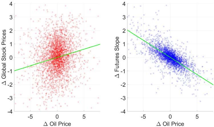
capitalization and a quick look at the weights used in the index reveals that the largest
companies operate in sectors (Information Technology or Financial Services) in which the
direct impact of oil price fluctuations is negligible. We therefore take a different approach
and rely on a particular sector to extract high frequency information on structural shocks,
namely the airline sector. We pick this sector because of the direct relevance that energy
costs have for the profitability of transport companies. We can, therefore, confidently
assume that a negative oil supply shock will raise operating costs for airlines, denting their
profitability and weakening their equity prices. Implicitly, we are also making a second
identification assumption, i.e. that following a demand shock, the increase in operating
costs is more than offset by a rise in revenues due to a stronger demand for transport and
for other services that are offered by airline companies.1
       A quick look at the raw data shows that, over the sample that we consider (2007-2020),
changes in the price of oil have been positively correlated with changes in global airlines
stock prices as measured by the MSCI World Airlines index (Figure 1, left hand side panel)
and negatively correlated with the slope of the oil futures curve (Figure 1, right hand side
panel) constructed as the difference between the 12-months ahead oil price futures and the
current price of oil.2 In other words, news that have moved the price of oil have been mostly
also good news for risky asset prices (hence the positive correlation with stock returns) and
have generally moved the short end of the futures curve more than the long end (hence the
negative correlation with the slope). Of course this correlation is not perfect. There are
instances in which oil price changes have moved in the opposite direction with respect to
stock prices, plausibly because of bad news about oil supply, and cases in which the slope
of the oil futures has been positively correlated with spot price changes.
       We capture these patterns with three separate structural shocks. The first shock
embodies unexpected changes in the risk sentiment of market participants, and moves spot
and futures oil prices much as if they were equity prices. To identify this shock we use an
external instrument. The instrument is the change in implied volatility in the US equity
   1
     As a possible alternative to airline stock prices, we propose the use of a synthetic global stock market
factor, obtained by extracting the common component from a large panel of country wide stock returns.
The results obtained with this alternative measure of global stock prices, reported in Appendix E, are
remarkably similar.
   2
     For the spot price we use the nearby ICE Brent Crude Futures contract; the 12-months ahead oil price
futures refers to the contract month expiring 12 calendar months later in the ICE Brent Crude Futures
contract series.

ECB Working Paper Series No 2472 / September 2020                                                           6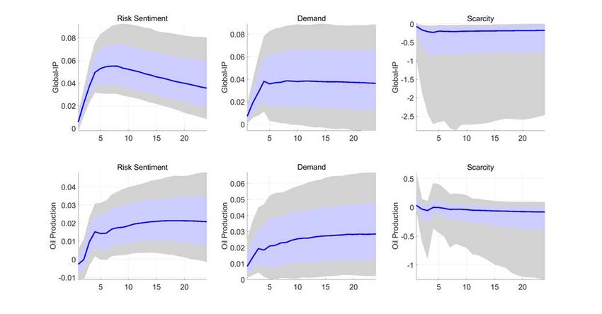
Figure 1: Oil Prices, global stock returns and slope of the futures curve
Notes: The scatter reports the daily percentage change of the oil price (Brent quality) on the horizontal
axis versus the daily percentage changes in global airline stock prices (vertical axis, left hand side
panel) and the difference between the percentage change of futures and spot oil prices (vertical axis,
right hand side panel).

market in days when this change is (i) large, (ii) negatively correlated with changes in the
price of oil (iii) positively correlated with the price of gold and with implied volatility in
the oil market.3 These are days when, in response to negative news on the global economy,
market participants run to safety, volatility in oil and stock markets spikes and the price
of oil plunges (alternatively, these are days in which positive news about global growth
raise oil prices and suppress volatility in financial markets).4 The external instrument
has, by construction, a sparse structure as it presents many zeros.5 The second shock is
an unexpected change in the current state of the business cycle and, as consequence, in
the demand for commodities. We identify this shock by conjecturing that it induces a
positive correlation between oil (both spot and futures) and stock prices but a negative
   3
     Volatility in equity markets is measured by the VIX, that is the CBOE Volatility Index. Implied
volatility in oil markets is captured by the OVX, which measures the market’s expectation of 30-day
volatility of crude oil prices by applying the same methodology used for the VIX to options on crude oil
futures. As shown by (Robe and Wallen, 2016) the VIX index is positively associated with the OVX, as
generalized financial uncertainty and oil market uncertainty indeed tend to move together.
   4
     Although the VIX is specific to the US S&P 500, it has a correlation as high as 0.9 with implied
volatility in European and Asian stock markets (Londono and Wilson, 2019). By using the VIX to gauge risk
sentiment in global markets we also follow a growing literature in applied macroeconomics (Kalemli-Ozcan,
2019).
   5
     The potential challenge from using sparse instruments is discussed in Budnik and Gerhard (2020), who
suggest resorting to Bayesian proxy VAR approaches.

ECB Working Paper Series No 2472 / September 2020                                                       7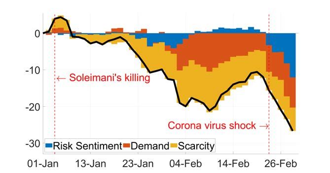
correlation between the price of oil and the slope of the futures curve. In other words,
conditional on this shock, spot and futures oil prices move in the same direction as stock
prices, but spot prices move more than futures prices. These two shocks (risk sentiment and
current demand) have broadly similar macroeconomic consequences, in that they both raise
economic activity and oil prices at the same time. In Schnabel (2020) parlance they are
both “demand” shocks. There are three good reasons for separating them. The first is that
risk sentiment shocks induce a much stronger positive correlation between oil, risky asset
prices and long-term bond yields. The second is that they have different implications for the
slope of the futures curve. The slope is broadly unaffected by risk sentiment shocks (that
raise current and futures prices by a similar amount) but is negatively related to current
demand shocks (that affect current prices more than futures prices). The third is that
risk sentiment shocks are found to have a much stronger impact on the price of inflation
swaps, from which popular measures of long-term inflation expectations are derived. These
shocks, therefore, help us in shedding some light on the somewhat puzzling link between
the price of oil and long-term inflation expectations, a point to which we return in Section
5. The last shock that we identify is a stagflationary disturbance, conditional on which oil
prices co-move negatively with stock prices. We term this structural disturbance a “scarcity”
shock. This shock conflates two structural shocks that have been studied extensively in
the oil price literature. The first is a supply shock, that is an unexpected exogenous fall
in the production of oil. This would raise the price of oil and induce a fall in economic
activity and also affect negatively stock returns (Kilian and Park, 2009). The second is
a shock to the precautionary demand for oil, due for instance to worries about future oil
availability. This is related more to uncertainty about the outlook for oil supply rather than
to current supply conditions, and has been typically associated with geopolitical tensions
involving large oil producing countries. Differently from the oil supply shock, uncertainty
about future oil supply leads to an increase in current oil production (Kilian and Murphy,
2014). This additional oil production, however, does not reach consumers and firms but
feeds higher inventories, leading again to a contraction in economic activity, and to a fall
in stock prices (Anzuini, Pagano, and Pisani, 2015). While we see some merits in trying
to distinguish these two sources of oil price fluctuations, we prefer treating them as a
single shock for two reasons. First, many episodes of geopolitical tensions involving large

ECB Working Paper Series No 2472 / September 2020                                            8
oil producers tend to include a combination of both actual oil supply disruptions as well
as worries about future oil availability. For instance, on the 14th of September 2019 oil
production facilities in Saudi Arabia were struck by drones and missiles and forced to shut
down. Besides causing a significant loss in actual production (about 5% of global output)
the attack also raised fears of further geopolitical tensions, increasing uncertainty on future
oil supply. In such a case, trying to separate the effects of actual supply shortfalls from
precautionary demand is challenging. Second, the macroeconomic implications of these two
shocks are not easily distinguishable. In fact, following both a negative oil supply as well as
a precautionary demand shock, oil is both scarcer and more expensive for both consumers
and producers, either because of lower production or because of higher storage needs. As a
result, economic activity and stock prices fall and the inflationary pressure due to higher
energy prices is somewhat offset by lower aggregate demand. These effects, and their real
time assessment, is what ultimately matters both for monetary policy makers, as well as
for market participants.
    The method described so far provides a daily decomposition of the price of oil in
structural shocks. However, nothing ensures that the shocks that we obtain from such a
daily VAR are consistent with the behaviour of prices and quantities in the physical oil
market. In particular, we would expect both demand shocks in our model to be associated
with an expansion in global economic activity and to induce an increase in oil production.
At the same time, the scarcity shock should cause a reduction in global economic activity.
Yet, it is not possible to have control over these effects when considering only the variables
in our daily VAR. By moving from traditional models of the physical oil market to a
framework in which oil is related to financial asset prices, we gain a real-time estimate of the
shocks, but lose touch with the fact that oil is a physical commodity. We re-establish such
consistency by introducing a second step in our identification procedure. For each candidate
structural model in the daily VAR, we extract the structural shocks and take their monthly
average. Conditional on demand shocks we require oil production and economic activity
to be positively correlated with the price of oil, while scarcity shocks need to induce a
negative correlation between oil prices and economic activity. Crucially, this second step is
only used to select, across all the candidate structural shocks derived in the first step, the
ones that have reasonable macroeconomic consequences and does not hinder the real time

ECB Working Paper Series No 2472 / September 2020                                              9
nature of the structural decomposition.
We use the model to analyze fluctuations in the oil price and their relationship with
global financial markets (equities, bonds, inflation swaps and currencies) using data between
June 2007 and February 2020. We find that risk sentiment shocks induce a parallel shift of
the oil futures curve: a one percent increase in the price of oil due to a risk sentiment shock
is associated with a rise of about one percent in 12 months ahead futures prices. More
generally, a positive risk sentiment shock raises global stock prices, reduces volatility, raises
interest rates as well as inflation expectations and leads to a depreciation of typical safe
haven currencies, namely the USD, the Japanese yen and the Swiss franc. The effects of
current demand shocks are qualitatively similar to, but quantitatively very different from,
those of risk sentiment shocks. They have very small effects on oil prices futures and, as
consequence, a strong negative impact on the slope of the futures curve, explaining most
of the negative correlation shown in the right hand panel of Figure 1. The response of
financial asset prices to a positive current demand shock is consistent with an improved
macroeconomic environment. Stock prices and bond yields rise, while volatility falls. Safe
haven currencies depreciate, but less than in response to risk sentiment shocks. Importantly
long-term market based inflation expectations do not respond to these shocks, suggesting
that the information content of risk sentiment and current demand shocks is indeed different.
Finally, an increase in the price of oil due to a negative scarcity shocks is associated with a
fall in risky asset prices, an increase in financial volatility and a depreciation of the dollar.
In general, however, the effect of scarcity shocks on financial asset prices is quantitatively
very limited. Long-term inflation expectations constitute an important exception, as they
respond significantly, albeit with a delay, also to scarcity shocks, suggesting that the latter
might shift inflation risk premia.
As a final exercise, we illustrate how the model could have been used in real time to
analyze the structural drivers of oil price developments between January and February 2020.
This period was characterized first by a marked increase in crude prices, as geopolitical
tensions between the US and Iran spiked following the killing of the Iranian general Soleimani
by a US drone, then by a collapse of oil (and financial) markets due to the Corona virus.
Our model neatly distinguishes the main drivers of the price of oil around these episodes,
attributing the rise in early January to scarcity shocks and the bulk of the Corona virus
ECB Working Paper Series No 2472 / September 2020 10related collapse to a combination of risk sentiment and current demand shocks.
The paper is structured as follows. Section 2 places our paper in the context of the
relevant literature. Section 3 describes the empirical model and the identification strategy.
Section 4 briefly discusses model estimation, deferring most of the details to a technical
Appendix. Section 5 presents the empirical results. Section 6 concludes.
2 Relationship with the literature
The first strand of the literature to which we relate includes a set of papers that use
Structural Vector Autoregressions to study global oil markets dynamics. Challenging the
conventional wisdom that viewed oil prices as largely exogenous to global macroeconomic
developments, Kilian (2009) is the first to notice that the macroeconomic consequences of
oil prices fluctuations cannot be assessed separately from the underlying shocks that cause
them. Subsequent contributions have built on this idea and explored different identification
strategies, see for instance Lippi and Nobili (2012), Kilian and Murphy (2014), Anzuini,
Pagano, and Pisani (2015) and Juvenal and Petrella (2015). In recent years, the debate
has shifted on the relationship between identifying restrictions and demand and supply
elasticities in oil markets. Using two different approaches, both Caldara, Cavallo, and
Iacoviello (2019) and Baumeister and Hamilton (2019) argue that the price elasticity of
supply is higher than previously estimated, and emphasize the role that oil supply shocks
have in explaining oil price changes in the past forty years.
We add to this literature by developing a high frequency model that provides a bridge
between the global oil market and financial markets.6 Unsurprisingly, we are not the first
ones to think about the identification of oil price shocks at the daily frequency. Since oil
prices convey signals on global growth, real time information on their structural drivers can
be used, for instance, for portfolio allocation. For this reason, financial market practitioners
and academics have recently studied the nexus between oil prices and financial markets,
typically relying on a simple rule of thumb that classifies daily changes of oil prices as
6
Kilian and Park (2009) investigate the role of oil supply and oil demand shocks in determining
fluctuations of the US stock market, but at the monthly frequency. They find that the effects of supply
shocks on stock returns are negligible. Oil demand shocks, on the other hand, provide a direct stimulus for
the U.S. economy that outweighs, at least in the short run, the negative effects of higher oil prices.
8
ECB Working Paper Series No 2472 / September 2020 11either demand or supply driven, depending on whether they are positively or negatively
correlated with stock returns (Rapaport, 2014; Perez-Segura and Vigfusson, 2016). A
similar identification philosophy, but in the context of a dynamic factor model, underlies
the New York Fed Oil Market Report by Groen, McNeil, and Middeldorp (2013). A
central contribution to this literature is the one by Ready (2017), where oil production
is connected to appetite for risk and equity prices in a theoretical model. In his model
the comovement between oil prices, stock market returns and implied volatility in equity
markets is determined by exogenous shifts in risk aversion, global demand for oil and
supply shocks. These shocks are then estimated in a SVAR with recursive ordering based
exclusively on asset prices (equity returns of oil producing firms, the VIX and oil prices).
While the philosophy of our identification scheme is similar to the one in Ready (2017), we
go beyond the recursive ordering, hardly tenable in a daily setting with financial market
variables. We construct a more credible identification scheme in which exogenous changes in
the risk attitude of investors are inferred from information contained in the joint movement
of volatilities in the stock and in the oil market, complemented with a narrative approach.
The fact that in our model all the variables can react contemporaneously to structural
shocks makes the resulting structural decomposition more credible. Importantly, none of
these high frequency papers tries to establish some consistency between the role that oil
plays in financial markets and the fact that oil is a physical commodity.
3 Shocks Identification
Our daily model is a three-variate Vector Autoregression that includes the price of oil,
airline stock prices and the price of the 12 months ahead oil futures. Our measure of the
price of oil is the log of Brent (1st futures delivery price). Global equity prices are the
log of the MSCI World Airline index7 . Futures prices are the log of the 12 months ahead
Brent futures. The sample runs from the 1st of June 2007 to the 28th of February 2020.
Collecting the n variables in the vector yt , we can write the structural representation of the
7
The MSCI World Index is a market cap weighted stock market index of the major world airlines.
ECB Working Paper Series No 2472 / September 2020 12model, which allows for contemporaneous interaction of the variables:
A 0 y t = A + xt + e t , et ∼ i.i.d. N (0, I), (1)
0 0 0
where A+ = [A1 , A2 , ..., Ap , c] and xt = [yt−1 , yt−2 , ..., yt−p , 1]0 . A0 is an n × n matrix of
contemporaneous interactions, the p matrices Aj (j = 1, 2, ..., p) of dimension n × n collect
the autoregressive coefficients, c is an intercept term and et is an n dimensional vector of
structural shocks. The reduced form model has a compact representation:
yt = Φ+ xt + ut , ut ∼ i.i.d. N (0, Σ),
where Φ+ = A0 −1 A+ and reduced form and structural shocks are related as follows:
ut = A−1
0 et = Bet , (2)
Σ = (A00 A0 )−1 . (3)
The matrix B, the structural impact matrix, is the crucial object of interest in structural
identification. To estimate this matrix we place three types of restrictions: restrictions on
the response of daily data to the shocks; restrictions on the response of monthly data to
the shocks; an upper bound on the elasticity of oil supply; narrative sign restrictions.
3.1 Identification restrictions on daily data
Risk sentiment shock. Motivated by Ready (2017), the first structural shock that we
analyze can be seen as a change in the willingness of market participants to bear risk due to
a substantial change in their assessment about future economic conditions. The importance
of investors’ sentiment in driving the high-frequency correlation between stock and oil prices
appears often in market commentaries and is also used by policymakers to rationalize, in
real time, the nature of the shocks that hit the economy. Bernanke (2016), for instance,
explicitly makes this point in his Brookings blog discussing the positive correlation between
stock returns and the price of oil: “[...] recent market moves have been accompanied by
elevated volatility. If investors retreat from commodities as well as stocks during periods
ECB Working Paper Series No 2472 / September 2020 13of high uncertainty and risk aversion, then shocks to volatility may be another reason for
the observed tendency of stocks and oil prices to move together.” The Brexit referendum
offers a concrete example of the type of shock we are after. On the first trading day after
the referendum (24th of June 2016) markets were shaken by increased uncertainty and
higher pessimism on future economic activity; implied volatility in the US stock market
jumped by 8.5 percentage points and world equities and the price of oil plunged by 5%. Our
first structural shock is designed to catch exactly episodes of this type, characterized by a
tight positive (negative) correlation between the price of oil and stock returns (financial
volatility).
While financial market participants agree that this is an important driver of the
correlation between the price of oil and asset prices, most economists would disagree on the
exact definition of such a shock. Arguably, one could think that such a co-movement in
asset prices could be prompted by first moment shocks like for instance the news shocks
identified by Kurmann and Otrok (2013), but also by second moment shocks, like for
instance the uncertainty shocks studied by Bloom (2014), Caldara, Cavallo, and Iacoviello
(2019), Alessandri and Mumtaz (2019) and Cesa-Bianchi, Pesaran, and Rebucci (2018). All
these different shocks are combined by Bluwstein and Yung (2019) in a “risk perceptions”
shock, that is an exogenous increase in the risk-premium that investors require to bear
risk. This shock depresses output and credit and raises implied volatility in stock markets.
Such a shock could originate from (i) a revision of expectations about future growth or (ii)
revisions of the balance of risks on growth or (iii) a combination of the two. We see this
shock as a disturbance that would induce investors to treat commodities in their portfolios
as if they were a risky asset (i.e. an asset whose returns are positively correlated with
future consumption).
To identify this shock we use an external instrument, in the spirit of Mertens and Ravn
(2013) and Stock and Watson (2012). The construction of the instrument proceeds in two
steps. First, we select, through a statistical procedure, days in which we observe a large
increase (decrease) of volatility in oil and equity markets and in the price of gold, and a
large decrease (increase) in the price of oil. Changes in the price of gold have been used to
isolate shocks to uncertainty (Piffer and Podstawski, 2018) and can be used as an indicator
of risk on/off mood in financial markets. Specifically, we consider, for each year in our
ECB Working Paper Series No 2472 / September 2020 14sample, the joint empirical distribution of daily gold and oil price returns and changes
in the VIX and in the OVX. We then select the days in which the change in all these
variables is large, based on a subjective statistical criterion. By ‘large’ we mean that they
fall, respectively, either below their 10th percentile or above their 90th percentile. In the
second step, we rely on market commentaries to assess the origin of such shock according to
financial market sources (Bloomberg, private sector newsletters and the IMF daily Global
Markets Monitor). This cross-check reveals that these specific days were characterized
by important revisions of global growth prospects. Operationally, we define our external
instrument as a variable equal to the actual change in the VIX in these days, and zero on
all other days in the sample.
After auditing the candidate dates through market commentaries, we are left with 15
days (see Table 1).8 In 2008-2019 we select five days, central in the unfolding of the global
financial crisis, with marked financial volatility and large moves in gold prices. In August
2011 a reduction of the US credit rating by Standard & Poor’s fueled concerns that the
ongoing economic slowdown could worsen. Ten days later the eruption of the euro area
crisis led to another spike in financial volatility that also negatively impacted oil prices.
Days of market turmoil in 2012 were dominated by disappointing news on growth prospects
for the US and for the euro area. Finally, in 2016 and in 2018 we identify as risk off
episodes the day of the Brexit referendum and a specific day in April 2018 when trade
tensions between the United States and China concretely intensified. In 2019 the trade war
escalation is picked up by several dates, following specific Trump tweets and the threat of
China retaliation. Finally, the 24th of February is picked up as the outbreak of the corona
virus shock.
Current oil demand. Our second shock of interest is an unexpected change in the
current state of the business cycle and, as a consequence, in the current demand for oil.
We identify this shock through sign and magnitude restrictions. First, we assume that an
increase in the demand for oil has a positive impact on the spot price of oil as well as on
equity prices. Second, we assume that a shock to current demand affects the price of oil at
all maturities, i.e. not only the spot price but also futures prices, but that its impact is
8
In Appendix A we report a full account, sourced from these market commentaries, of the key events
that, in each of these days, triggered a change in global risk appetite.
ECB Working Paper Series No 2472 / September 2020 15Table 1: Selected dates defining the external instrument
event date key headline OVX VIX Gold Oil
30-Sep-2008 Rescue package hopes -4.7 -7.3 -2.3 4.4
06-Oct-2008 Global growth fears 8.6 6.9 2.7 -7.6
17-Feb-2009 Global growth fears 10.1 5.7 2.8 -5.3
20-Apr-2009 Global growth fears 4.7 5.2 1.8 -6.8
01-Jun-2010 Global growth fears 5.6 3.5 2.0 -2.6
08-Aug-2011 US sovereign downgrade 13.8 16.0 2.5 -5.3
18-Aug-2011 Euro sovereign 14.8 11.1 2.2 -3.3
07-Sep-2011 Global growth rebound -2.5 -3.6 -4.3 2.6
01-Jun-2012 Global growth fears 6.8 2.6 2.9 -3.4
24-Jun-2016 Brexit 3.2 8.5 3.9 -5.0
02-Apr-2018 Trade tensions 2.5 3.7 1.2 -3.8
23-May-2019 Trade tensions 5.6 2.2 0.9 -4.7
31-May-2019 Trade tensions 7.3 1.4 0.9 -3.6
14-Aug-2019 Global growth fears 2.6 4.6 1.1 -3.0
24-Feb-2020 Corona virus shock 3.7 8.0 1.9 -3.8
Notes: From left to right: event date reports the specific
date from our combination statistical and narrative se-
lection criteria for the “risk dates”; key headline reports
the main risk driver identified from our reading of the
daily market commentaries; OVX, VIX, Gold and Oil,
report the daily change for the variable indicated (log
change for Gold and Oil). Source: authors’ compilation
from Bloomberg, Refinitiv, and other news reports.
relatively stronger for shorter than for longer maturities. This translates into an identifying
assumption on the slope of the futures curve, which we expect to go relatively more in
“backwardation” (i.e. sloping downwards) following a positive current demand shock and
more in “contango” (i.e. sloping upwards) following a negative demand shock. In other
words, conditional on a current demand shock, the spot price is negatively correlated with
the slope of the futures curve. Our assumption is that, everything else equal, a current
demand shock changes the market balance relatively more in the present than in the future,
so that the spot price has to adjust more than futures prices to clear the market.
Oil scarcity shock. The third structural shock is a supply driven exogenous tightening
of the oil market. This can occur for two reasons. The first is an exogenous disruption in
ECB Working Paper Series No 2472 / September 2020 16oil production, due for instance to geopolitical tensions, a natural disaster or a decision
of oil producers to cut production independently from demand conditions. These are
not rare events; Caldara, Cavallo, and Iacoviello (2019), for instance, identify 29 such
episodes between 1985 and 2011. There is a large consensus in the literature that such a
shock has stagflationary macroeconomic consequences, i.e. it yields higher oil prices and
higher inflation while leading to a contraction in economic activity. Yet scarcity of oil
for consumers and producers can also stem from higher demand for oil storage, i.e. from
a precautionary demand for oil driven by uncertainty about future oil supply (Anzuini,
Pagano, and Pisani, 2015). As explained in the Introduction, we conflate these two shocks
into a single stagflationary disturbance, a “scarcity” shock, which we identify by assuming
that it induces a negative conditional correlation between the price of oil and equity prices.
This assumption resonates with similar assumptions in the high frequency literature (Perez-
Segura and Vigfusson, 2016; Rapaport, 2014) and is supported by the theoretical model in
Ready (2017).
Narrative restrictions on the scarcity shock. We further sharpen the identification
of the scarcity shock with two additional narrative restrictions, in the spirit of Antolı̂n-
Dı̂az and Rubio-Ramı̂rez (2018). On the 14th of September 2019, a drone attack hit
the state-owned Saudi Aramco oil processing facilities in Saudi Arabia. The damage to
the production facility led to a substantial, albeit temporary, cut of Saudi Arabia’s oil
production, amounting to about 5% of global oil output. As a result, as markets opened
the following Monday (the 16th of September) the price of oil jumped by 13 percent, from
60 to 68 USD per barrel. We use this episode to place two identifying narrative restrictions
on the scarcity shock.
• Narrative Restriction #1: sign of the shock. On the 14th of September 2019 the
scarcity shock gave a positive contribution to the increase in the price of oil.
• Narrative Restriction #2: contribution of the shock. On the 14th of September 2019
the scarcity shock accounted for most of the change in the price of oil.9
9
In the following days worries about oil supply quickly retreated, as Saudi Arabia’s energy minister
pledged the use of strategic reserves to stabilise oil exports. Since we use daily data this does not represent
a problem for our identification strategy.
ECB Working Paper Series No 2472 / September 2020 173.2 Restrictions on monthly variables and elasticity bounds
So far, we have sought to identify primitive shocks to the price of oil by using information
exclusively from daily financial market data. Although we claim that the identification
restrictions that we have placed on daily data are plausible, one may wonder whether the
shocks that this identification scheme delivers have sensible implications for macroeconomic
variables as well as for the physical oil market. For instance, current demand shocks should
induce a positive correlation between oil prices, global economic activity and oil production.
We have also motivated our identification of scarcity shocks by arguing that they should
move oil prices and global economic activity in opposite directions. To ensure that our
shocks have these desired properties, we need to impose additional identifying assumptions
on the response of monthly variables (namely oil production and global economic activity)
on the structural shocks. A second, related point is that sign restrictions by themselves are
not sufficient to identify structural shocks in the physical oil market (Kilian and Murphy,
2012) and that imposing credible bounds on the elasticities of demand and supply narrows
down the set of plausible structural models.
We address both of these points. First, we add a set of identifying assumptions on the
response of oil production and global economic activity to demand and scarcity shocks. At
each point in time we compute an aggregate “macro demand” shock as the sum of the risk
sentiment and current demand shock. We then require both oil production as well as global
industrial production to co-move positively with the price of oil conditional on this shock.10
In response to a scarcity shock, on the other hand, we require global industrial production
to co-move negatively with oil prices. Second, we place an upper bound on the elasticity of
oil supply to limit the range of acceptable structural models. We place this upper bound
at 0.1. This value strikes a balance between the very low bound of 0.0258 set by Kilian
and Murphy (2014) and the evidence presented by Caldara, Cavallo, and Iacoviello (2019)
that this elasticity might be as high as 0.08. In our sample, results are not particularly
sensitive to the value chosen for this upper bound, as the posterior distribution of this
supply elasticity is concentrated towards the lower end of these values. A summary of the
10
We measure oil production as the world production of crude taken from the International Energy
Agency. As a proxy for global economic activity we use the industrial production based measure developed
by Baumeister and Hamilton (2019).
ECB Working Paper Series No 2472 / September 2020 18identification restrictions is presented in Table 2. We have populated the first column of
this table, which relates to the impact of the risk sentiment shock on the high and low
frequency variables, with the word ‘Proxy’, to clarify that the response of both the daily
and monthly variables to this shock is determined by the external instrument.
Table 2: Summary of the Identifying Restrictions
Risk sentiment Current demand Scarcity
Daily Model
Oil Price Proxy + +
Equity Prices Proxy + -
Oil price futures (12m) Proxy +
Monthly Model
Oil Production Proxy +
Global IP Proxy + -
Additional Restrictions
- Magnitude restriction: current demand shocks affect spot more than futures oil prices
- Narrative restrictions on the scarcity shock (14th of September)
- Upper bound (0.1) on the elasticity of oil supply
4 Model Estimation
The model is estimated using Bayesian methods. Here we briefly explain the main estimation
steps and refer the reader to Appendix B for all the technical details.
Shocks identification requires the estimation of the reduced form parameters Φ+ and Σ
and of the three columns of the structural impact matrix B = [b1 , b2 , b3 ]. The estimation of
these parameters is conceptually split in three steps. The first step consist of estimating the
reduced form parameters and the first column b1 using the external instrument described
in Section 3.1. We draw on the literature on Proxy-SVARs to estimate these parameters,
and in particular on the method developed by Caldara and Herbst (2019).
In the second step we use sign restrictions to set-identify b2 and b3 conditional on the
estimate for b1 obtained in the first step. Methods that tackle this problem have been
developed by Cesa Bianchi and Sokol (2017), Braun and Brggemann (2017) and Arias,
ECB Working Paper Series No 2472 / September 2020 19Rubio-Ramirez, and Waggoner (2019). In Appendix B we provide a detailed description of
how we adapt the procedure by Cesa Bianchi and Sokol (2017) to the Bayesian framework
of Caldara and Herbst (2019). In this step we also implement narrative sign restrictions on
the scarcity shock, rejecting all the candidate structural models in which scarcity shocks are
not the predominant contributors to the spike in the price of oil on the 14th of September
2019.
The final step consists of adding identification restrictions on lower frequency variables.
These are implemented by estimating the effects of the shocks (identified on daily data
and then averaged at the monthly frequency) on two monthly variables, namely global oil
production and global industrial production, and by discarding the candidate structural
shocks that do not satisfy either the sign restrictions on the monthly variables or the
elasticity bounds. Intuitively, this final step requires nothing more than a local projection of
the monthly variables on the identified shocks, and is performed along the lines of Jarocinski
and Karadi (2019), Paul (2017) and Gazzani and Vicondoa (2020). Crucially, this last step
does not hinder the real time nature of the structural decomposition, as the information
sets in the daily and in the monthly data do not need to be aligned. To give a concrete
example, in our empirical analysis the daily information set runs from the 1st of June
2007 to the 28th of February 2020, while data on global industrial production and on oil
production are only available up until November 2019. From the daily model we obtain a
range of candidate structural shocks up to the 28th of February 2020. For each of these
candidate shocks we run the (monthly) local projections with data up to November 2019.
Finally, out of the daily candidate shocks, we only keep those for which the (monthly)
local projections satisfy the sign restrictions and the elasticity bounds. In other words,
monthly information is only used to select, among the daily candidate shocks, those that
have reasonable macroeconomic implications.
5 Results of the empirical analysis
We organize the empirical section in four parts. We start by looking at Impulse Response
Functions for daily data. We then analyze the response of a wide array of financial variables
to our structural shocks. Then, we zoom in on some specific episodes of particular interest
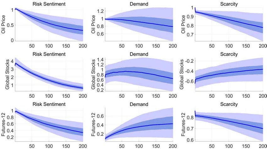
ECB Working Paper Series No 2472 / September 2020 20Figure 2: Impulse Response Functions for the daily VAR
Note. 68 percent confidence bands. Both parameter and identification uncertainty is reflected in the
confidence bands. Impulse response functions are standardized so as to lead to a 1 percent increase in
the price of oil.
for the interplay between oil and financial markets and interpret them through the lens
of our model. Finally, we describe how the model could have been used in real time do
understand oil price dynamics in a longer period, between January and February 2020,
when the killing of the Iranian general Soleimani by US forces first, and the spreading of
the corona virus afterwards, lead to pronounced volatility in oil markets.
5.1 Impulse Response Functions
Figure 2 shows the response of the endogenous variables included in the daily VAR to the
three structural shocks. Impulse response functions are normalized to generate a 1 percent
increase in the price of oil.
The risk sentiment shock. Since the IRFs are normalized so as to generate a rise in
oil prices, the first column of Figure 2 shows the effects of a positive risk sentiment shock. It
is worth remarking that these are estimated through an external instrument, so that neither
the sign nor the magnitude of these responses is, a priori, constrained. A striking result
is that a 1 percent increase in the spot price of oil is associated with a 1 percent increase
in the price of oil futures as well as in airlines stock prices. Two implications follow. The
first is that this shock captures indeed episodes of strong contemporaneous co-movement
between oil and stock prices. The second is that, in response to a risk sentiment shock,
ECB Working Paper Series No 2472 / September 2020 21the slope of the futures curve barely changes. This means that the shock that we are
capturing through our exogenous instrument is strongly forward looking and induces an
almost parallel shift of the futures curve.11
Current demand shock. The second source of positive correlation between oil and
stock prices is the current demand shock. There are three major differences in the way
this shock affects oil and stock prices as compared to the risk sentiment shock.12 First, the
increase in oil and stock prices is much slower and more persistent than what observed after
a risk sentiment shock. Second, oil prices rise relatively more than (about three times as
much as) stock prices. Third, this shock has a much stronger impact on spot than futures
oil prices. As the spot price of oil rises on impact by 1%, oil price futures only rise by
around 0.1 percent, and thus the slope of the futures curve declines significantly. As a
result, this is the shock that is mostly responsible for the negative correlation between spot
and futures prices shown in the right hand side panel of Figure 1.
Scarcity shock. Conditional on a scarcity shock, a 1 percent increase in the price of
oil is associated with a significant fall in stock prices (-0.45 percent). Futures prices also
respond strongly to this shock, although their reaction is milder than that of spot prices
(0.8 percent). This implies that part of the negative relationship between spot prices and
the slope of the futures curve in Figure 1 is also due to supply side shocks.
In Appendix C we describe in details the effects of the structural shocks on monthly
variables, in particular oil production and the measure of global industrial production
developed by Baumeister and Hamilton (2019). This analysis shows that risk sentiment
and current demand shocks have broadly similar macroeconomic consequences, as they
raise persistently both industrial production and oil production. The latter responds to risk
sentiment shocks only with a lag, suggesting that this disturbance anticipates macroeconomic
developments that lead to higher demand for oil, which in turn is accommodated by higher
oil production. Scarcity shocks, on the other hand, have a significant recessionary impact
but do not have a significant effect on oil production, as they blend shocks (supply and
11
Understanding whether this is due to risk premia or to changes in the convenience yields rather than
to expectations would require a term structure model. While this question is of great interest it a beyond
the scope of our analysis.
12
We should note that, despite the same pattern of signs for the risk sentiment and demand shocks
estimated from our IRFs, we are still able to separately identify the the demand shock from the risk shock:
demand shocks are, by assumption, orthogonal to the proxy used for the identification of risk sentiment
shock (Arias, Rubio-Ramirez, and Waggoner, 2019).
ECB Working Paper Series No 2472 / September 2020 22precautionary demand) that move production in opposite directions.13
5.2 Impact on financial variables
This section, the heart of our empirical analysis, illustrates how our identified structural
shocks shape the relationship between the price of oil and global financial markets. To this
end, we run a battery of local projections of various asset prices on the identified structural
shocks. The exercise follows in spirit Kilian (2008) and Kilian, Rebucci, and Spatafora
(2009), who study the effects of oil price shocks on output, inflation and external balances.
To measure the dynamic effect of the shock St on a particular asset price yt , h days
after the shock, we estimate regressions of this form:
yt+h = αh + βh Zt−1 + γh St + uht , h = 0, 1, . . . , H, (4)
where Zt is a set of controls and uht is a residual. The parameter γh is an estimate of the
impulse response function of the variable yt to the shock St at horizon h (Jorda, 2005). In
all of our specifications the controls Zt include p lags of the endogenous variable14 together
with the variables included in the daily VAR, namely spot and futures oil price and global
airline stock prices. Since shocks are identified up to a sign, we standardize the coefficient
γh by the contemporaneous effect of the shock St on the percentage change in the price of
oil. This makes these regression coefficients directly comparable to the impulse response
functions shown in figure 2, which are similarly standardized. For each asset price, and
for each shock, we estimate local projections up to 90 days following the shock, namely
h = 1, . . . 90.15 We analyze five markets: equity, sovereign bonds, inflation swaps, foreign
exchange, and other commodities.
Equity markets. We start by analyzing the response to the identified structural
shocks of several (log) equity market indices (US, China, Euro area, UK, Japan, a global
13
Forecast error variance decomposition are not reported for the sake of brevity, but are available upon
request.
14
The projection regressions are estimated using Bayesian methods. We report results for p = 1. Adding
further lags does not change the outcome of the analysis.
15
Notice that St is a generated regressor. We therefore estimate its effects using the following algorithm.
First, we obtain a draw of St from the posterior distribution of the daily VAR. Then, conditional on this
draw, we draw 100 estimates of γh using a standard regression model with conjugate, uninformative, priors.
We repeat this procedure 250 times and thus obtain an empirical distribution for γh .
ECB Working Paper Series No 2472 / September 2020 23aggregate), of implied volatility in the US (the VIX) and of implied volatility in Europe (the VSTOXXI, see Figure 3). The first, important, result is the strong response of equity prices to a risk sentiment shock. Strikingly, equity prices for China (and also, not shown in the chart for brevity, for EMEs) rise by 1 percent on impact, given a 1 percent increase in the price of oil, revealing a tight link between investors sentiment on Emerging markets and oil prices. Current oil demand shocks also have a strong, positive effects on equity prices, but their impact response is around one third that of risk sentiment shocks, confirming that it is the latter shock that captures the bulk of the positive co-movement between equity and oil prices. Equity prices tend to respond negatively to scarcity shocks across the board, but the effect is smaller and less precisely estimated (significant only for Europe, Japan and China). ECB Working Paper Series No 2472 / September 2020 24
You can also read