Sovereign Defaults: The Price of Haircuts
←
→
Page content transcription
If your browser does not render page correctly, please read the page content below
Sovereign Defaults:
                              The Price of Haircuts
                                       Juan J. Cruces*
                                 Universidad Torcuato Di Tella

                                    Christoph Trebesch§
                               University of Munich and CESIfo

                                               Abstract

           A main puzzle in the sovereign debt literature is that defaults have only
           minor effects on subsequent borrowing costs and access to credit. This
           paper comes to a different conclusion. We construct the first complete
           database of investor losses (“haircuts”) in all restructurings with foreign
           banks and bondholders from 1970 until 2010, covering 180 cases in 68
           countries. We then show that restructurings involving higher haircuts are
           associated with significantly higher subsequent bond yield spreads and
           longer periods of capital market exclusion. The results cast doubt on the
           widespread belief that credit markets “forgive and forget.”

           JEL Classification Numbers: F34, G15

           Keywords: Sovereign Debt Crises, Restructuring, Reputation

*
    Business School, Universidad Torcuato Di Tella, juan.cruces@utdt.edu.
§
    Dept. of Economics, University of Munich. christoph.trebesch@lmu.de. Corresponding author.
We thank Alexander Agronovsky, Paula Covelli, Isaac Fainstein, Andreea Firca, Federico Malek, Pablo
González Ginestet, Víctor Poma, Said Khalid Scharaf, Lina Tolvaisaite and Alexander Vatagin for
excellent research assistance at different stages of this project. We are also indebted to Peter Benczur,
Helge Berger, Kit Baum, Charlie Blitzer, Mustafa Caglayan, Henrik Enderlein, Barry Eichengreen,
Gaston Gelos, Eduardo Levy Yeyati, Andy Neumeyer, Andrew Powell, Guido Sandleris, Julian
Schumacher, Beatrice Weder di Mauro, as well as participants at the Berlin Conference on Sovereign
Debt and Default, the Royal Economic Society Meetings 2011, the XIII Workshop in International
Economics and Finance, the DIW Conference on the Future Role of Finance and the XVI World
Congress of the International Economic Association for helpful comments. We thank Peter Benczur,
Cosmin Ilut, Federico Sturzenegger and Jeromin Zettelmeyer as well as Barclays Capital, Lehman
Brothers and Moody’s for kindly sharing data. Trebesch gratefully acknowledges financial support from
the Fox International Fellowship Program (Yale University) and from the German Research Foundation
(DFG) under the Collaborative Research Centre 700. Part of this research was carried out while
Trebesch was visiting the IMF.
Parts of the data can be downloaded here: https://sites.google.com/site/christophtrebesch/data
1. Introduction
Theory predicts that sovereign defaults result in reputational damage and the
government’s exclusion from capital markets. 1 But empirical support for this
proposition is weak at best, as shown by 30 years of research. According to the
consensus of empirical studies, defaulting countries do not face substantially higher
borrowing costs after a debt crisis, and often regain access to borrowing in just two
years.2 These findings have led many to conclude that “debts which are forgiven will
be forgotten” (Bulow and Rogoff 1989b, p. 49). In this paper, we build and exploit a
comprehensive dataset on creditor losses (“haircuts”) in past debt restructurings and
come to a different conclusion. In contrast to earlier work, we find that sovereign
default is a main predictor of subsequent borrowing conditions, once the scope of
creditor losses is taken into account.
The paper is organized around its two contributions. The first part presents a new
database of haircut estimates, covering all sovereign debt restructurings with foreign
banks and bondholders between 1970 and 2010, the only complete set of estimates so
far. To construct this dataset we gathered and synchronized data from nearly 200
different sources, including the IMF archives, private sector research, offering
memoranda and articles from the financial press. The result is the first full archive on
sovereign restructuring events since the 1970s, providing not just haircut estimates,
but also details on the occurrence and terms of past restructurings, as well as the
characteristics of old and new instruments involved in each exchange. Like in
Sturzenegger and Zettelmeyer (2008) we use the collected restructuring details to
compute haircuts as the percentage difference between the present values of old and
new instruments, discounted at market rates prevailing immediately after the
exchange. To compute deal-specific “exit yields” for each restructuring since the
1
See Eaton and Gersovitz (1981) or, more recently, Kletzer and Wright (2000), Kovrijnykh and
Szentes (2007), Arellano (2008), D’Erasmo (2010), and Yue (2010). A different branch of the
literature suggests that sovereign defaults can have adverse spillover effects beyond sovereign credit
markets, e.g. on trade (Rose 2005), investment (Fuentes and Saravia 2010) or for the private sector in
the debtor country (Arteta and Hale 2008, Sandleris 2008). See also Cole et al. (1995) and Cole and
Kehoe (1998). Others study the possibility of direct sanctions (e.g. Bulow and Rogoff 1989a,
Mitchener and Weidenmier 2005, Tomz 2007).
2
See the surveys by Eaton and Fernandez (1995) and Panizza et al. (2009), as well as Eichengreen
(1989), Jorgensen and Sachs (1989), Lindert and Morton (1989), Özler (1993), Dell’Arriccia et al.
(2006), Borensztein and Panizza (2009) and Gelos et al. (2011).
11970s we also develop a new discounting approach, which takes into account both
the global price of credit risk and country conditions at each point in time.
We find that the average sovereign haircut is 37%, which is significantly lower than
for corporate debt restructurings in the United States (see section 3). We also find
that there is a large variation in haircut size (one half of the haircuts are below 23%
or above 53%) and that average haircuts have increased over the last decades. These
data and stylized facts are relevant from a policy perspective, as they enable more
informed judgments on debt crises outcomes and private creditor burden sharing in
the past decades. In addition, the dataset sheds new light on sovereign debt as an
asset class. In particular, it provides, for the first time, representative estimates on
sovereign debt recovery rates.3 These may be used for future academic research, but
also as inputs for a wide range of credit risk models in the financial industry, e.g. to
back out default probabilities from observable bond prices.
The second part of the paper documents the relationship between restructuring
outcomes and subsequent borrowing conditions for debtor governments. Our key
hypothesis is that higher haircuts are associated with (i) higher post-restructuring
spreads and (ii) longer duration of exclusion from capital markets. These predictions
can be derived from recent sovereign debt models which build on the seminal work
by Eaton and Gersovitz (1981).4 The intuition in these papers is straightforward. A
defaulting country that aims to resolve its debt crisis negotiates with creditors not
only on the size of the haircut, but also on the level of subsequent risk premia and on
the possibility to access credit in the future. The debtor faces a trade-off: A high
haircut implies a large degree of debt reduction now, but is punished by markets
tomorrow. To our knowledge this paper is the first to bring these theoretical priors to
the data.
3
Given the lack of data, even rating agencies continue to base their recovery assumptions for
sovereigns on a very small sample of restructurings. The most recent report by Moody’s (2011) shows
recovery rates on 15 recent cases, while Standard and Poor’s (2011) relies on estimates for 5
countries.
4
In particular Yue (2010), D’Erasmo (2010) and Asonuma (2011).
2Our econometric models analyze sovereign borrowing costs after debt restructuring
events. We start by running a fixed effects panel regression with monthly sovereign
bond spreads as the dependent variable, using the Emerging Market Bond Index
Global (EMBIG) for 47 countries, and then lag our haircut measure for up to seven
years after the restructuring. In a second step, we analyze the duration of exclusion
from capital markets by applying semi-parametric survival models. Our exclusion
measure captures the number of years from the restructuring until the country
reaccesses international capital markets. To improve on previous work on exclusion
duration we construct a yearly dataset of reaccess, which combines data on more
than 20.000 loans and bonds at the micro level with aggregate credit flow data at the
country level.
The results can be summarized as follows: In the benchmark specification with
country and year fixed effects a one standard deviation increase in haircut (22
percentage points) is associated with post-restructuring bond spreads that are 150
basis points higher in year one after the restructuring and still 70 basis points higher
in years four and five. These are sizable coefficients, especially when compared to
the findings of previous empirical work. In addition, we find that haircut size is
highly correlated with the duration of capital market exclusion. Ceteris paribus, a one
standard deviation increase in haircuts is associated with a 50% lower likelihood of
re-accessing international capital markets in any year after the restructuring.
We attribute our results to more precise measurement of a country’s repayment
record. Previous papers attempting to gauge the effects of defaults on subsequent
market access have used a binary default indicator, capturing any missed payment as
explanatory variable for past credit history.5 But recent models predict punishments
that are proportional to the loss inflicted on investors.6 Using binary default instead
of actual losses ignores the large variation in restructuring outcomes. This may be
one reason why past research concluded that punishment effects in sovereign credit
5
This applies to all papers cited footnote 2. Relatedly, a recent paper Benczur and Ilut (2009) uses
arrears as a continuous measure for repayment history.
6
See in particular, Yue (2010) who studies debt renegotiation dynamics with endogenous recovery
rates. Also Benjamin and Wright (2009) take into account the magnitude of default, and develop a
model that generates a positive correlation between delays in debt renegotiation and the size of the
haircut.
3markets are negligible, at least in the medium run. Our analysis indicates that it is
crucial to consider the magnitude of past defaults, not only the default event per se.
The rest of the paper is structured as follows. The methodology to compute haircuts
and a number of stylized facts from the resulting dataset are summarized in sections
2 and 3. Section 4 discusses theoretical considerations and the two testable
predictions. Section 5 assesses the link between haircuts and subsequent bond yield
spreads, while section 6 focuses on capital market exclusion. The last section
concludes.
2. Estimating Creditor Losses: Methodology and Data
This section summarizes the construction of our haircut database, which is presented
in detail in the Appendix. We provide two main sets of haircut estimates: one
following the approach used by most market participants (“market haircut”) and
another using the more refined approach of Sturzenegger and Zettelmeyer (“SZ
haircut”) who estimate haircuts rigorously for 22 recent restructurings (see
Sturzenegger and Zettelmeyer 2006 and 2008, SZ hereafter). Other authors have
preceded us in providing haircut estimates – albeit with a more limited scope.7 Our
contribution is that we are the first to estimate haircuts based on a present value
approach for all 180 sovereign debt restructurings with foreign banks and
bondholders between 1970 and 2010. In addition, we collect data on nominal debt
reduction, measured as the share of debt written off to face value.
Section 2.1 defines the two main haircut measures, while section 2.2 summarizes
how we compute debt service streams and briefly presents our discounting approach.
Section 2.3 discusses case selection and the data sources used.
7
Jorgensen and Sachs (1989) were the first to compute creditor losses in sovereign restructurings
covering four cases during the 1930s and 1940s. Benjamin and Wright (2009) provide haircut
estimates for a large sample of 90 cases since 1990, which are not computed in present value terms
but rather based on aggregate face value reduction and interest forgiven. Further haircut estimates for
several recent cases are provided by Cline (1995), Rieffel (2003), Bedford et al. (2005), Finger and
Mecagni (2007) and Díaz-Cassou et al. (2008). In addition, some authors computed the internal rates
of return on sovereign bonds historically or over longer periods of time, but without computing
recovery values for specific restructurings: e.g. Eichengreen and Portes (1986, 1989), Lindert and
Morton (1989), Klingen et al. (2004) and Esteves (2007).
42.1. Defining Investor Losses
Debt restructuring typically involves swapping old debt in default for a new debt
contract. For a country i that exits default at time t and issues new debt in exchange
for old debt, and which faces an interest rate of at the exit from default, the market
approach to calculate haircuts (HM) is
1 (1)
This approach thus compares the present value (PV) of the new debt instruments
(plus possible cash repayments) with the full face value amount of the old
outstanding debt. This simple formula is widely used by financial market participants
and does not require detailed knowledge of the old debt’s characteristics. One reason
for using it as a benchmark is that debt payments are typically accelerated at a default
event.8 A more refined haircut measure has recently been proposed by SZ (2008):
1 (2)
The key difference between equations (1) and (2) is that unmatured old debt
instruments are not taken at face value but computed in present value terms and
discounted at the same rate as the new debt instruments. The rationale for using a
common discount rate for new and old instruments is that it reflects the increased
debt servicing capacity resulting from the exchange itself. Of course, when the old
debt had all fallen due at the time of the restructuring, HSZ uses the face value of that
old debt, just like HM, which happens in 92 of the 180 cases in the sample.
Furthermore, both formulae include past due interest on the old debt at face value,
but disregard penalties.
HSZ will be our preferred haircut measure for several reasons. In line with SZ, we
argue that equation (2) provides haircuts that better describe the “toughness” of a
8
Acceleration clauses entitle creditors to immediate and full repayment in case the debtor defaults on
interest or principal payments (see Buchheit and Gulati 2002).
5successful exchange than equation (1). Intuitively, HSZ compares the value of the new
and the old instruments in a hypothetical scenario in which the sovereign kept
servicing old bonds that are not tendered in the exchange on a pari passu basis with
the new bonds (SZ 2008, p. 783). More generally, SZ interpret their measure as
capturing the degree of pressure that must have been exerted on creditors to accept a
given exchange offer, so as to overcome the associated free rider problem. They also
argue that acceleration clauses might not always be a valid justification for taking the
old debt at face value, as done in equation 2. In fact, 77 of the 180 debt exchanges
were pre-emptive, that is, implemented prior to a formal default that could have
triggered acceleration. Another advantage of the HSZ approach is that it explicitly
accounts for portions of debt that have been previously restructured. It therefore
provides a better measure, compared to HM, of the cumulative losses afforded by
investors in a sequence of exchanges of the same debt.9 This is empirically relevant,
as many debtor countries restructured the same debt two or three times during the
1980s and early 1990s (see also Reinhart and Rogoff 2009 for a discussion of “serial
defaults”).
Equation (2) will often but not always yield a lower haircut estimate than equation
(1). The difference between these two measures arises from the comparison between
the face value and the present value of the old debt.10
2.2. Discounting Payment Streams
This section briefly summarizes our methodology to compute present values of both
the new and the old debt.
9
For example, if a country restructures old debt at time t but the new debt is renegotiated again soon
after, say at time t+N, then HM will depend on the product which will tend to
overestimate the cumulative loss of investors since in general < 1, especially when the debt
is long term. Under HSZ, this latter ratio would be which under normal conditions is much
closer to 1.
10
When is larger than the interest/coupon rate on the old debt, then HM > HSZ (76 cases in the
sample). This discrepancy will tend to increase, the longer the remaining maturity of the old debt.
When is smaller than the interest/coupon rate on the old debt, then the present value of the old debt
is greater than par and HM < HSZ (11 cases in the sample).
6Computing Contractual Payment Flows: We start by computing the contractual
cash flows in US dollars of the old and the new debt for each year from restructuring
to maturity. To do this, we collect detailed data on debt amounts, maturity,
repayment schedule, contractual interest/coupon rate and any further debt
characteristics that might influence an instrument’s value (such as the
collateralization of interest payments in Brady bonds).
In computing cash flows, we take advantage of the most disaggregated
information available. This means that we calculate present values on a loan-by-
loan and bond-by-bond level, whenever we could collect such information. For all
cases in which detailed terms were unavailable, as often happens in restructurings
of the 1970s and 1980s, we simply compute an aggregated discounted cash flow
stream and haircut for all of the debt. The Appendix provides further details,
including the scope of data available for each restructuring.
Discounting: We next discount the cash flow streams to assess their present values.
Most importantly, this requires choosing a discount rate for each restructuring. In
their analysis of major deals from 1998 until 2005, SZ use the secondary market
yield implicit in the price of the new debt instruments on the first trading day after
the debt exchange. Unfortunately, such market-based “exit yields” are only available
for a very small subsample of recent cases with liquid secondary debt markets. This
lack of data has pushed other researchers to use a constant rate across
restructurings 11 , despite the fact that countries restructured their debts in very
different conditions. 12
11
A popular rule of thumb is to use a flat 10% rate, as done, for example, by the Global Development
Finance team of the World Bank (Dikhanov 2004), by IMF staff (see Finger and Mecagni 2007) and
by researchers such as Andritzky (2006). Others have used risk free reference rates such as U.S.
Treasury bond yields or Libor (e.g. Claessens et al. 1992).
12
For example, when Nigeria restructured in 1991, its credit rating was 19.5 points on the Institutional
Investor scale (a scale that goes from 0 to 100 where larger numbers imply more creditworthiness),
while when South Africa restructured in 1993 its credit rating was 38.2. Hence, it is unlikely that the
default-exit yield would be the same for these two debtors. It is also well known that the credit risk
premium changes over time. For example, when Russia restructured in August 2000, the secondary
market yield on Moody’s index of speculative grade US corporate bonds was 11.43%, while it was
only 8.14% when Argentina restructured in 2005. Our procedure takes into account both of these
factors and gives different yields for these four cases: 9.81 for South Africa, 10.36 for Argentina,
12.48 for Russia and 18.28 for Nigeria.
7We also provide an original contribution to the literature in this front: we design a
procedure to impute voluntary market rates specific to each of the 180 restructurings
in our sample, thus covering more than three decades. Our imputed discount rates
take into account two main determinants of the cost of capital facing debt issuers at
the exit from default: a) the specific country situation and b) the level of the credit
risk premium at that time. In a nutshell, the procedure can be summarized as follows.
We start from secondary market yields on low-grade US corporate bonds which we
group by credit rating category. We then convert these corporate yields into discount
rates on sovereign debt by first linking corporate and sovereign secondary market
yields and then imputing yield levels for each sovereign based on its credit rating at
the time of restructuring. In the spirit of SZ, we then use these imputed discount rates
at the exit from default to discount the cash flows of the old and new debt. Overall,
the procedure yields monthly discount rates for all countries in our sample for the
period 1978 to 2010. To our knowledge, no set of estimates in the literature spans
such a large number of countries and years (see the Appendix sections A4.2 and
A4.3 for a detailed methodological description).
2.3. Data Sources and Sample
When starting this project there was no single standardized source providing the
degree of detail and reliability necessary to set up a satisfactory database of
restructuring terms since the 1970s from which to estimate haircuts. We therefore
embarked into an extensive data collection exercise, for which we gathered and
cross-checked data from all 29 publicly available lists on restructuring terms and
more than 160 further sources, including the IMF archives, books, policy reports,
offering memoranda, private sector research and articles in the financial press. The
Appendix provides an overview of sources used, describes our approach to minimize
coding errors and reports a data quality index for each deal. The detailed list of
sources on each restructuring is available upon request.
The case sample in this paper covers the entire universe of distressed sovereign debt
restructurings with foreign commercial creditors (banks and bondholders) from 1970
until 2010. To identify relevant events we apply five case selection criteria. First, we
8focus on sovereign restructurings, defined as restructurings of public or publicly
guaranteed debt. We do not take into account private-to-private debt exchanges, even
if large-scale workouts of private sector debt were coordinated by the sovereign (e.g.
Korea 1997, Indonesia 1998). Second, we follow the definition and data of Standard
and Poor’s (2006, 2011) and include only distressed debt exchanges. Distressed
restructurings occur in crisis times and typically imply new instruments with less
favorable terms than the original bonds or loans. We therefore disregard market
operations that are part of routine liability management, such as voluntary debt
swaps. Third, we focus on sovereign debt restructurings with foreign private
creditors, thus excluding debt restructurings that predominantly affected domestic
creditors and those affecting official creditors, including those negotiated under the
chairmanship of the Paris Club. Foreign creditors include foreign commercial banks
(“London Club” creditors) as well as foreign bondholders. For recent deals, we
follow the categorization into domestic and external debt exchanges of Sturzenegger
and Zettelmeyer (2006, p. 263).13 Fourth, we restrict the sample to restructurings of
medium and long-term debt, thus disregarding deals involving short-term debt only,
such as the maintenance of short-term credit lines, 90-day debt rollovers, or cases
with short-term maturity extension of less than a year. Finally, we only include
restructurings that were actually finalized. We thus drop cases in which an exchange
offer or agreement was never implemented, e.g. due to the failure of an IMF program
or for political reasons.
Based on these selection criteria, we identify 182 sovereign debt restructurings in 68
countries since 1978 (no restructurings occurred between 1970 and 1977). We were
able to gather sufficient data to compute haircuts on all of these cases, except for the
restructurings of Togo 1980 and 1983. We thus base all summary statistics on a final
sample of 180 implemented restructurings by 68 countries.
13
As a result, we do include two restructurings involving domestic currency debt instruments, but
only because they mainly affected external creditors: Russia’s July 1998 GKO exchange and
Ukraine’s August 1998 exchange of OVDP bonds.
93. Haircut Estimates: Results and Stylized Facts
The dataset and estimates of the 180 deals in our final sample reveals a series of new
insights on sovereign debt restructurings.
A first insight is the large variability in haircut size across space and time. Figure 1
plots our estimates of HSZ (eq. 2) over time and the respective, inflation-adjusted debt
volumes of each restructuring, as represented by the size of the circles.14 The graph
illustrates the dispersion in haircuts, which has increased notably since the 1970s.
Recent years have seen a particularly large variation, with some deals involving
haircuts as high as 90% and others involving haircuts as low as 5%. Interestingly, we
find that the three largest restructurings of recent years (Argentina 2005, Russia 2000
and Iraq 2006) all implied haircuts of more than 50%. But also the Brady deals of the
mid 1990s show high haircuts and involved large volumes of debt. A related trend is
illustrated in Figure 2, which differentiates between restructurings with some degree
of face value debt reduction (57 cases) and deals that only involved a lengthening of
maturities (123 cases). The figure shows that cuts in face value have become
increasingly common and that they tend to imply much higher creditor losses in
present value terms. Deals with outright debt write offs have an average haircut of
65%, compared to just 24% for pure debt reschedulings.
Table 1 provides further key insights, in the form of summary statistics for the full
sample of 180 restructurings. Most notably, we find the average SZ haircut between
1970 and 2010 to be 37% (simple mean), while the volume-weighted average haircut
14
Figure 1 shows that we estimate negative haircuts for a small subset of cases, most of which
happened in the first half of the 1980s. Negative haircuts typically result from a restructuring in which
the interest rate on the new debt exceeds the estimated discount rate prevailing at the time. In such
cases, any lengthening of maturities will increase the present value of the restructured debt, instead of
decreasing it (note that most deals in the 1980s involved rescheduling only). While these look like bad
deals for the government, a successful agreement can buy time and avoid a disorderly default. In
severe distress, these benefits can outweigh the drawback of accepting a deal at unfavorable terms.
10is even lower, amounting to about 30%. This implies that, on average, investors
could preserve almost two-thirds of their asset value in restructurings of the past
decades. This degree of losses is surprisingly low, at least when compared to
corporate debt exchanges. According to the most comprehensive set of estimates for
US corporate bond and loan restructurings (Moody’s 2006), the average haircut
between 1982 and 2005 was 64%. This is nearly twice as high as what we find for
sovereign debt. This large discrepancy is surprising, because US corporate debt, in
contrast to sovereign debt, can be enforced in courts and because any corporate
restructuring is subject to an orderly bankruptcy regime,
The table also shows notable differences in haircut estimates depending on the
formula applied. As expected, the market haircut tends to be larger than the SZ
haircut (40% vs. 37%, respectively). The difference between the two measures
ranges from 0 (for those 92 deals in which the old debt had fully matured) up to 22
percentage points. More specifically, the average HSZ is 6.5 percentage points lower
than the average HM for those cases in which the old debt had not fully come due.
Interestingly, creditor losses appear remarkably lower when looking at face value
reduction only, with an average haircut of only 16%. This low figure suggests that
any estimates based on nominal debt write-offs will severely overestimate the actual
recovery rates in sovereign restructurings. Also preemptive restructurings, i.e. those
implemented prior to a payment default, have significantly lower mean haircuts.
Looking at different decades, we find a notable increase in haircut size over time.
Average haircuts were about 25 percentage points higher during the 1990s and 2000s
as compared to deals implemented during the 1970s and 1980s. One reason is that
deals during the 1980s mostly implied maturity extensions only, thus postponing the
day of reckoning that most debtor countries had deep-rooted solvency problems.
Relatedly, we find that the Brady deals, which ultimately put an end to the 1980s
debt crisis for 17 debtor countries, involved a high average haircut of 45%. This
exceeds the mean investor loss for the more recent subsample of 17 sovereign bond
restructurings since 1998 (38%).
11The type of debtor also matters. In particular, we find average haircuts of 87% in
restructurings of highly indebted poor countries (HIPCs). To show this, we
categorize a subsample of restructurings as donor supported, defined as those co-
financed by the World Bank’s Debt Reduction Facility (see World Bank 2007).15 The
average haircut in these 23 donor supported restructurings is nearly three times as
large as for restructurings in middle income countries.
Table 2 shows our haircut estimates for 17 recent restructurings and compares them
to results of previous work. For the overlapping sample, our estimates are very
similar to those of SZ. When comparing their average haircut (reported in SZ 2006,
p. 263) to our equivalent of equation (2) we get a mean absolute deviation of 5.8
percentage points.16 We also find our results to be roughly in line with the net present
value estimates by Bank of Spain and Bank of England staff (Bedford et al. 2005 and
Diaz-Cassou et al. 2008), with a mean absolute deviation of 7.9 and 8 percentage
points, respectively. Our results differ more markedly from Finger and Mecagni
(2007), who apply a constant 10% discount rate, and from those reported by
Benjamin and Wright (2009), who do not calculate haircuts in present value terms
but base their estimates on World Bank data on debt stock reduction and interest and
principal forgiven.
4. Theoretical Considerations
Theoretically, we can refer to recent sovereign debt models that build on Eaton and
Gersovitz, in particular Yue (2010), D’Erasmo (2011) and Asonuma (2011) who
predict how haircut size affects subsequent access to foreign credit. Yue’s (2010) and
D’Erasmo’s (2009) model generate endogenous exclusion from financial markets
after default, where the duration of exclusion increases with the amount of debt
reduced. A bad credit record and a low recovery rate of the defaulted debt imply
15
The Debt Reduction Facility grants funds to governments to buy back their debts to external
commercial creditors at a deep discount. Typically, the size of haircuts granted by commercial
creditors is in the range of those accepted by official creditors in these same countries (World Bank
2007).
16
Only two estimates differ significantly (by more than 10 percentage points), namely Pakistan 1999
and Ukraine 2000, and this is mostly because our methodology yields significantly lower discount
rates for these two cases.
12longer exclusion. The models can be extended so that creditors and debtors bargain
not only over the size of the recovery rate, but also on the risk premium paid on debt
issues after re-entry into capital markets (see e.g. Asonuma 2011). Analogously, the
yield spread on new debt will be higher, the lower the implied recovery rate of the
restructuring, i.e. the higher the haircut. We can therefore derive two testable
hypotheses: Hypothesis 1: The larger the size of H, the higher the yield spreads after
restructurings; and Hypothesis 2: The larger H, the longer the period of exclusion
from capital markets.
The underlying mechanism suggested in these papers is the classic reputational one
in Eaton and Gersovitz (1981): A good repayment record assures access to credit in
the future, while defaulting will be punished. 17 However, there could be other
channels linking the size of haircuts and subsequent borrowing conditions.
First, there is the countervailing effect of debt relief. Sovereigns imposing high
haircuts will reduce their indebtedness more significantly, making them more
solvent, at least in the short run. In an atomistic bond market without creditor
collusion, as in Wright (2002), lenders may ultimately reward sovereigns for
imposing high haircuts, as this can result in a lower debt to GDP ratio and may
decrease the likelihood of future default. Higher haircuts would then imply lower
post-restructuring spreads and quicker reaccess. Empirically, we control for this
possibility by controlling for the debt to GDP ratio after the restructuring, as well as
for the sovereign rating. Second, high haircuts could be seen as a signal of
untrustworthy economic policies and expropriative practices by the government, with
adverse consequences for country spreads and capital access (Cole and Kehoe 1998,
Sandleris 2008). We address this possibility by including political risk indicators,
which account for the perceived risk of expropriation, and by controlling for
government changes.
17
Another theoretical channel is linked to Grossmann and van Huyck (1988) who suggest a model in
which debt-servicing obligations are implicitly contingent on the realized state of the world.
Accordingly, adverse reputational effects could only occur if the size of H is “inexcusable”, i.e. not
justified by bad exogenous macroeconomic conditions. In an earlier version of this paper we follow
this route and decompose actual HSZ into its “predicted” value and a residual which we interpret as
measuring the “inexcusable” haircut. For reasons of brevity we omit this extension here.
13Finally, it is possible that countries imposing higher haircuts are also in a worse
shape than those imposing lower haircuts. Unobservable country characteristics
could influence both the size of H and country access conditions after the
restructuring. To address this concern, we include country and time fixed effects and
control for a large set of observable, time-varying fundamentals suggested by theory
and the previous international finance and asset pricing literature. This mitigates, but
not necessarily completely eliminates, the possibility that the coefficients of H pick
up the effect of a confounding variable which remains omitted. However, it should
be underlined that we largely replicate the models used in 30 years of previous work
on the issue, which tends to reject the claim that sovereign defaults have lasting,
substantial effects in credit markets. Here, we reassess this finding with more refined
data, under the maintained hypothesis that the empirical models in the received
literature are an adequate testing tool. The results should nevertheless be interpreted
with caution.
5. Haircuts and Post-Restructuring Spreads: Data and Results
This section assesses the link between debt crisis outcomes and subsequent
borrowing costs in the period 1993 to 2010. In order to identify post-crisis episodes,
we focus on “final” restructurings only, which we define as those (i) that were not
followed by another restructuring vis à vis private creditors within the subsequent
four years and (ii) which effectively cured the default event, meaning that the
country did not remain in ongoing default according to data by Standard and Poor’s
(2006, 2011). We thereby disregard intermediate restructurings like many deals of
the 1980s that only implied short-term debt relief. One example is Peru’s
restructuring of 1983, which is not regarded as final, because the country continued
to accumulate arrears until it finally resolved its debt crisis with a Brady deal in
1997. Similarly, we do not include Russia’s 1997 restructuring of Soviet era debt as a
final deal, because the country restructured that same debt only three years later.18
18
An overview of the 67 final restructurings is provided in Table A2 in the Appendix. Due to a lack of
EMBIG coverage, only 27 of these events, from 23 countries, are used in our analysis of bond
spreads. In increasing order of haircut, these events are: Dominican Republic (05/2005), Uruguay
(05/2003), Croatia (07/1996), Pakistan (12/1999), Ukraine (04/2000), South Africa (09/1993), Algeria
(07/1996), Belize (02/2007), Philippines (12/1992), Brazil (04/1994), Mexico (05/1990), Argentina
145.1. Dependent Variable: EMBIG Spreads
As dependent variable, we use the monthly average secondary market bond stripped
yield spread from J.P. Morgan’s EMBI Global (EMBIG) for each country. EMBIG
spreads have been used extensively in the academic literature to proxy foreign
currency borrowing costs of both governments and the private sector in emerging
market economies.19 A main advantage of using these bond spread data is that they
allow constructing a monthly panel dataset for a large number of countries whose
bonds satisfy certain minimum liquidity and global visibility benchmark, so that one
would expect informationally efficient pricing. The EMBIG is composed of U.S.-
dollar denominated sovereign or quasi-sovereign Eurobonds and Brady Bonds that
are actively traded in secondary markets, as well as a small number of traded loans.20
While the EMBIG was only introduced in January 1998, historical yield spread data
is available further back in time. 21 We take all country-month yield observations
available, covering 47 countries from January 1993 until December 2010 and
resulting in a panel of over 5000 observations. Among the 47 countries covered by
the EMBIG, 23 are defaulters which restructured their debt, while the other 24
countries are “non-defaulters”.22
(04/1993), Panama (05/1996), Venezuela (12/1990) –median haircut–, Ecuador (08/2000), Nigeria
(12/1991), Ecuador (02/1995), Poland (10/1994), Russia (08/2000), Cote d'Ivoire (04/2010), Bulgaria
(06/1994), Cote d'Ivoire (03/1998), Peru (03/1997), Ecuador (06/2009), Serbia & Montenegro
(07/2004), Argentina (04/2005), and Iraq (01/2006).
19
Eichengreen and Mody (2000) underline that sovereign secondary market spreads tend to predict
actual government borrowing costs realized in primary markets. Relatedly, Durbin and Ng (2005)
show that sovereign spreads determine corporate borrowing costs in emerging markets.
20
The stripped yield spread is simply the difference between the weighted average yield to maturity of
a given country’s bonds included in the index and the yield of a U.S. Treasury bond of similar
maturity. In line with most other researchers, we use stripped spreads which focus on the non-
collateralized portion of the emerging country bonds (see J.P. Morgan 2004 for details).
21
Morgan Markets provides EMBIG stripped bond spread data back to 1994. Furthermore, in order to
maximize time coverage of our sample, we added data for 1993 from the plain EMBI index for all
countries in which stripped bond spread data was available for that year (Argentina, Brazil, Mexico,
Nigeria and Venezuela). The results do not change if we omit 1993.
22
Our counterfactual is the group of 24 “non-defaulters” covered in the EMBIG. This includes
countries with no external sovereign debt restructuring in the 1990s/2000s: China, Colombia, Egypt,
El Salvador, Georgia, Ghana, Greece, Hungary, Indonesia, Jamaica, Kazakhstan, Lebanon, Lithuania,
Malaysia, South Korea, Sri Lanka, Thailand, Trinidad and Tobago, Tunisia, and Turkey. In addition,
the “non-defaulter” set includes four countries which did restructure their debt at some point since
1990, but which entered the EMBIG more than seven years after that restructuring: Chile, Gabon,
Morocco and Vietnam.
155.2. Preliminary Data Analysis
We begin with a preliminary analysis of bond spreads. Figure 3 plots monthly post-
restructuring spreads for the 27 debt exchanges in our EMBIG sample from 1993
until 2010. Most importantly, the figure distinguishes between cases with haircuts
that are higher and lower than 36.7%, which is the median haircut in this sample.
Instead of showing plain spreads, the figure plots the spread differential of defaulters
over non-defaulters, computed by subtracting the average spread of the non-
defaulters in the sample at each point in time from the spread of each defaulter. The
advantage of showing the spread differential is that this can mitigate the impact of
common shocks, such as the Mexican crisis of 1995 or the Russian default of 1998,
and that it addresses the potential endogeneity of restructuring dates.23 The resulting
plot shows a notable difference between low-haircut and high-haircut cases.
Restructurings with high haircuts feature much higher average post-restructurings
spreads, especially from year three onwards. The differences often surpass 200 basis
points (bp), which is very large given the average spread level of about 530 bp in the
sample of defaulters.
5.3. Estimated Model of Post-Restructuring Spreads
Since asset markets are forward looking, we need to control for current and expected
future conditions which affect both the prevailing price of credit risk and expected
collection. Specifically, we assess the role of credit history for sovereign borrowing
costs with a bond spread equation in the vein of those by Dell’Arriccia et al. (2006),
Panizza et al. (2009) or Eichengreen and Mody (2000). Our innovation is that we use
a continuous measure of investor outcomes, instead of only focusing on a binary
default variable. The empirical model is:
23
We cannot rule out the possibility that low haircut countries may have restructured at times when
future yields were expected to be lower than when high haircut countries restructured. Note that the
figure looks similar when using plain bond spread data.
16
S I i, t I i, t I i, t I i, t I i, t H
it 1 1 2 2 3 3 4 5 4 5 67 67 i
X u (3)
i, t 1 i t it
i 1,...,N t 1,...,T
where I(i,t) is an indicator variable that equals 1 when month t belongs to year
after country i finalized its last restructuring ( =1,2,3,4-5,6-7) and zero otherwise, Hi
is the haircut arising from that restructuring, Xi,t-1 is a vector of macroeconomic
control variables known during month t, i is a country fixed effect, t is a time fixed
effect and uit is an error term. The key parameters of interest are , the coefficients
of the lagged haircut variable.
In a second step, we estimate a fully specified model that adds the linear term Ri (that
is a dummy for the existence of a restructuring) to equation (3), so that we permit
that defaulting countries will have a larger spread irrespective of the haircut level.
Equation (4) thereby disentangles the relevance of past restructurings from that of the
haircut size in the restructuring:
S I i, t I i, t I i, t
it 1 1 2 2 3 3
I
4 5 4 5
i, t 6 7 I6 7 i, t Hi
1 I1i, t 2 I 2 i, t 3 I3i, t 4 5 I 4 5i, t 6 7 I6 7 i, t Ri (4)
X u
i, t 1 i t it
i 1,...,N t 1,...,T
As control variables, we follow the received literature in including the debtor
country’s level of public debt to GDP, the ratio of reserves to imports, the country’s
annual rate of inflation, GDP growth, the level of the current account to GDP and the
government’s primary budget balance, which are all lagged by one year.
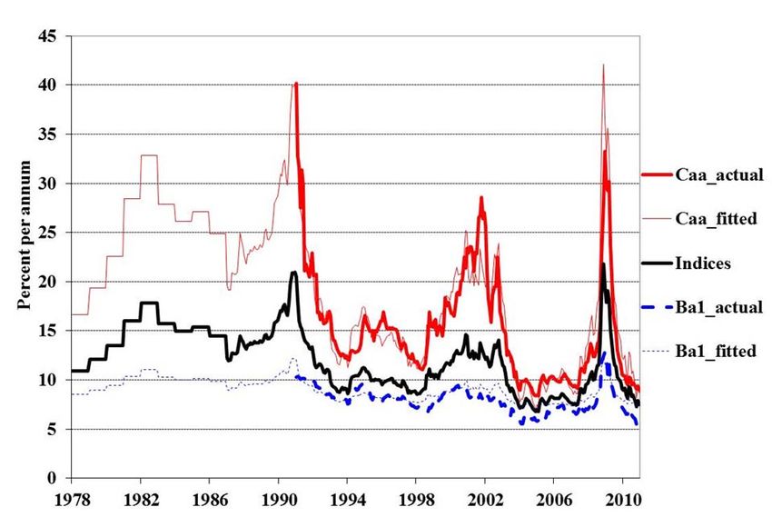
International credit market conditions are controlled for by including the Barclays-
Lehman Brothers index of low grade US corporate spreads24, lagged by one month.
We also take into account credit ratings, by including the residual of a regression of
S&P and Moody’s country credit ratings on the set of other fundamentals and
24
Results are the same when using the 10 year US Treasury yield instead.
17variables in each specification. To capture a country’s political situation we include
the widely used ICRG political risk index25 , lagged by one month, and variables
capturing government changes. Specifically, we include a variable capturing the
number of years in office of the government from the Database of Political
Institutions, and also construct a new government dummy which takes the value of 1
for the first two years after a new administration comes into office. The country fixed
effects will pick up any unobservable and time constant country characteristics,
while year effects account for the potential endogeneity of the timing of restructuring
(e.g. as in countries hurrying to settle with creditors when they anticipate favorable
future borrowing conditions). The definition and sources of variables are listed in
Table 3.
5.4. Results: Haircuts and Subsequent Bond Spreads
Table 4 shows the main results of our bond spread regressions. We start by
replicating the established literature and include a lagged debt crisis dummy as proxy
for sovereign credit history. Like Borensztein and Panizza (2009) we only find
significant effects in the first and second year after the restructuring. The coefficient
of the lagged Ri drops from 260 bp in year one to about 150 bp in year two, but is
clearly insignificant thereafter. Thus, with a binary measure of default, we confirm
the results of the received literature that default effects appear very short-lived.
< Table 4 about here >
The results are notably different when we substitute the restructuring dummy with
our continuous haircut measure, expressed in percentage points (column 2). After
controlling for country and time fixed effects, we find that a one percentage point
increase in haircut is associated with EMBIG spreads that are about 6.75 bp higher in
year one after the restructuring and still about 3.16 bp higher in years four and five.
This means that a haircut of 40%, which is roughly the mean for the EMBIG sample
used here, can be associated with 270 bp higher spreads in year one and 127 basis
25
Results are nearly identical when using the ICRG sub-indicator on government stability.
18points higher in years four and five.26 Accordingly, a one standard deviation increase
in HSZ (about 22 percentage points in this sample) is associated with spreads that are
149 to 70 basis points higher in years one and four and five, respectively. Even when
controlling for ratings (column 3) and/or when including additional macroeconomic
and financial variables, the coefficient of the lagged Hi remains significant up to year
five.
The next columns (4-7) show results for the fully specified model of equation (4),
which includes both the lagged haircut and the lagged restructuring dummies. F-tests
indicate this to be the more complete specification, given that both groups of
variables (the lagged Hi and Ri) are jointly significant. 27 When interpreting the
results, it should be kept in mind that the coefficients of the constitutive terms (here,
the γ coefficients of the lagged Ri) cannot be taken at face value, as they are
conditional on the size of Hi (Brambor et al. 2006). We therefore calculate the
expected mean incremental spread of a restructuring years after its occurrence,
which amounts to Hi+.
The key finding from column (4) is that the lagged values of Hi show high and
significant coefficients up to year seven after the restructuring, although they are
only significant at the 10 percent level in the first three years. The strictest model is
that in column (7), which includes macroeconomic control variables, the ratio of
public debt to GDP, country and year fixed effects and proxies for credit rating and
political risk. In this specification, we find that the incremental spread of a
restructuring, estimated at the mean value of haircuts, is 157 basis points in year 1
but is statistically indistinguishable from zero thereafter. 28 In contrast, we find
significant coefficients for the lagged haircut variables in years four to seven. More
specifically, a one standard deviation increase in haircuts is associated with spreads
that are 112 basis point higher in years four and five, and 161 bp higher in years six
and seven after the restructuring. These are sizable magnitudes, especially when
compared to the findings of earlier studies. For example, the influential early studies
26
The calculation is 40*6.75 = 270 and 40*3.15 = 126.6, respectively.
27
The F-statistic for joint significance of the lagged His in column (4) is 5.46, and it is 4.54 for the
joint significance of the lagged Ris (both with a lower than 1% p-value). Results are similar for
columns (5-7)
28
The calculation is 103.79+1.32*40 = 157.
19by Lindert and Morton (1989) and Özler (1993) and a new paper by Benczur and Ilut
(2009) suggest that past default leads to an average increase in post-crisis spreads of,
at most, 50 basis points. So while defaults may seem costless when estimated at the
mean haircut, larger haircuts can be clearly associated with larger subsequent
spreads.
To validate our findings, section A1.1 in the Appendix provides a large number of
robustness checks. Overall, the results are surprisingly robust with alternative model
specifications or samples, and when controlling for government changes.
6. Haircuts and Duration of Exclusion: Data and Results
To assess the role of haircuts for exclusion duration we construct an annual dataset
on access to capital from 1980 until 2010. The decision to use yearly data is in line
with related research and driven by data availability, because our duration analysis
goes further back in time and spans a larger number of defaulting countries, so that
monthly data are often unavailable. We again focus on access conditions after all 67
final restructurings as defined above, which include all 17 Brady deals as well as all
recent external bond restructurings.
6.1. Dependent Variable: Years of Exclusion
The dependent variable on exclusion duration measures the number of years between
a restructuring event and the successful reaccess to international credit markets.29 To
avoid lengthy discussions on the benefits and drawbacks of alternative definitions
and data sources, we construct a measure of market access that is as comprehensive
as possible and which builds on the two main contributions on this issue in recent
years. Specifically, we combine the approach by Gelos et al. (2011), who focus on
individual syndicated loans and bonds issued in international markets, with the
definition of market access by Richmond and Dias (2009), who use aggregate capital
flows.
29
If a country restructures and regains market access in the same year, we follow the literature in
considering the duration of market exclusion to be one year.
20Our main measure captures “partial” reaccess: it is defined as the first year with an
international loan or bond placement and/or the first year with positive aggregate
credit flows to the public sector. More precisely, the measure takes a value of 1 in
case the country places at least one public or publicly guaranteed bond or syndicated
bank loan on international markets and/or if the public sector receives net transfers
from private foreign creditors. The first criterion builds on primary market issuance
data in international markets from the comprehensive Dealogic database from 1980
until 2010. Specifically, we aggregate information of 8,776 individual public and
publicly guaranteed bonds in 95 developing countries and 10,212 public or publicly
guaranteed syndicated loans from 136 countries.30 In line with Gelos et al. we only
regard issuances that lead to an increase in public sector indebtedness, using debt
stock data to private creditors from the World Bank’s GDF dataset. The second
criterion is constructed from aggregate credit flow data. The dummy is 1 for years in
which bank or bond transfers from foreign private creditors to the public and publicly
guaranteed sector exceed 0. 31 To check the robustness of our findings we also
construct (i) a measure of “full reaccess” defined as the first year in which debt flows
surpass 1% of GDP32, (ii) a measure that focuses on primary market issuance only
(the original Gelos et al. definition), and (iii) a measure that takes into account flows
to the public and private sector of debtor countries (the Richmond and Dias
definition).
6.2. Preliminary Data Analysis
Next, we present descriptive findings on haircut size and the duration of exclusion.
Table A2 in the Appenidx lists the 67 final restructuring events and the respective
30
These samples result from a query retrieving all public and publicly guaranteed emerging market
loans and bonds of developing countries, excluding issues which are placed and marketed in domestic
markets only, according to the Dealogic identifier.
31
Data is available from GDF using the following series: DT.NTR.PBND.CD (net bond transfers) and
DT.NTR.PCBK.CD (net bank transfers). We do not consider arrears as a positive transfer.
32
Specifically, we define full access when (i) bond or loan issuances in international markets exceed
1% of GDP and/or (ii) if net bank and bond transfers to the public sector exceed 1% of GDP. The 1%
threshold is chosen in accordance with Richmond and Dias and represents less than one-half of the
annual public sector borrowing over the entire sample of years and developing countries. GDP data is
taken from the World Development Indicator dataset. The annual volume of loan and bond
placements is again aggregated from Dealogic, while net transfers are from the GDF dataset.
21year of reaccess using various definitions. The average duration from restructuring to
partial reaccess is 5.1 years, while the median is 3 years. We find that exclusion time
increases notably in haircut size. On average, partial reaccess takes just 2.3 years
after cases with HSZ < 30%, while the duration is more than twice as long (6.1 years)
for cases with HSZ >30%. For the full sample, Figure A1 in the Appendix plots the
relationship between HSZ and years until partial reaccess, further pointing to a
positive relationship between the two. The overall picture is similar when using
alternative measures of exclusion duration, such as the one on full reaccess
Another way to illustrate the patterns of exclusion is to plot an empirical survival
function. We apply the non-parametric Kaplan-Meier estimator, which estimates an
unconditional survival function and is very popular in the survival analysis literature,
also because it can take into account censored data. This statistic reports the
compound probability of not having reaccessed the market for each year after the
restructuring. It can be defined as
5
|
where denotes the time at which reaccess occurs for country-case j, 1, … , 67,
are the number of countries that reaccess at time , and is the total number
that have not reaccessed just prior to .
Figure 4 shows the estimated survival function for partial reaccess. Unlike previous
research, we estimate survival functions depending on haircut size of the
restructuring. More specifically, we group cases with HSZ 60% and
those in between. The graph shows that the estimated functions are markedly
different for cases with higher haircuts. More than 60% of countries with HSZ60%. The
figure also shows that exceptionally high haircuts are often followed by
exceptionally long periods of exclusion. Countries imposing HSZ>60% are very likely
to remain excluded even after 10 years, with an unconditional probability exceeding
50%.
226.3. Estimated Model on Exclusion Duration
The univariate analysis shows a correlation between haircut size and exclusion.
However, it is likely that the same factors that are causing the exclusion are also
causing the large haircut in the first place. To address this, we next estimate a semi-
parametric Cox proportional hazard model which allows including constant and
time-varying covariates and can deal with the problems of censored observations and
multiple events.
For this model, the hazard rate for the ith individual (or ith exclusion episode) can be
written as
hi (t ) h0 (t ) exp( zi ), (6)
where h0 (t ) is the baseline hazard function, z a set of covariates and β a vector of
regression coefficients.
The key advantage of the Cox model vis-à-vis other duration models, such as the
parametric Weibull model or the log logistic model, is that it is not necessary to
specify a functional form of the baseline hazard rate h0 (t ) . Instead, the shape of
h0 (t ) is assumed to be unknown and is left unparameterized. Accordingly, we
estimate reduced form models allowing the functional form of the hazard function to
be explained by the data. The model is estimated via a partial likelihood function of
the following form:
i
n exp( z i )
L( ) , (7)
jW ( ti )
exp( z j )
i 1
where W (t i ) ( j : t j t i ) denotes the risk set (i.e. the number of cases that are at risk
of failure) at time ti . The model can be extended in a simple manner once time
varying covariates are included (see Lancaster 1990).
In estimating the model we rely on the variance correction method proposed by Lin
and Wei (1989). This avoids misleading inference in the case of repeated events and
is relevant because some countries in our dataset had multiple restructurings and
23You can also read