9 Projections of Future Climate Change - IPCC
←
→
Page content transcription
If your browser does not render page correctly, please read the page content below
9
Projections of Future Climate Change

Co-ordinating Lead Authors
U. Cubasch, G.A. Meehl

Lead Authors
G.J. Boer, R.J. Stouffer, M. Dix, A. Noda, C.A. Senior, S. Raper, K.S. Yap

Contributing Authors
A. Abe-Ouchi, S. Brinkop, M. Claussen, M. Collins, J. Evans, I. Fischer-Bruns, G. Flato, J.C. Fyfe,
A. Ganopolski, J.M. Gregory, Z.-Z. Hu, F. Joos, T. Knutson, R. Knutti, C. Landsea, L. Mearns, C. Milly,
J.F.B. Mitchell, T. Nozawa, H. Paeth, J. Räisänen, R. Sausen, S. Smith, T. Stocker, A. Timmermann,
U. Ulbrich, A. Weaver, J. Wegner, P. Whetton, T. Wigley, M. Winton, F. Zwiers

Review Editors
J.-W. Kim, J. Stone
Contents

Executive Summary                                         527               9.3.3.1 Implications for temperature of
                                                                                    stabilisation of greenhouse gases     557
9.1   Introduction                                   530              9.3.4 Factors that Contribute to the Response       559
      9.1.1 Background and Recap of Previous Reports 530                    9.3.4.1 Climate sensitivity                   559
      9.1.2 New Types of Model Experiments since                            9.3.4.2 The role of climate sensitivity and
            1995                                     531                            ocean heat uptake                     561
                                                                            9.3.4.3 Thermohaline circulation changes      562
9.2   Climate and Climate Change                          532               9.3.4.4 Time-scales of response               563
      9.2.1 Climate Forcing and Climate Response          532         9.3.5 Changes in Variability                        565
      9.2.2 Simulating Forced Climate Change              534               9.3.5.1 Intra-seasonal variability            566
            9.2.2.1 Signal versus noise                   534               9.3.5.2 Interannual variability               567
            9.2.2.2 Ensembles and averaging               534               9.3.5.3 Decadal and longer time-scale
            9.2.2.3 Multi-model ensembles                 535                       variability                           568
            9.2.2.4 Uncertainty                           536               9.3.5.4 Summary                               570
                                                                      9.3.6 Changes of Extreme Events                     570
9.3   Projections of Climate Change                       536               9.3.6.1 Temperature                           570
      9.3.1 Global Mean Response                          536               9.3.6.2 Precipitation and convection          572
             9.3.1.1 1%/yr CO2 increase (CMIP2)                             9.3.6.3 Extra-tropical storms                 573
                     experiments                          537               9.3.6.4 Tropical cyclones                     574
             9.3.1.2 Projections of future climate from                     9.3.6.5 Commentary on changes in
                     forcing scenario experiments                                   extremes of weather and climate       574
                     (IS92a)                              541               9.3.6.6 Conclusions                           575
             9.3.1.3 Marker scenario experiments
                     (SRES)                               541   9.4   General Summary                                     576
      9.3.2 Patterns of Future Climate Change             543
             9.3.2.1 Summary                              548   Appendix 9.1: Tuning of a Simple Climate Model to
      9.3.3 Range of Temperature Response to SRES               AOGCM Results                                             577
             Emission Scenarios                           554
                                                                References                                                578
Projections of Future Climate Change 527
Executive Summary scaled assuming a value of −0.8 Wm−2 for 1990. Using the IS92
scenarios, the SAR gives a range for the global mean temperature
The results presented in this chapter are based on simulations change for 2100, relative to 1990, of +1 to +3.5°C. The estimated
made with global climate models and apply to spacial scales of range for the six final illustrative SRES scenarios using updated
hundreds of kilometres and larger. Chapter 10 presents results for methods is +1.4 to +5.6°C. The range for the full set of SRES
regional models which operate on smaller spatial scales. Climate scenarios is +1.4 to +5.8°C.
change simulations are assessed for the period 1990 to 2100 and These estimates are larger than in the SAR, partly as a result
are based on a range of scenarios for projected changes in of increases in the radiative forcing, especially the reduced
greenhouse gas concentrations and sulphate aerosol loadings estimated effects of sulphate aerosols in the second half of the
(direct effect). A few Atmosphere-Ocean General Circulation 21st century. By construction, the new range of temperature
Model (AOGCM) simulations include the effects of ozone and/or responses given above includes the climate model response
indirect effects of aerosols (see Table 9.1 for details). Most uncertainty and the uncertainty of the various future scenarios,
integrations1 do not include the less dominant or less well but not the uncertainty associated with the radiative forcings,
understood forcings such as land-use changes, mineral dust, particularly aerosol. Note the AOGCM ranges above are 30-year
black carbon, etc. (see Chapter 6). No AOGCM simulations averages for a period ending at the year 2100 compared to the
include estimates of future changes in solar forcing or in volcanic average for the period 1961 to 1990, while the results for the
aerosol concentrations. simple model are for temperature changes at the year 2100
There are many more AOGCM projections of future climate compared with the year 1990.
available than was the case for the IPCC Second Assessment A traditional measure of climate response is equilibrium
Report (IPCC, 1996) (hereafter SAR). We concentrate on the climate sensitivity derived from 2×CO2 experiments with mixed-
IS92a and draft SRES A2 and B2 scenarios. Some indication of layer models, i.e., Atmospheric General Circulation Models
uncertainty in the projections can be obtained by comparing the (AGCMs) coupled to non-dynamic slab oceans, run to equilib-
responses among models. The range and ensemble standard rium. It has been cited historically to provide a calibration for
deviation are used as a measure of uncertainty in modelled models used in climate change experiments. The mean and
response. The simulations are a combination of a forced climate standard deviation of this quantity from seventeen mixed-layer
change component together with internally generated natural models used in the SAR are +3.8 and +0.8°C, respectively. The
variability. A number of modelling groups have produced same quantities from fifteen models in active use are +3.5 and
ensembles of simulations where the projected forcing is the same +0.9°C, not significantly different from the values in the SAR.
but where variations in initial conditions result in different These quantities are model dependent, and the previous estimated
evolutions of the natural variability. Averaging these integrations range for this quantity, widely cited as +1.5 to +4.5°C, still
preserves the forced climate change signal while averaging out the encompasses the more recent model sensitivity estimates.
natural variability noise, and so gives a better estimate of the A more relevant measure of transient climate change is the
models’ projected climate change. transient climate response (TCR). It is defined as the globally
For the AOGCM experiments, the mean change and the averaged surface air temperature change for AOGCMs at the time
range in global average surface air temperature (SAT) for the of CO2 doubling in 1%/yr CO2 increase experiments. The TCR
1961 to 1990 average to the mid-21st century (2021 to 2050) for combines elements of model sensitivity and factors that affect
IS92a is +1.3°C with a range from +0.8 to +1.7°C for greenhouse response (e.g., ocean heat uptake). It provides a useful measure
gas plus sulphates (GS) as opposed to +1.6°C with a range from for understanding climate system response and allows direct
+1.0 to +2.1°C for greenhouse gas only (G). For SRES A2 the comparison of global coupled models. The range of TCR for
mean is +1.1°C with a range from +0.5 to +1.4°C, and for B2, the current AOGCMs is +1.1 to +3.1°C with an average of 1.8°C.
mean is +1.2°C with a range from +0.5 to +1.7°C. The 1%/yr CO2 increase represents the changes in radiative
For the end of the 21st century (2071 to 2100), for the draft forcing due to all greenhouse gases, hence this is a higher rate
SRES marker scenario A2, the global average SAT change from than is projected for CO2 alone. This increase of radiative forcing
AOGCMs compared with 1961 to 1990 is +3.0°C and the range lies on the high side of the SRES scenarios (note also that CO2
is +1.3 to +4.5°C, and for B2 the mean SAT change is +2.2°C and doubles around mid-21st century in most of the scenarios).
the range is +0.9 to +3.4°C. However these experiments are valuable for promoting the
AOGCMs can only be integrated for a limited number of understanding of differences in the model responses.
scenarios due to computational expense. Therefore, a simple The following findings from the models analysed in this
climate model is used here for the projections of climate change chapter corroborate results from the SAR (projections of regional
for the next century. The simple model is tuned to simulate the climate change are given in Chapter 10) for all scenarios consid-
response found in several of the AOGCMs used here. The ered. We assign these to be virtually certain to very likely
forcings for the simple model are based on the radiative forcing (defined as agreement among most models, or, where only a
estimates from Chapter 6, and are slightly different to the small number of models have been analysed and their results are
forcings used by the AOGCMs. The indirect aerosol forcing is physically plausible, these have been assessed to characterise
those from a larger number of models). The more recent results
1 In this report, the term “integration” is used to mean a climate model are generally obtained from models with improved parametriza-
rum. tions (e.g., better land-surface process schemes).528 Projections of Future Climate Change
• The troposphere warms, stratosphere cools, and near surface • The deep ocean has a very long thermodynamic response time
temperature warms. to any changes in radiative forcing; over the next century, heat
anomalies penetrate to depth mainly at high latitudes where
• Generally, the land warms faster than the ocean, the land mixing is greatest.
warms more than the ocean after forcing stabilises, and there is
greater relative warming at high latitudes. A second category of results assessed here are those that are new
since the SAR, and we ascribe these to be very likely (as defined
• The cooling effect of tropospheric aerosols moderates warming above):
both globally and locally, which mitigates the increase in SAT.
• The range of the TCR is limited by the compensation between
• The SAT increase is smaller in the North Atlantic and circum- the effective climate sensitivity (ECS) and ocean heat uptake.
polar Southern Ocean regions relative to the global mean. For instance, a large ECS, implying a large temperature
change, is offset by a comparatively large heat flux into the
• As the climate warms, Northern Hemisphere snow cover and ocean.
sea-ice extent decrease.
• Including the direct effect of sulphate aerosols (IS92a or
• The globally averaged mean water vapour, evaporation and similar) reduces global mean mid-21st century warming
precipitation increase. (though there are uncertainties involved with sulphate aerosol
forcing – see Chapter 6).
• Most tropical areas have increased mean precipitation, most of
the sub-tropical areas have decreased mean precipitation, and • Projections of climate for the next 100 years have a large range
in the high latitudes the mean precipitation increases. due both to the differences of model responses and the range of
emission scenarios. Choice of model makes a difference
• Intensity of rainfall events increases. comparable to choice of scenario considered here.
• There is a general drying of the mid-continental areas during • In experiments where the atmospheric greenhouse gas concen-
summer (decreases in soil moisture). This is ascribed to a tration is stabilised at twice its present day value, the North
combination of increased temperature and potential evapora- Atlantic THC recovers from initial weakening within one to
tion that is not balanced by increases in precipitation. several centuries.
• A majority of models show a mean El Niño-like response in the • The increases in surface air temperature and surface absolute
tropical Pacific, with the central and eastern equatorial Pacific humidity result in even larger increases in the heat index (a
sea surface temperatures warming more than the western measure of the combined effects of temperature and moisture).
equatorial Pacific, with a corresponding mean eastward shift of The increases in surface air temperature also result in an
precipitation. increase in the annual cooling degree days and a decrease in
heating degree days.
• Available studies indicate enhanced interannual variability of
northern summer monsoon precipitation. Additional new results since the SAR; these are assessed to be
likely due to many (but not most) models showing a given result,
• With an increase in the mean surface air temperature, there or a small number of models showing a physically plausible
are more frequent extreme high maximum temperatures and result.
less frequent extreme low minimum temperatures. There is a
decrease in diurnal temperature range in many areas, with • Areas of increased 20 year return values of daily maximum
night-time lows increasing more than daytime highs. A temperature events are largest mainly in areas where soil
number of models show a general decrease in daily variability moisture decreases; increases in return values of daily
of surface air temperature in winter, and increased daily minimum temperature especially occur over most land areas
variability in summer in the Northern Hemisphere land areas. and are generally larger where snow and sea ice retreat.
• The multi-model ensemble signal to noise ratio is greater for • Precipitation extremes increase more than does the mean and
surface air temperature than for precipitation. the return period for extreme precipitation events decreases
almost everywhere.
• Most models show weakening of the Northern Hemisphere
thermohaline circulation (THC), which contributes to a Another category includes results from a limited number of
reduction in the surface warming in the northern North studies which are new, less certain, or unresolved, and we assess
Atlantic. Even in models where the THC weakens, there is still these to have medium likelihood, though they remain physically
a warming over Europe due to increased greenhouse gases. plausible:Projections of Future Climate Change 529
• Although the North Atlantic THC weakens in most models, the that show increases, this is related to an increase in thermocline
relative roles of surface heat and freshwater fluxes vary from intensity, but other models show no significant change and
model to model. Wind stress changes appear to play only a there are considerable uncertainties due to model limitations of
minor role. simulating ENSO in the current generation of AOGCMs
(Chapter 8).
• It appears that a collapse in the THC by the year 2100 is less
likely than previously discussed in the SAR, based on the • Several models produce less of the weak but more of the deeper
AOGCM results to date. mid-latitude lows, meaning a reduced total number of storms.
Techniques are being pioneered to study the mechanisms of the
• Beyond 2100, the THC could completely shut-down, possibly changes and of variability, but general agreement among
irreversibly, in either hemisphere if the rate of change of models has not been reached.
radiative forcing was large enough and applied long enough.
The implications of a complete shut-down of the THC have not • There is some evidence that shows only small changes in the
been fully explored. frequency of tropical cyclones derived from large-scale
parameters related to tropical cyclone genesis, though some
• Although many models show an El Niño-like change in the mean measures of intensities show increases, and some theoretical
state of tropical Pacific SSTs, the cause is uncertain. It has been and modelling studies suggest that upper limit intensities could
related to changes in the cloud radiative forcing and/or evapora- increase (for further discussion see Chapter 10).
tive damping of the east-west SST gradient in some models.
• There is no clear agreement concerning the changes in
• Future changes in El Niño-Southern Oscillation (ENSO) frequency or structure of naturally occurring modes of
interannual variability differ from model to model. In models variability such as the North Atlantic Oscillation.530 Projections of Future Climate Change
9.1 Introduction whereby the fluxes of heat, fresh water and momentum were
either singly or in some combination adjusted at the air-sea
The purpose of this chapter is to assess and quantify projections interface to account for incompatibilities in the component
of possible future climate change from climate models. A models. However, the assessment of those models suggested that
background of concepts used to assess climate change experi- the main results concerning the patterns and magnitudes of the
ments is presented in Section 9.2, followed by Section 9.3 which climate changes in the model without flux adjustment were
includes results from ensembles of several categories of future essentially the same as in the flux-adjusted models.
climate change experiments, factors that contribute to the The most recent IPCC Second Assessment Report (IPCC,
response of those models, changes in variability and changes in 1996) (hereafter SAR) included a much more extensive collec-
extremes. Section 9.4 is a synthesis of our assessment of model tion of global coupled climate model results from models run
projections of climate change. with what became a standard 1%/yr CO2-increase experiment.
In a departure from the organisation of the SAR, the assess- These models corroborated the results in the earlier assessment
ment of regional information derived in some way from global regarding the time evolution of warming and the reduced
models (including results from embedded regional high resolu- warming in regions of deep ocean mixing. There were additional
tion models, downscaling, etc.) now appears in Chapter 10. studies of changes in variability in the models in addition to
changes in the mean, and there were more results concerning
9.1.1 Background and Recap of Previous Reports possible changes in climate extremes. Information on possible
future changes of regional climate was included as well.
Studies of projections of future climate change use a hierarchy of The SAR also included results from the first two global
coupled ocean/atmosphere/sea-ice/land-surface models to coupled models run with a combination of increasing CO2 and
provide indicators of global response as well as possible regional sulphate aerosols for the 20th and 21st centuries. Thus, for the
patterns of climate change. One type of configuration in this first time, models were run with a more realistic forcing history
climate model hierarchy is an Atmospheric General Circulation for the 20th century and allowed the direct comparison of the
Model (AGCM), with equations describing the time evolution of model’s response to the observations. The combination of the
temperature, winds, precipitation, water vapour and pressure, warming effects on a global scale from increasing CO2 and the
coupled to a simple non-dynamic “slab” upper ocean, a layer of regional cooling from the direct effect of sulphate aerosols
water usually around 50 m thick that calculates only temperature produced a better agreement with observations of the time
(sometimes referred to as a “mixed-layer model”). Such air-sea evolution of the globally averaged warming and the patterns of
coupling allows those models to include a seasonal cycle of solar 20th century climate change. Subsequent experiments have
radiation. The sea surface temperatures (SSTs) respond to attempted to quantify and include additional forcings for 20th
increases in carbon dioxide (CO2), but there is no ocean century climate (Chapter 8), with projected outcomes for those
dynamical response to the changing climate. Since the full depth forcings in scenario integrations into the 21st century discussed
of the ocean is not included, computing requirements are below.
relatively modest so these models can be run to equilibrium with In the SAR, the two global coupled model runs with the
a doubling of atmospheric CO2. This model design was prevalent combination of CO2 and direct effect of sulphate aerosols both
through the 1980s, and results from such equilibrium simulations gave a warming at mid-21st century relative to 1990 of around
were an early basis of societal concern about the consequences of 1.5°C. To investigate more fully the range of forcing scenarios
increasing CO2. and uncertainty in climate sensitivity (defined as equilibrium
However, such equilibrium (steady-state) experiments globally averaged surface air temperature increase due to a
provide no information on time-dependent climate change and no doubling of CO2, see discussion in Section 9.2 below) a simpler
information on rates of climate change. In the late 1980s, more climate model was used. Combining low emissions with low
comprehensive fully coupled global ocean/atmosphere/sea- sensitivity and high emissions with high sensitivity gave an
ice/land-surface climate models (also referred to as Atmosphere- extreme range of 1 to 4.5°C for the warming in the simple model
Ocean Global Climate Models, Atmosphere-Ocean General at the year 2100 (assuming aerosol concentrations constant at
Circulation Models or simply AOGCMs) began to be run with 1990-levels). These projections were generally lower than
slowly increasing CO2, and preliminary results from two such corresponding projections in IPCC (1990) because of the
models appeared in the 1990 IPCC Assessment (IPCC, 1990). inclusion of aerosols in the pre-1990 radiative forcing history.
In the 1992 IPCC update prior to the Earth Summit in Rio When the possible effects of future changes of anthropogenic
de Janeiro (IPCC, 1992), there were results from four AOGCMs aerosol as prescribed in the IS92 scenarios were incorporated this
run with CO2 increasing at 1%/yr to doubling around year 70 of led to lower projections of temperature change of between 1°C
the simulations (these were standardised sensitivity experiments, and 3.5°C with the simple model.
and consequently no actual dates were attached). Inclusion of Spatial patterns of climate change simulated by the global
the full ocean meant that warming at high latitudes was not as coupled models in the SAR corroborated the IPCC (1990)
uniform as from the non-dynamic mixed-layer models. In results. With increasing greenhouse gases the land was projected
regions of deep ocean mixing in the North Atlantic and Southern to warm generally more than the oceans, with a maximum annual
Oceans, warming was less than at other high latitude locations. mean warming in high latitudes associated with reduced snow
Three of those four models used some form of flux adjustment cover and increased runoff in winter, with greatest warming atProjections of Future Climate Change 531
high northern latitudes. Including the effects of aerosols led to a integrations continue for several hundred years in order to study
somewhat reduced warming in middle latitudes of the Northern the commitment to climate change. The 1%/yr rate of increase for
Hemisphere and the maximum warming in northern high future climate, although larger than actual CO2 increase observed
latitudes was less extensive since most sulphate aerosols are to date, is meant to account for the radiative effects of CO2 and
produced in the Northern Hemisphere. All models produced an other trace gases in the future and is often referred to as “equiva-
increase in global mean precipitation but at that time there was lent CO2” (see discussion in Section 9.2.1). This rate of increase
little agreement among models on changes in storminess in a in radiative forcing is often used in model intercomparison studies
warmer world and conclusions regarding extreme storm events to assess general features of model response to such forcing.
were even more uncertain. In 1996, the IPCC began the development of a new set of
emissions scenarios, effectively to update and replace the well-
known IS92 scenarios. The approved new set of scenarios is
9.1.2 New Types of Model Experiments since 1995
described in the IPCC Special Report on Emission Scenarios
The progression of experiments including additional forcings has (SRES) (Nakićenović et al., 2000; see more complete discussion of
continued and new experiments with additional greenhouse gases SRES scenarios and forcing in Chapters 3, 4, 5 and 6). Four
(such as ozone, CFCs, etc., as well as CO2) will be assessed in different narrative storylines were developed to describe consis-
this chapter. tently the relationships between emission driving forces and their
In contrast to the two global coupled climate models in the evolution and to add context for the scenario quantification (see
1990 Assessment, the Coupled Model Intercomparison Project Box 9.1). The resulting set of forty scenarios (thirty-five of which
(CMIP) (Meehl et al., 2000a) includes output from about twenty contain data on the full range of gases required for climate
AOGCMs worldwide, with roughly half of them using flux adjust- modelling) cover a wide range of the main demographic, economic
ment. Nineteen of them have been used to perform idealised 1%/yr and technological driving forces of future greenhouse gas and
CO2-increase climate change experiments suitable for direct sulphur emissions. Each scenario represents a specific quantifica-
intercomparison and these are analysed here. Roughly half that tion of one of the four storylines. All the scenarios based on the
number have also been used in more detailed scenario experiments same storyline constitute a scenario “family”. (See Box 9.1, which
with time evolutions of forcings including at least CO2 and sulphate briefly describes the main characteristics of the four SRES
aerosols for 20th and 21st century climate. Since there are some storylines and scenario families.) The SRES scenarios do not
differences in the climate changes simulated by various models include additional climate initiatives, which means that no
even if the same forcing scenario is used, the models are compared scenarios are included that explicitly assume implementation of the
to assess the uncertainties in the responses. The comparison of 20th UNFCCC or the emissions targets of the Kyoto Protocol. However,
century climate simulations with observations (see Chapter 8) has greenhouse gas emissions are directly affected by non-climate
given us more confidence in the abilities of the models to simulate change policies designed for a wide range of other purposes.
possible future climate changes in the 21st century and reduced the Furthermore, government policies can, to varying degrees,
uncertainty in the model projections (see Chapter 14). The newer influence the greenhouse gas emission drivers and this influence is
model integrations without flux adjustment give us indications of broadly reflected in the storylines and resulting scenarios.
how far we have come in removing biases in the model Because SRES was not approved until 15 March 2000, it was
components. The results from CMIP confirm what was noted in the too late for the modelling community to incorporate the scenarios
SAR in that the basic patterns of climate system response to external into their models and have the results available in time for this Third
forcing are relatively robust in models with and without flux adjust- Assessment Report. Therefore, in accordance with a decision of the
ment (Gregory and Mitchell, 1997; Fanning and Weaver, 1997; IPCC Bureau in 1998 to release draft scenarios to climate modellers
Meehl et al., 2000a). This also gives us more confidence in the (for their input to the Third Assessment Report) one marker
results from the models still using flux adjustment. scenario was chosen from each of four of the scenario groups based
The IPCC data distribution centre (DDC) has collected on the storylines (A1B, A2, B1 and B2) (Box 9.1). The choice of
results from a number of transient scenario experiments. They the markers was based on which initial quantification best reflected
start at an early time of industrialisation and most have been run the storyline, and features of specific models. Marker scenarios are
with and without the inclusion of the direct effect of sulphate no more or less likely than any other scenarios but these scenarios
aerosols. Note that most models do not use other forcings have received the closest scrutiny. Scenarios were also selected
described in Chapter 6 such as soot, the indirect effect of sulphate later to illustrate the other two scenario groups (A1FI and A1T),
aerosols, or land-use changes. Forcing estimates for the direct hence there is an illustrative scenario for each of the six scenario
effect of sulphate aerosols and other trace gases included in the groups. These latter two illustrative scenarios were not selected in
DDC models are given in Chapter 6. Several models also include time for AOGCM models to utilise them in this report. In fact,
effects of tropospheric and stratospheric ozone changes. time and computer resource limitations dictated that most
Additionally, multi-member ensemble integrations have been modelling groups could run only A2 and B2, and results from
run with single models with the same forcing. So-called “stabili- those integrations are evaluated in this chapter. However, results
sation” experiments have also been run with the atmospheric for all six illustrative scenarios are shown here using a simple
greenhouse gas concentrations increasing by 1%/yr or following climate model discussed below. The IS92a scenario is also used in
an IPCC scenario, until CO2-doubling, tripling or quadrupling. a number of the results presented in this chapter in order to
The greenhouse gas concentration is then kept fixed and the model provide direct comparison with the results in the SAR.532 Projections of Future Climate Change
Box 9.1: The Emissions Scenarios of the Special Report on Emissions Scenarios (SRES)
A1. The A1 storyline and scenario family describe a future world of very rapid economic growth, global population that peaks in
mid-century and declines thereafter, and the rapid introduction of new and more efficient technologies. Major underlying themes are
convergence among regions, capacity building and increased cultural and social interactions, with a substantial reduction in regional
differences in per capita income. The A1 scenario family develops into three groups that describe alternative directions of techno-
logical change in the energy system. The three A1 groups are distinguished by their technological emphasis: fossil intensive (A1FI),
non-fossil energy sources (A1T), or a balance across all sources (A1B) (where balanced is defined as not relying too heavily on one
particular energy source, on the assumption that similar improvement rates apply to all energy supply and end use technologies).
A2. The A2 storyline and scenario family describe a very heterogeneous world. The underlying theme is self-reliance and preser-
vation of local identities. Fertility patterns across regions converge very slowly, which results in continuously increasing popula-
tion. Economic development is primarily regionally oriented and per capita economic growth and technological change are more
fragmented and slower than in other storylines.
B1. The B1 storyline and scenario family describe a convergent world with the same global population, that peaks in mid-century
and declines thereafter, as in the A1 storyline, but with rapid change in economic structures toward a service and information
economy, with reductions in material intensity and the introduction of clean and resource-efficient technologies. The emphasis is
on global solutions to economic, social and environmental sustainability, including improved equity, but without additional climate
initiatives.
B2. The B2 storyline and scenario family describe a world in which the emphasis is on local solutions to economic, social and
environmental sustainability. It is a world with continuously increasing global population, at a rate lower than A2, intermediate
levels of economic development, and less rapid and more diverse technological change than in the B1 and A1 storylines. While the
scenario is also oriented towards environmental protection and social equity, it focuses on local and regional levels.
The final four marker scenarios contained in SRES differ in governing the climate system as represented in the models. The
minor ways from the draft scenarios used for the AOGCM simulated climate change depends, therefore, on projected
experiments described in this report. In order to ascertain the changes in emissions, the changes in atmospheric greenhouse gas
likely effect of differences in the draft and final SRES scenarios and particulate (aerosol) concentrations that result, and the
each of the four draft and final marker scenarios were studied manner in which the models respond to these changes. The
using a simple climate model tuned to the AOGCMs used in this response of the climate system to a given change in forcing is
report. For three of the four marker scenarios (A1B, A2 and B2) broadly characterised by its “climate sensitivity”. Since the
temperature change from the draft and final scenarios are very climate system requires many years to come into equilibrium
similar. The primary difference is a change to the standardised with a change in forcing, there remains a “commitment” to
values for 1990 to 2000, which is common to all these scenarios. further climate change even if the forcing itself ceases to change.
This results in a higher forcing early in the period. There are Observations of the climate system and the output of models
further small differences in net forcing, but these decrease until, are a combination of a forced climate change “signal” and
by 2100, differences in temperature change in the two versions of internally generated natural variability which, because it is
these scenarios are in the range 1 to 2%. For the B1 scenario, random and unpredictable on long climate time-scales, is charac-
however, temperature change is significantly lower in the final terised as climate “noise”. The availability of multiple simula-
version, leading to a difference in the temperature change in 2100 tions from a given model with the same forcing, and of simula-
of almost 20%, as a result of generally lower emissions across the tions from many models with similar forcing, allows ensemble
full range of greenhouse gases. For descriptions of the simula- methods to be used to better characterise projected climate
tions, see Section 9.3.1. change and the agreement or disagreement (a measure of
reliability) of model results.
9.2 Climate and Climate Change
9.2.1 Climate Forcing and Climate Response
Chapter 1 discusses the nature of the climate system and the
climate variability and change it may undergo, both naturally and The heat balance
as a consequence of human activity. The projections of future Broad aspects of global mean temperature change may be
climate change discussed in this chapter are obtained using illustrated using a simple representation of the heat budget of the
climate models in which changes in atmospheric composition are climate system expressed as:
specified. The models “translate” these changes in composition
dH/dt = F − αT.
into changes in climate based on the physical processesProjections of Future Climate Change 533
Here F is the radiative forcing change as discussed in Chapter 6; forcing change (e.g., in the SAR and the CMIP2 intercomparison).
αT represents the net effect of processes acting to counteract The resulting information is also used to calibrate simpler models
changes in mean surface temperature, and dH/dt is the rate of heat which may then be employed to investigate a broad range of
storage in the system. All terms are differences from unperturbed forcing scenarios as is done in Section 9.3.3. Figure 9.1 illustrates
equilibrium climate values. A positive forcing will act to increase the global mean temperature evolution for this standardised
the surface temperature and the magnitude of the resulting forcing in a simple illustrative example with no exchange with the
increase will depend on the strength of the feedbacks measured by deep ocean (the green curves) and for a full coupled AOGCM (the
αΤ. If α is large, the temperature change needed to balance a red curves). The diagram also illustrates the transient climate
given change in forcing is small and vice versa. The result will response, climate sensitivity and warming commitment.
also depend on the rate of heat storage which is dominated by the
ocean so that dH/dt = dHo/dt = Fo where Ho is the ocean heat TCR − Transient climate response
content and Fo is the flux of heat into the ocean. With this approx- The temperature change at any time during a climate change
imation the heat budget becomes F = αT + Fo, indicating that both integration depends on the competing effects of all of the
the feedback term and the flux into the ocean act to balance the processes that affect energy input, output, and storage in the
radiative forcing for non-equilibrium conditions. ocean. In particular, the global mean temperature change which
occurs at the time of CO2 doubling for the specific case of a 1%/yr
Radiative forcing in climate models increase of CO2 is termed the “transient climate response” (TCR)
A radiative forcing change, symbolised by F above, can result of the system. This temperature change, indicated in Figure 9.1,
from changes in greenhouse gas concentrations and aerosol integrates all processes operating in the system, including the
loading in the atmosphere. The calculation of F is discussed in strength of the feedbacks and the rate of heat storage in the ocean,
Chapter 6 where a new estimate of CO2 radiative forcing is given to give a straightforward measure of model response to a change
which is smaller than the value in the SAR. According to Section in forcing. The range of TCR values serves to illustrate and
6.3.1, the lower value is due mainly to the fact that stratospheric calibrate differences in model response to the same standardised
temperature adjustment was not included in the (previous) forcing. Analogous TCR measures may be used, and compared
estimates given for the forcing change. It is important to note that among models, for other forcing scenarios.
this new radiative forcing estimate does not affect the climate
change and equilibrium climate sensitivity calculations made with Equilibrium climate sensitivity
general circulation models. The effect of a change in greenhouse The “equilibrium climate sensitivity” (IPCC 1990, 1996) is
gas concentration and/or aerosol loading in a general circulation defined as the change in global mean temperature, T2x , that results
model (GCM) is calculated internally and interactively based on, when the climate system, or a climate model, attains a new
and in turn affecting, the three dimensional state of the equilibrium with the forcing change F2x resulting from a doubling
atmosphere. In particular, the stratospheric temperature responds of the atmospheric CO2 concentration. For this new equilibrium
to changes in radiative fluxes due to changes in CO2 concentration dH/dt = 0 in the simple heat budget equation and F2x = αT2x
and the GCM calculation includes this effect. indicating a balance between energy input and output. The
equilibrium climate sensitivity
Equivalent CO2 T2x = F2x / α
The radiative effects of the major greenhouse gases which are
well-mixed throughout the atmosphere are often represented in is inversely proportional to α, which measures the strength of the
GCMs by an “equivalent” CO2 concentration, namely the CO2 feedback processes in the system that act to counter a change in
concentration that gives a radiative forcing equal to the sum of the forcing. The equilibrium climate sensitivity is a straightforward,
forcings for the individual greenhouse gases. When used in although averaged, measure of how the system responds to a
simulations of forced climate change, the increase in “equivalent specific forcing change and may be used to compare model
CO2” will be larger than that of CO2 by itself, since it also responses, calibrate simple climate models, and to scale tempera-
accounts for the radiative effects of other gases. ture changes in other circumstances.
In earlier assessments, the climate sensitivity was obtained
1%/yr increasing CO2 from calculations made with AGCMs coupled to mixed-layer
A common standardised forcing scenario specifies atmospheric upper ocean models (referred to as mixed-layer models). In that
CO2 to increase at a rate of 1%/year compound until the concen- case there is no exchange of heat with the deep ocean and a model
tration doubles (or quadruples) and is then held constant. The CO2 can be integrated to a new equilibrium in a few tens of years. For a
content of the atmosphere has not, and likely will not, increase at full coupled atmosphere/ocean GCM, however, the heat exchange
this rate (let alone suddenly remain constant at twice or four times with the deep ocean delays equilibration and several millennia,
an initial value). If regarded as a proxy for all greenhouse gases, rather than several decades, are required to attain it. This difference
however, an “equivalent CO2” increase of 1%/yr does give a is illustrated in Figure 9.1 where the smooth green curve illustrates
forcing within the range of the SRES scenarios. the rapid approach to a new climate equilibrium in an idealised
This forcing prescription is used to illustrate and to quantify mixed-layer case while the red curve is the result of a coupled
aspects of AOGCM behaviour and provides the basis for the model integration and indicates the much longer time needed to
analysis and intercomparison of modelled responses to a specified attain equilibrium when there is interaction with the deep ocean.534 Projections of Future Climate Change
increase that has already been experienced, that will occur before
time of CO2 the system reaches a new equilibrium with radiative forcing
quadrupling stabilised at the current value. This behaviour is illustrated in
Figure 9.1 for the idealised case of instantaneous stabilisation at
2× and 4×CO2 . Analogous behaviour would be seen for more
realistic stabilisation scenarios.
additional warming
Temperature change (°C)
commitment:forcing
stabilized at 4×CO2 9.2.2 Simulating Forced Climate Change
9.2.2.1 Signal versus noise
A climate change simulation produces a time evolving three
dimensional distribution of temperature and other climate
variables. For the real system or for a model, and taking temper-
additional warming
commitment: forcing
ature as an example, this is expressed as T = T0 + T0' for pre-
TCR transient climate T2x
response stabilized at 2×CO2 industrial equilibrium conditions. T is now the full temperature
field rather than the global mean temperature change of Section
3.5°C climate sensitivity
9.2.1. T0 represents the temperature structure of the mean
time of CO2 climate, which is determined by the (pre-industrial) forcing, and
doubling 1%/year CO2 increase
T0' the internally generated random natural variability with zero
stabilization at 2× and 4×CO2
mean. For climate which is changing as a consequence of
0 50 100 150 200 250 300 350 400 450 500 increasing atmospheric greenhouse gas concentrations or other
Year
forcing changes, T = T0 + Tf + T' where Tf is the deterministic
Figure 9.1: Global mean temperature change for 1%/yr CO2 increase climate change caused by the changing forcing, and T' is the
with subsequent stabilisation at 2×CO2 and 4×CO2. The red curves are natural variability under these changing conditions. Changes in
from a coupled AOGCM simulation (GFDL_R15_a) while the green the statistics of the natural variability, that is in the statistics of T0'
curves are from a simple illustrative model with no exchange of energy vs T', are of considerable interest and are discussed in Sections
with the deep ocean. The “transient climate response”, TCR, is the 9.3.5 and 9.3.6 which treat changes in variability and extremes.
temperature change at the time of CO2 doubling and the “equilibrium The difference in temperature between the control and
climate sensitivity”, T2x, is the temperature change after the system has climate change simulations is written as ∆T = Tf + (T' − T0') = Tf
reached a new equilibrium for doubled CO2, i.e., after the “additional
+ T'', and is a combination of the deterministic signal Tf and a
warming commitment” has been realised.
random component T'' = T' − T0' which has contributions from
the natural variability of both simulations. A similar expression
Effective climate sensitivity arises when calculating climate change as the difference between
Although the definition of equilibrium climate sensitivity is an earlier and a later period in the observations or a simulation.
straightforward, it applies to the special case of equilibrium Observed and simulated climate change are the sum of the forced
climate change for doubled CO2 and requires very long simula- “signal” and the natural variability “noise” and it is important to
tions to evaluate with a coupled model. The “effective climate be able to separate the two. The natural variability that obscures
sensitivity” is a related measure that circumvents this require- the forced signal may be at least partially reduced by averaging.
ment. The inverse of the feedback term α is evaluated from model
output for evolving non-equilibrium conditions as 9.2.2.2 Ensembles and averaging
An ensemble consists of a number of simulations undertaken
1/ αe = T / (F − dHo/dt) = T / (F − Fo)
with the same forcing scenario, so that the forced change Tf is
and the effective climate sensitivity is calculated as the same for each, but where small perturbations to remote
initial conditions result in internally generated climate
Te = F2x / αe
variability that is different for each ensemble member. Small
with units and magnitudes directly comparable to the equilibrium ensembles of simulations have been performed with a number
sensitivity. The effective sensitivity becomes the equilibrium of models as indicated in the “number of simulations” column
sensitivity under equilibrium conditions with 2×CO2 forcing. The in Table 9.1. Averaging over the ensemble of results, indicated
effective climate sensitivity is a measure of the strength of the by braces, gives the ensemble mean climate change as {∆T} =
feedbacks at a particular time and it may vary with forcing Tf + {T''}. For independent realisations, the natural variability
history and climate state. noise is reduced by the ensemble averaging (averaging to zero
for a large enough ensemble) so that {∆T} is an improved
Warming commitment estimate of the model’s forced climate change Tf. This is
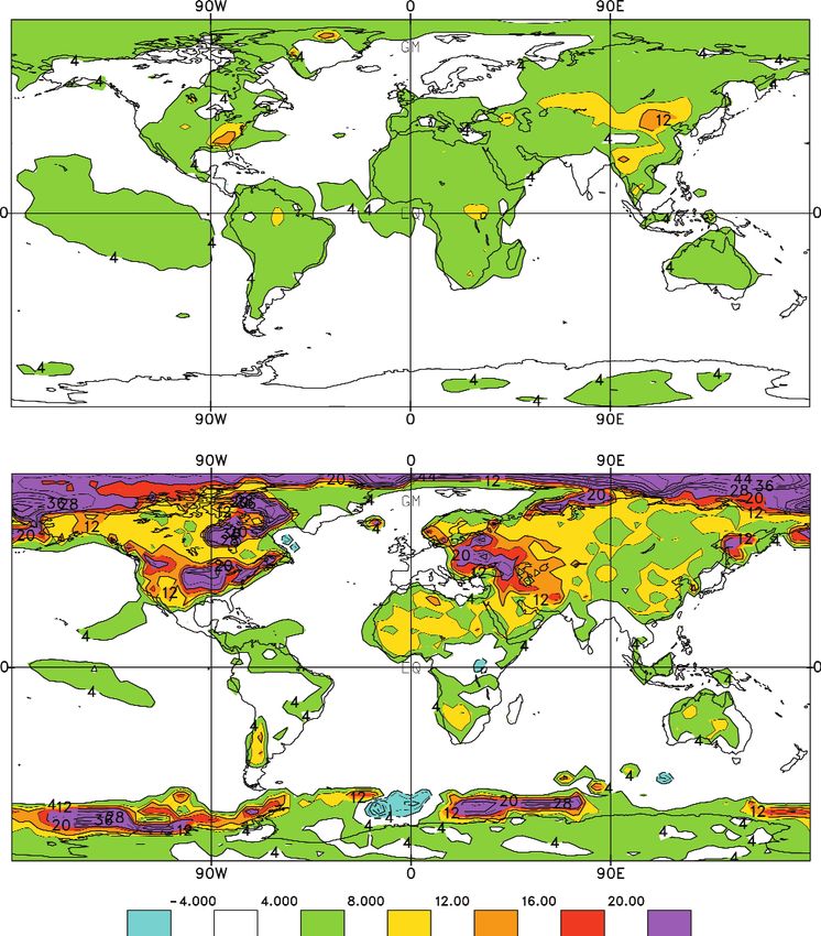
An increase in forcing implies a “commitment” to future illustrated in Figure 9.2, which shows the simulated temperature
warming even if the forcing stops increasing and is held at a differences from 1975 to 1995 to the first decade in the 21st
constant value. At any time, the “additional warming commit- century for three climate change simulations made with the
ment” is the further increase in temperature, over and above the same model and the same forcing scenario but starting fromProjections of Future Climate Change 535
1 2
3 ENSEMBLE MEAN
- 3.0 - 2.0 - 1.0 - 0.5 0 0.5 1.0 2.0 3.0
Figure 9.2: Three realisations of the geographical distribution of temperature differences from 1975 to 1995 to the first decade in the 21st century
made with the same model (CCCma CGCM1) and the same IS92a greenhouse gas and aerosol forcing but with slightly different initial conditions
a century earlier. The ensemble mean is the average of the three realisations. (Unit: oC).
slightly different initial conditions more than a century earlier. 9.2.2.3 Multi-model ensembles
The differences between the simulations reflect differences in The collection of coupled climate model results that is available
the natural variability. The ensemble average over the three for this report permits a multi-model ensemble approach to the
realisations, also shown in the diagram, is an estimate of the synthesis of projected climate change. Multi-model ensemble
model’s forced climate change where some of this natural approaches are already used in short-range climate forecasting
variability has been averaged out. (e.g., Graham et al., 1999; Krishnamurti et al., 1999; Brankovic
The ensemble variance for a particular model, assuming and Palmer, 2000; Doblas-Reyes et al., 2000; Derome et al.,
there is no correlation between the forced component and the 2001). When applied to climate change, each model in the
variability, is σ2∆T = {(∆T − {∆T})2} = {(T'' − {T''})2} = σ2N ensemble produces a somewhat different projection and, if these
which gives a measure of the natural variability noise. The represent plausible solutions to the governing equations, they
“signal to noise ratio”, {∆T}/ σ∆T , compares the strength of the may be considered as different realisations of the climate change
climate change signal to this natural variability noise. The signal drawn from the set of models in active use and produced with
stands out against the noise when and where this ratio is large. current climate knowledge. In this case, temperature is
The signal will be better represented by the ensemble mean as represented as T = T0 + TF + Tm + T' where TF is the determin-
the size of the ensemble grows and the noise is averaged out istic forced climate change for the real system and Tm= Tf −TF is
over more independent realisations. This is indicated by the the error in the model’s simulation of this forced response. T' now
width, {∆T} ± 2σ∆T /√n, of the approximate 95% confidence also includes errors in the statistical behaviour of the simulated
interval which decreases as the ensemble size n increases. natural variability. The multi-model ensemble mean estimate of
The natural variability may be further reduced by averaging forced climate change is {∆T} = TF + {Tm} + {T''} where the
over more realisations, over longer time intervals, and by natural variability again averages to zero for a large enough
averaging in space, although averaging also affects the informa- ensemble. To the extent that unrelated model errors tend to
tion content of the result. In what follows, the geographical average out, the ensemble mean or systematic error {Tm} will be
distributions ∆T, zonal averages [∆T], and global averages small, {∆T} will approach TF and the multi-model ensemble
of temperature and other variables are discussed. As the average will be a better estimate of the forced climate change of
amount of averaging increases, the climate change signal is the real system than the result from a particular model.
better defined, since the noise is increasingly averaged out, but As noted in Chapter 8, no one model can be chosen as “best”
the geographical information content is reduced. and it is important to use results from a range of models. Lambert536 Projections of Future Climate Change
and Boer (2001) show that for the CMIP1 ensemble of simula- models to under-simulate the level of natural variability would
tions of current climate, the multi-model ensemble means of result in an underestimate of ensemble variance. There is also the
temperature, pressure, and precipitation are generally closer to possibility of seriously flawed outliers in the ensemble corrupting
the observed distributions, as measured by mean squared differ- the results. The ensemble approach nevertheless represents one of
ences, correlations, and variance ratios, than are the results of any the few methods currently available for deriving information
particular model. The multi-model ensemble mean represents from the array of model results and it is used in this chapter to
those features of projected climate change that survive ensemble characterise projections of future climate.
averaging and so are common to models as a group. The multi- Missing or misrepresented physics: No attempt has been
model ensemble variance, assuming no correlation between the made to quantify the uncertainty in model projections of climate
forced and variability components, is σ2∆T = σ2M + σ2N, where change due to missing or misrepresented physics. Current models
σ2M = {(Tm − {Tm})2} measures the inter-model scatter of the attempt to include the dominant physical processes that govern
forced component and σ2N the natural variability. The common the behaviour and the response of the climate system to specified
signal is again best discerned where the signal to noise ratio {∆T} forcing scenarios. Studies of “missing” processes are often
/ σ∆T is largest. carried out, for instance of the effect of aerosols on cloud
Figure 9.3 illustrates some basic aspects of the multi-model lifetimes, but until the results are well-founded, of appreciable
ensemble approach for global mean temperature and precipita- magnitude, and robust in a range of models, they are considered
tion. Each model result is the sum of a smooth forced signal, Tf, to be studies of sensitivity rather than projections of climate
and the accompanying natural variability noise. The natural change. Physical processes which are misrepresented in one or
variability is different for each model and tends to average out so more, but not all, models will give rise to differences which will
that the ensemble mean estimates the smooth forced signal. The be reflected in the ensemble standard deviation.
scatter of results about the ensemble mean (measured by the The impact of uncertainty due to missing or misrepresented
ensemble variance) is an indication of uncertainty in the results processes can, however, be limited by requiring model simula-
and is seen to increase with time. Global mean temperature is tions to reproduce recent observed climate change. To the extent
seen to be a more robust climate change variable than precipita- that errors are linear (i.e., they have proportionally the same
tion in the sense that {∆T} / σ∆T is larger than {∆P} / σ∆P. These impact on the past and future changes), it is argued in Chapter 12,
results are discussed further in Section 9.3.2. Section 12.4.3.3 that the observed record provides a constraint on
forecast anthropogenic warming rates over the coming decades
9.2.2.4 Uncertainty that does not depend on any specific model’s climate sensitivity,
Projections of climate change are affected by a range of rate of ocean heat uptake and (under some scenarios) magnitude
uncertainties (see also Chapter 14) and there is a need to discuss of sulphate forcing and response.
and to quantify uncertainty in so far as is possible. Uncertainty in
projected climate change arises from three main sources; 9.3 Projections of Climate Change
uncertainty in forcing scenarios, uncertainty in modelled
responses to given forcing scenarios, and uncertainty due to 9.3.1 Global Mean Response
missing or misrepresented physical processes in models. These
are discussed in turn below. Since the SAR, there have been a number of new AOGCM
Forcing scenarios: The use of a range of forcing scenarios climate simulations with various forcings that can provide
reflects uncertainties in future emissions and in the resulting estimates of possible future climate change as discussed in
greenhouse gas concentrations and aerosol loadings in the Section 9.1.2. For the first time we now have a reasonable
atmosphere. The complexity and cost of full AOGCM simulations number of climate simulations with different forcings so we can
has restricted these calculations to a subset of scenarios; these are begin to quantify a mean climate response along with a range of
listed in Table 9.1 and discussed in Section 9.3.1. Climate projec- possible outcomes. Here each model’s simulation of a future
tions for the remaining scenarios are made with less general models climate state is treated as a possible outcome for future climate as
and this introduces a further level of uncertainty. Section 9.3.2 discussed in the previous section.
discusses global mean warming for a broad range of scenarios
obtained with simple models calibrated with AOGCMs. Chapter These simulations fall into three categories (Table 9.1):
13 discusses a number of techniques for scaling AOGCM results
from a particular forcing scenario to apply to other scenarios. • The first are integrations with idealised forcing, namely, a
Model response: The ensemble standard deviation and the 1%/yr compound increase of CO2. This 1% increase represents
range are used as available indications of uncertainty in model equivalent CO2, which includes other greenhouse gases like
results for a given forcing, although they are by no means a methane, NOx etc. as discussed in Section 9.2.1. These runs
complete characterisation of the uncertainty. There are a number extend at least to the time of effective CO2 doubling at year 70,
of caveats associated with the ensemble approach. Common or and are useful for direct model intercomparisons since they use
systematic errors in the simulation of current climate (e.g., Gates exactly the same forcing and thus are valuable to calibrate
et al., 1999; Lambert and Boer, 2001; Chapter 8) survive model response. These experiments are collected in the CMIP
ensemble averaging and contribute error to the ensemble mean exercise (Meehl et al., 2000a) and referred to as “CMIP2”
while not contributing to the standard deviation. A tendency for (Table 9.1).You can also read