Hacking Neural Networks: A Short
←
→
Page content transcription
If your browser does not render page correctly, please read the page content below
Hacking Neural Networks:
                                                      A Short Introduction
                                                                Michael Kissner
arXiv:1911.07658v2 [cs.CR] 1 Dec 2019

                                                         v1.03 (November 22, 2019)

                                                                      Abstract
                                            A large chunk of research on the security issues of neural net-
                                        works is focused on adversarial attacks. However, there exists a vast
                                        sea of simpler attacks one can perform both against and with neural
                                        networks. In this article, we give a quick introduction on how deep
                                        learning in security works and explore the basic methods of exploita-
                                        tion, but also look at the offensive capabilities deep learning enabled
                                        tools provide. All presented attacks, such as backdooring, GPU-based
                                        buffer overflows or automated bug hunting, are accompanied by short
                                        open-source exercises for anyone to try out.

                                                                          1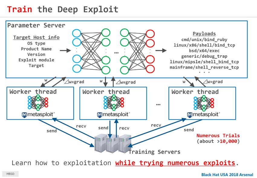
Contents
1 Introduction                                                                                               2
  1.1 Quick Guide to Neural Networks        .   .   .   .   .   .   .   .   .   .   .   .   .   .   .   .    4
  1.2 How it works . . . . . . . . . . .    .   .   .   .   .   .   .   .   .   .   .   .   .   .   .   .   17
       1.2.1 Biometric Scanners . . . .     .   .   .   .   .   .   .   .   .   .   .   .   .   .   .   .   17
       1.2.2 Intrusion Detection . . . .    .   .   .   .   .   .   .   .   .   .   .   .   .   .   .   .   19
       1.2.3 Anti-Virus . . . . . . . . .   .   .   .   .   .   .   .   .   .   .   .   .   .   .   .   .   21
       1.2.4 Translators . . . . . . . .    .   .   .   .   .   .   .   .   .   .   .   .   .   .   .   .   23
       1.2.5 Offensive Tools . . . . . .    .   .   .   .   .   .   .   .   .   .   .   .   .   .   .   .   23

2 Methods                                                                                                   25
  2.1 Attacking Weights and Biases . .      .   .   .   .   .   .   .   .   .   .   .   .   .   .   .   .   25
  2.2 Backdooring Neural Networks . .       .   .   .   .   .   .   .   .   .   .   .   .   .   .   .   .   27
  2.3 Extracting Information . . . . . .    .   .   .   .   .   .   .   .   .   .   .   .   .   .   .   .   29
  2.4 Brute-Forcing . . . . . . . . . . .   .   .   .   .   .   .   .   .   .   .   .   .   .   .   .   .   31
  2.5 Neural Overflow . . . . . . . . . .   .   .   .   .   .   .   .   .   .   .   .   .   .   .   .   .   33
  2.6 Neural Malware Injection . . . . .    .   .   .   .   .   .   .   .   .   .   .   .   .   .   .   .   35
  2.7 AV Bypass . . . . . . . . . . . . .   .   .   .   .   .   .   .   .   .   .   .   .   .   .   .   .   37
  2.8 Blue Team, Red Team, AI Team .        .   .   .   .   .   .   .   .   .   .   .   .   .   .   .   .   38
  2.9 GPU Attacks . . . . . . . . . . .     .   .   .   .   .   .   .   .   .   .   .   .   .   .   .   .   40
  2.10 Supply Chain Attacks . . . . . .     .   .   .   .   .   .   .   .   .   .   .   .   .   .   .   .   42

3 Conclusion                                                                                                44

1    Introduction
Disclaimer: This article and all the associated exercises are for
educational purposes only.
    When one looks for information on exploiting neural networks or using
neural networks in an offensive manner, most of the articles and blog posts
are focused on adversarial approaches and only give a broad overview of how
to actually get them to work. These are certainly interesting and we will
investigate what ”adversarial” means and how to perform simplified versions
of these attacks, but our main focus will be on all the other methods that
are easy to understand and exploit.
    Sadly, we can’t cover everything. The topics we do include here were cho-
sen because we feel they provide a good basis to understand more complex
methods and allow for easy to follow exercises. We begin with a quick in-
troduction to neural networks and move on to progressively harder subjects.

                                     2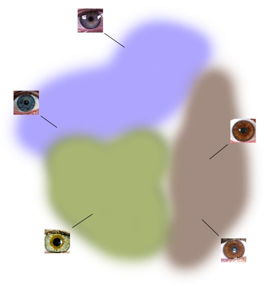
The goal is to point out security issues, demystify some of the daunting as-
pects of deep learning and show that its actually really easy to get started
and mess around with neural networks.
Who its for: This article is aimed at anyone that is interested in deep
learning from a security perspective, be it the defender faced with a sudden
influx of applications utilizing neural networks, the attacker with access to a
machine running such an application or the CTF-participant who wants to
be prepared.
How to setup: To be able to work on the exercises, we need to prepare our
environment. For speed, it is advisable to use a computer with a modern
graphics card. We will also need:

  1. Python and pip: Download and install Python3 and its package
     installer pip using a package manager or directly from the website
     https://www.python.org/downloads/.

  2. Editor: An editor is required to work with the code, preferably one
     that allows code highlighting for Python. Vim/Emacs will do. For
     reference, all exercises were prepared using Visual Studio Code https:
     //code.visualstudio.com/docs/python/python-tutorial.

  3. Keras: Installing Keras can be tricky. We refer to the official installa-
     tion guide at https://keras.io/#installation and suggest Tensor-
     Flow as a backend (using the GPU-enabled version, if one is available
     on the machine) as it is the most prevalent in industry [21].

  4. NumPy, SciPy and scikit-image: NumPy and SciPy are excel-
     lent helper packages, which are used throughout all exercises. Follow-
     ing the official SciPy instructions should also install NumPy https:
     //www.scipy.org/install.html. We will also need to install scikit-
     image for image loading and saving: https://scikit-image.org/
     docs/stable/install.html.

  5. NLTK: NLTK provides functionalities for natural language processing
     and is very helpful for some of the exercises. https://www.nltk.org/
     install.html.

  6. PyCuda: PyCuda is required for the GPU-based attack exercise. If
     no nVidia GPU is available on the machine, this can be skipped https:
     //wiki.tiker.net/PyCuda/Installation.

                                      3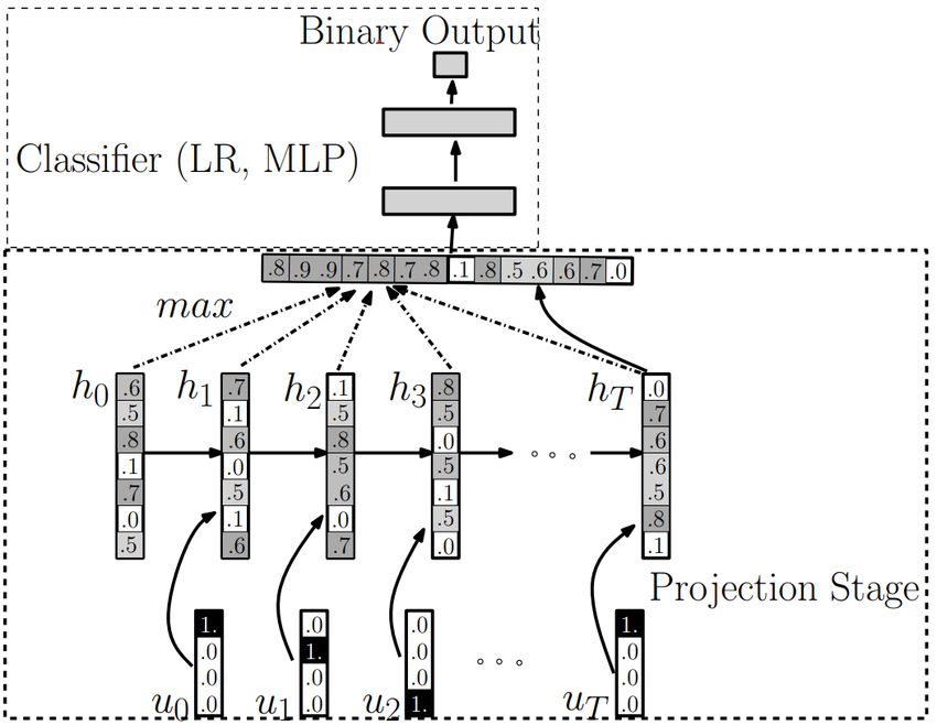
What else to know:

   • The exercises convey half of the content and it is recommended to at
     least look at them and their solutions. While it is helpful to have a
     good grasp of python, a lot of the exercises can be solved with basic
     programming knowledge and some tinkering.

   • All code is based on open-source deep learning code, which was modified
     to work as an exercise. This is somewhat due to laziness, but mainly
     because this is the actual process a lot developers follow: Find a paper
     that seems to solve the problem, test out the reference implementation
     and tweak it until it works. Where applicable, a reference is given in
     the code itself to what it is based on.

   • This is meant as a living document. Should an important reference be
     missing or some critical error still be present in the text, please contact
     the author.

1.1    Quick Guide to Neural Networks
In this section, we will take a quick dive into how and why neural networks
work, the general idea behind learning and everything we need to know to
move on to the next sections. We’ll take quite a different route compared
to most other introductions, focusing on intuition and less on rigor. If you
are familiar with the overall idea of deep learning, feel free to skip ahead.
As a better alternative to this introduction or as a supplement, we suggest
watching 3Blue1Brown’s YouTube series [53] on deep learning.
    Let’s take a look at a single neuron. We can view it as a simple function
which takes a bunch of inputs x1 , · · · , xn and generates an output f (~x).
Luckily, this function isn’t very complex:

      z(~x) = w1 x1 + · · · + wn xn + b ,                                   (1)

which is then put through something called an activation function a to get
the final output

      f (~x) = a(z(~x)) .                                                   (2)

    All the inputs xi are multiplied by the values wi , to which we refer to
as weights, and added up together with a bias b. The following activation
function a(·) basically acts as a gate-keeper. One of the most common such
activation functions is the ReLU [19][14], which has been, together with its
variants, in wide use since 2011. ReLU is just the a(·) = max(0, ·) function,

                                        4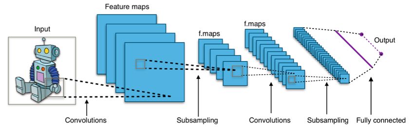
which sets all negative outputs to 0 and leaves positive values unchanged, as
can be seen in Figure 1.

                                   ReLU

                                                         x

                     Figure 1: The rectified linear unit.

   In all we can thus write our neuron simply as

     f (~x) = max(0, w1 x1 + · · · + wn xn + b) .                         (3)

    This is admittedly quite boring, so we will try to create something out of
it. Neurons can be connected in all sorts of ways. The output of one neuron
can be used as the input for another. This allows us to create all sorts of
functions by connecting these neurons. As an example, we will use the hat
function, which has a small triangular hat at some point and is 0 almost
everywhere else, as shown in Figure 2.

                                    h(x)

                                                         x

                      Figure 2: A single hat function.

   We can write down the equation for this function as follows:

                               ci − x                x − ci
    hi = max 0, 1 − max 0,               − max 0,                     .   (4)
                             ci − ci−1              ci+1 − ci
    By comparing this with Equation 3, we can see that this is equivalent to
connecting three neurons as in Figure 3 and setting the weights and biases
to the correct values by hand. We often refer to a group of neurons as a
layer, where those that connect to the input are the input (first) layer, the

                                       5
neurons that connect to the input layer are the second layer and so forth, up
until the last one that produces an output, also known as the output layer.
Every layer that is neither an input or an output layer is also referred to as
a hidden layer.
Input Output
h(x)
Figure 3: A hat function h(x) represented by 3 neurons and their connections.
In essence, this is our first neural network that takes some value x as
input and returns 1 if it is exactly ci or something less than 1 or even 0 if it
is not (we can see this by plugging in values by hand or taking a look back
at Figure 2). Essentially, we made an ci detector, as that is the only value
that returns 1. Again, not very exciting.
The beauty of hat functions, however, is that we can simply add up
multiple copies of them create a piecewise linear approximation of some other
function g(x), as shown in Figure 4. All that needs to be done is to choose
g(c1 ), · · · , g(cn ) as the height of each hat function peak.
hi (x)
f (x)
·g(ai )
x
hi+1 (x) +
x
·g(ai+1 ) ai ai+1
x
Figure 4: Piecewise approximation of some arbitrary function (blue) using
multiple hat functions (red).
This is equivalent to having the neural network shown in Figure 5, with
6all the weights and biases set to the appropriate values. Again, this is all
still done by hand, which is not what we actually want.
h1
Input f (x) Output Input Output
h2
..
.
Figure 5: Approximation of a non-linear block (left) by a network of classical
neurons with ReLU activation functions (right). The individual hat functions
are highlighted as red dashed rectangles and aggregated using an additional
neuron.
This idea can be easily extended to higher-dimensional hat functions with
multiple inputs and multiple outputs (As an example, see the case of two
outputs in Figure 6). Doing this allows us to construct a neural network that
can approximate any function. As a matter of fact, the more neurons we add
to this network, the closer we can get to the function we want to approximate.
In essence we have explored how neural networks can be universal function
approximators [8].
..
. hi
Output 1
Input
Output 2
.. h̃i
.
Figure 6: Example of a single hat function (red, dashed) being reused (blue,
dotted) to produce a different output.
But everything discussed so far is not how neural networks are designed
and constructed. In reality, neurons are connected and then trained, without
knowing the actual function g(~x) we’ve used thus far. The training process
essentially takes a bunch of data and attempts to find the best weights and
biases to approximate this data by itself, replacing our hand-designed ap-
proach. In general, these weights and biases will not resemble hat functions
7or anything similar. But, as we are still using ReLU, the final function de-
scribed by a network that was trained instead of hand-designed, will still
look like a piecewise linear interpolation. It just happens that the training
process automatically found optimal support points (similar to those of our
hat functions) based on the training data.
Let’s describe this training process in more detail. It relies on a mathe-
matical tool called backpropagation [15]. Imagine neural networks and back-
propagation as an assembly line of untrained workers that want to build
a smartphone. The last employee (layer) of this assembly line only knows
what the output should be, but not how to get there. He looks at a fin-
ished smartphone (output) and deduces that he needs some screen and some
”back” element that holds the screen. So, he turns to the employee that is
just to his left and tells him: ”You need to produce a screen and a back
element”. This employee, knowing nothing, says ”sure”, looks at these two
things and tries to break it down even further. He turns to his left to tell
the next employee, that he needs ”a piece of glass, a shiny metal and some
rubber” and that neighbor will say ”sure”. This goes on all the way through
the assembly line to the last employee, who is totally confused how he should
get his hands on ”a diamond, a car and some bronze swords”, if all he has
is copper, silicon and glass (inputs). He won’t say ”sure”, as he can’t make
what his neighbor wants. So he tells him what he can make. At this point,
the foreman will step in and tell them to start the process over, but to keep
in mind what they learned the first time around. Over time, the assembly
line employees will slowly figure a way out that works.
So how does backpropagation really work? The idea is to have a measure
of how well the current model approximates the ”true” data. This measure is
called the loss function. Assume we have a training pair of inputs ~x and the
corresponding correct outputs ~y . This can be an image (~x) and what type of
object it is (~y ). Now, when we input ~x into our neural network model, we get
some output ~ỹ, which is most likely very different to the correct value ~y , if
we haven’t trained it yet. The loss function l assigns a value to the difference
between the true ~y and the one our model calculates at this exact moment ~ỹ.
How we define this loss is up to us and will have different effects on training
later on. A simple example for a loss function is the square loss
l(~y , ~ỹ) = (~y − ~ỹ)2 . (5)
It makes sense to rewrite this in a slightly different way. Let’s use f to
denote our neural network model and θ~ = [w0 , · · · , wn , b0 , · · · , bm ] to be a
~ to mean that our
vector of all our weights and biases. We write ~ỹ = f (~x|θ)
model produces the output ~ỹ from inputs ~x based on the weights and biases
8~ In our example, this is equivalent to the foreman complaining: ”If you
θ.
continue with your work in this way (θ), ~ the smartphones you produce (~ỹ)
from this set of raw materials (~x) will look only 25% (l) like the smartphone
we are meant to produce (~y ).”
We, however, have a lot of data points (~xi , ~yi ) and want some quantity
that measures how the neural network performs on these as a whole, where
some might fit better than others. This is called the cost function C(θ), ~
which again depends on the model parameters. The most obvious would be
to simply add up all the square losses of the individual data points and take
the mean value. As a matter of fact, that is exactly what happens with the
mean squared error (MSE):
n n
~ = 1 ~ 2= 1
X X
MSE(θ) (~yi − f (~xi |θ)) ~
l(~y , f (~xi |θ)) . (6)
n i n i
As the name suggests, the cost measures the mean of all the individual
losses. In our example, this is equivalent to the foreman calculating how bad
the employees have performed over an entire batch of smartphones. Note
that it is quite typical to write the cost function name MSE instead of C.
Further, because they are so similar in nature, in a lot of articles the words
”loss” and ”cost” are used interchangeably and it becomes clear from context
which is meant.
Again, this cost function measures how far off we are with our model,
based on the current weights and biases θ~ we are using. Ideally, if we have
a cost of 0, that would mean we are as close as possible with our model to
the training data. This, however, is seldom possible. Instead, we will settle
for parameters θ~ that minimize the cost as much as possible and our goal is
to change our weights and biases in such a way, that the value of the cost
function goes down. Let’s take a look at the simplest case and pretend that
we only have a single parameter in θ. ~ In this case, we can imagine the cost
as a simple function over a single variable, say one single weight w, as shown
in Figure 7.
9C(w)
w
w̃a w̃b
Figure 7: An example cost function C for the simplest case of a single weight
parameter w. We find at least two local minima w̃a and w̃b , where w̃a might
even be a global minimum.
From the graph we see that we achieve the lowest cost if our weight has
a value of w̃a . However, in reality, we don’t see this graph. In order to draw
this graph, we had to compute the cost for every possible value of w. This
is fine for a single variable, but our neural network might have millions of
weights and biases. There isn’t enough compute power in the world to try
out every single value combination for millions of such parameters.
There is another solution to our problem. Consider Figure 8.
C(w)
w
Start
Figure 8: Instead of looking for the minimum by checking all values individ-
ually, we begin at some point (start) and move ”downhill” (red arrows) until
we reach a minimum.
Let’s pretend we started with some value of w that isn’t at the minimal
cost and we have no idea where it might be. What we do know is that the
10minimal cost is at the lowest point. If we can measure the slope at the point
we are at at the moment, then at least we know in what direction we need
to move in order to reduce our cost. And if we keep repeating this process,
i.e., measuring the slope and going ”downhill”, we should reach the lowest
point at some stage.
This should be familiar from calculus. Measuring the slope in respect to
some variable is nothing more than taking the derivative. In our case, that
is ∂C(w)
∂w
. Let’s rewrite this in terms of all parameters θ~ and introduce the
gradient
" #
∂C( ~
θ) ∂C( ~ ∂C(θ)
θ) ~ ∂C( ~
θ)
∇C(θ)~ = ,··· , , ,··· , . (7)
∂w0 ∂wn ∂b0 ∂bm
To find better parameters that reduce the cost function, we simply move
a tiny step of size α into the direction with the steepest gradient (going
downhill the fastest). The equation for which looks like this:
θ~ (new) = θ~ (old) − α · ∇C(θ~ (old) ) . (8)
This is called gradient descent, which is an optimization method. There
are hundreds of variations of this method, which may vary the step size α
(also known as the learning rate) or do other fancy things. Each of these
optimizers has a name (Adam [28], RMSProp [23], etc.) and can be found in
most deep learning libraries, but the exact details aren’t important for this
article.
Using gradient descent, however, does not guarantee we find the lowest
possible cost (also known as the global minimum). Instead, if we take a look
at Figure 9, we see that we might get stuck in some valley that isn’t the
lowest minimum, but only a local minimum. Finding the global minimum is
probably the largest unsolved challenge in machine learning and can play a
role in the upcoming exercises.
11C(w)
w
Start
Figure 9: We started at a point that leads us to a local minimum. We might
get stuck there and never even know that it is just a local minimum and not
a global one.
Next, all we need to do is to calculate ∇C(θ),~ which is done iteratively
by backpropagation. We won’t go into the exact detail of the algorithm, as
it is quite technical, but rather try to give some intuitive understanding of
what is happening. At first, finding the derivative of C seems daunting, as it
entails finding the derivative of the entire neural network. Let’s assume we
have a single input x, a single output y and a single neuron with activation
function a and weight w with no bias, i.e., the example we have been working
with so far. We want to find ∂C(w)∂w
, which seems hard. But, notice that C
contains our model f = a(w · x), which means we can apply the chain rule
in respect to a:
∂C(w) ∂C(w) ∂a
= . (9)
∂w ∂a ∂w
This is quite a bit easier to solve. As a matter of fact, if we are using the
MSE cost, we quickly find the derivative of Equation 6 to be
∂C(w)
= (y − a) . (10)
∂a
∂a
Now we just need to find ∂w . Recall that we introduced z = w~ · ~x + b as an
intermediary step in a neuron (Equation 1), which is the value just before it
is piped through an activation function a. For our case we just have z = wx.
We use the chain rule again, but this time in respect to z:
∂a ∂a ∂z
= . (11)
∂w ∂z ∂w
12We find that ∂a
∂z
is just the derivative of the ReLU activation function, which
we can look up:
(
∂a 0 for x ≤ 0
= (12)
∂z 1 for x > 0
∂z
and ∂w = x (we ignore the ”minor” detail that obviously ReLU isn’t differ-
entiable at 0...). Multiplying it all together and we have found our gradient!
Now, what happens when we add more layers to the neural network?
∂z
Well, our derivative ∂w will no longer just be x, but rather, it will be the
∂z
activation function of the lower layer, i.e., ∂w = a(lower layer) (· · · )! From there,
∂a
we basically start back at ∂w , just with the values of the lower layer. This in
essence is the reason why this algorithm is called backpropagation. We start
at the last layer and, in a sense, optimize beginning from the back. Now,
apart from going deeper, we can also add more weights to each neuron and
more neurons to each layer. This doesn’t change anything really. We only
need to keep track of more and more indices and we have our backpropagation
algorithm.
When designing a neural network and deciding upon how long and with
what parameters to run the optimizer, we need to keep in mind the concept
of under- and overfitting. Figure 10 should give some intuition what both
these terms mean.
(a) Underfitting (b) Robust (c) Overfitting
Figure 10: Piecewise approximation of some arbitrary function (blue) using
multiple hat functions (red).
If, for example, our model just doesn’t have enough neurons to approxi-
mate the function, the optimizer will try its best to come up with something
that is close enough, but just doesn’t represent the data well enough (under-
fitting). As another example, if we have a model that has more than enough
parameters available and we train it on data far too long, the optimizer will
get too good at fitting to the data, so much so, that the neural network
almost acts like a look-up table (overfitting). Ideally, we want something in
13between under- and overfitting. However, in later sections we will see, that
for our purposes, it isn’t necessarily bad to overfit.
This wraps up the very basics of neural networks we are going to cover
and we move one level higher to see what we can do with them from a network
architecture point-of-view. Roughly speaking, we can perform two different
tasks with a network, regression and classification:
• Regression allows us to uncover the relation between input variables
and do predictions and interpolations based on them. A classical ex-
ample would be predicting stock prices. Generally, the result of a re-
gression analysis is some vector of continuous values.
• Classification allows us to classify what category a set of inputs might
belong to. Here, a typical example is the classification of what object
is in an image. The result of this analysis is a vector of probabilities in
the range of 0 and 1, ideally the sum of which is exactly 1 (also referred
to as a multinomial distribution).
Thus far, our introduction of neural networks has covered how regression
works. To do classification, we need just a few more ingredients. Obviously,
we want our output to be a vector of mainly 0s and 1s. Using ReLU on the
hidden layers is fine, but problematic on the last layer, as it isn’t bounded
and doesn’t guarantee that the output vector sums to 1. For this purpose,
we have the softmax function
e zi
softmax(z0 , · · · , zj )i = Pn zj . (13)
j e
It is quite different to all other activation functions, as it depends on all
z values from all the output neurons, not just its own. But it has to, as
otherwise it can’t normalize the output vector to add up to be exactly 1.
Even with softmax in place, training this model would be problematic.
The loss function we have used thus far, MSE, is ill suited for this task, as
miss-classifications aren’t penalized enough. We need some loss that takes
into account that we are comparing a multinomial distribution. Luckily,
there exists a loss function that does exactly that, namely the cross-entropy
loss
~ = −~y · log(f (~xi |θ))
l(~y , f (~xi |θ)) ~ . (14)
The exact details why the loss is the way it is, isn’t important for our pur-
poses. We recommend Aurélien Géron’s video [17] on the subject as an easy
to understand explanation for the interested reader.
14With the basic differences between classification and regression covered,
we move on to the different types of layers found in a neural network. So far
we have covered what is called a dense layer, i.e., every neuron of one layer
is connected to (almost) every neuron of the next layer. These are perfectly
fine and in theory, we are able to do everything with just these types of
layers. However, having a deep network of nothing more than dense layers
greatly decreases the performance while training and when using it later on.
Instead, using some intuition and reasoning, a lot of new types of layers were
introduced that reduced the number of connections to a fraction. In our
motivation using hat functions, we saw that it is possible to do quite a lot
without connecting every neuron with every other neuron.
Let’s take the example of image classification. Images are comprised of
a lot of pixels. Even if we just have a small image of size 28 × 28, we are
already looking at 784 pixels. For a dense layer and just a single neuron
for each pixel, we are already looking at 614656 connections, i.e., 614656
different weights, for a single layer. But we can be a bit smarter about this.
We can make the assumption, that each pixel has to be seen in context to the
neighboring pixels, but not those far away. So, instead of connecting each of
the neurons to every pixel, we just connect the neurons to one pixel and the
8 surrounding ones. We still have 784 neurons, but reduced the amount of
weights to 784 × 8 = 7056, as each neuron is only connected to 9 pixels in
total.
In some sense, we have made 28 × 28 small 3 × 3 regions inside of the
image. That’s still a lot. We can aggregate these results and subsample by
a factor of 2, so that the following layer only needs 14 × 14 neurons. Now,
we repeat this process and connect these 14 × 14 to 3 × 3 of the neurons of
the previous layer. In essence, we are relating the small 3 × 3 regions of the
input image to other such regions (See Figure 11 for an illustration). We then
subsample some more and are left with a grid of 7 × 7 neurons (depending
on the padding we used). With so few neurons left, it is computationally not
too expensive to start adding dense layers from this point onwards.
15Figure 11: A typical convolutional neural network. Image by Aphex34
(https://en.wikipedia.org/).
What we described here are called convolutional layers [32] and the small
regions they process are their filters and the result of each filter is referred to
as a feature. In our construction we only added one neuron for each filter, but
it is perfectly fine to add more. This entire process, including subsampling
can be seen in Figure 11. What we described as subsampling is also often
referred to as pooling or down-sampling. There are different methods to
perform subsampling, such as max-pooling [66], which just takes the largest
value in some grid.
Convolutional layers are de-facto standard in image classification and
have found their use in non-image related tasks, such as text classification.
The development of new architectures using convolutional layers is too rapid
to name them all. There have, however, been a lot of milestones worth
mentioning and looking into, such as LeNet [33], AlexNet [29], GoogleNet
[61] and ResNet [22].
So far, we have looked at purely feed-forward networks, which take an
input, process it and produce an output. However, we want to mention
what happens when we have a network that takes some input, processes
it and produces an output, but then continues taking inputs for processing
and always ”remembers” what it did at the last step. This remembering is
equivalent to passing on some hidden state to the next step. A schematic
illustration of such a network is found in Figure 12. This type of network
is called a recurrent neural network (RNN). By passing on a hidden state,
this network is ideal for sequence data. As such, they are commonplace in
natural language processing (NLP), where the network begins by processing
a word or sentence and passes on the information to the next part of the
network when it looks at the following word or sentence. After all, we do not
forget the beginning of a sentence while reading it.
16Figure 12: The general structure of recurrent neural networks. Image by
François Deloche (https://en.wikipedia.org/).
One of the first and most famous type of RNN is the long-short term mem-
ory (LSTM) [25], which is the basis for a lot of newer models, such as Seq2Seq
[59] for translating/converting sequences of text into other sequences.
1.2 How it works
Before we begin to dive into some attack methods, here is a quick breakdown
of a couple of the more interesting security implementations that employ
neural networks. There are, of course, many more applications apart from
those listed in the following. Network scanners, web application firewalls and
more can all be implemented with at least some part using deep learning. The
ones we discuss here are interesting, as the methods and exercises presented
in later sections are mainly aimed at toy versions of their actual real-life
counter-part.
We won’t go deep into each application, but rather discuss one specific
implementation for each. For a review of deep learning methods found in
cyber security, we refer to the survey by Berman et al. [3]. Isao Takaesu, the
author of DeepExploit we highlight in this section, also has a more in-depth
course on the defensive aspects of machine learning [63].
1.2.1 Biometric Scanners
There are a lot of different biometric scanners. We will be looking at iris
scanners for security access (i.e., one that tells us ”access” or ”no access”)
based on deep learning. The naive approach to implementing such a scanner
would be to train a CNN on a large set of irises for ”access” and another for
”no access”.
17This type of approach would have multiple problems, some of which will
become clear through the exercises later on. From a practical standpoint
alone, this would be unfeasible, as each new person who needs his iris to
grant ”access” would require the neural network to be re-trained.
A more sensible solution is presented by Spetlik and Razumenic [57]. An
overview of the architecture is found in Figure 13.
Figure 13: Iris verification with IrisMatch-CNN. Two irises are detected and
normalized. The normalized irises are fed into the Unit-Circle (U-C) layers.
The responses from the U-C layers are concatenated and fed into the Matcher
convolutional network. A single scalar is produced – the probability of a
match. Two irises match if the probability is greater than a given threshold.
Figure and description from [57].
The description of Figure 13 should yield some familiar terms. In essence
the iris is broken down into a set of features (we can think of them like,
iris color, deformations, etc.) using their U-C layers, which are their custom
version of convolutional layers. This is done for the input iris from the current
scan and a reference iris stored in some database. The resulting features from
both these irises are then both fed through another convolutional network,
the matcher. As the name implies, this CNN is responsible for matching the
input iris to the reference based on the features and produce a single output
value: match (1) or no match (0).
The major advantage of this approach is, that it only needs to be trained
once, as the network itself doesn’t grant access, but rather checks if two
irises match. Adding new irises, thus, only requires adding it to the reference
database.
However, it still needs to be trained to be able to extract features from
an image of an iris and to perform matching. Luckily, there are available
datasets for iris images available online, such as CASIA-IrisV4 [1].
181.2.2 Intrusion Detection
Most modern approaches to intrusion detection systems are indeed based
on combinations of machine learning methods [13], such as support vector
machines [34], nearest neighbors [35] and now deep learning. We will be
focusing on the implementation by Shone et al. [56].
Intrusion detection systems need to be fast to handle large volumes of
network data, especially if they are meant for a real-time application instead
of forensics. Any deep learning implementation should therefore be compact.
However, it must still be able to handle the diversity of the data and protocols
found in a network.
Figure 14: The proposed intrusion detection architecture. Figure from [56].
The architecture proposed by Shone et al. shown in Figure 14 is compact
enough to do fast computations. The overall idea is to use a neural network to
take the 41 input features of the KDD1999/NSL-KDD dataset [52][12] found
in Table 1 and encode them into a smaller set of 28 features, which are better
suited for classification using a different machine learning method, random
forest. In other words, the neural network is used basically to pre-processes
the data.
191 duration 22 is guest login
2 protocol type 23 count
3 service 24 srv count
4 flag 25 serror rate
5 src bytes 26 srv serror rate
6 dst bytes 27 rerror rate
7 land 28 srv rerror rate
8 wrong fragment 29 same srv rate
9 urgent 30 diff srv rate
10 hot 31 srv diff host rate
11 num failed logins 32 dst host count
12 logged in 33 dst host srv count
13 num compromised 34 dst host same srv rate
14 root shell 35 dst host diff srv rate
15 su attempted 36 dst host same src port rate
16 num root 37 dst host srv diff host rate
17 num file creations 38 dst host serror rate
18 num shells 39 dst host srv serror rate
19 num access files 40 dst host rerror rate
20 num outbound cmds 41 dst host srv rerror rate
21 is host login
Table 1: Features of the network data found in the KDD1999 dataset [52].
This idea of encoding the input features into something that is easier
to work with is common in deep learning and we saw that the iris scanner
essentially did the same with its feature extractor.
Let’s focus on the datasets used for training. From the table of features
for the KDD1999/NSL-KDD dataset, it should be clear that this is a very
shallow inspection of network traffic, where the packet’s content is largely
ignored. From the architecture we know inspection happens on a per-packet
basis. This allows us draw some first conclusions: It does not take into
account the context the packet was send in (”is this well-formed but unusual
user behavior?”) and the timing (”is it a beacon?”).
Our main takeaway here is, that without deeper knowledge of what the
layers do and how random forest works, we are already able to formulate
possible attack plans, just by looking at the architecture and the training
data. In contrast, were we to find LSTM layers in the neural network’s ar-
chitecture, it would give some indication that the system might be analyzing
sequences of packets, possibly making it context-sensitive and mitigating our
20planned attack path.
Newer datasets, such as CICIDS2017 [12], use pcap files. These reflect real
world scenarios more accurately. CICIDS2017 contains the network behavior
data for 25 targets going about their daily business or facing an actual attack.
These attacks include all sorts of possible attack vectors, such as a DoS or
an SQL injection. While this dataset does not cover the entire MITRE
ATT&CK Matrix [7], it does provide enough hints at what neural network
based NIDS are possibly looking for.
1.2.3 Anti-Virus
Anti-Virus software is another prominent type of application that utilizes
machine learning. As previously, we follow a specific implementation for our
discussion. Here we use the deep learning architecture proposed in [47].
The approach they chose was to identify malicious code by what API calls
it makes and in what order. To apply deep learning to this method, the API
calls the code makes need to be preprocessed into a representation a neural
network can understand. For this, one can use a vector, where each element
in the vector represents one type of API call. We set all the elements of that
vector to 0, except for the element that represents the API call made at the
moment, which we set to 1. This is also referred to as one hot encoding.
Now, with a sequence of API calls represented as a sequence of one-
hot encoded vectors, we can feed these into an RNN for classification. The
proposed architecture by Pascanu et al. is found in Figure 15.
21Figure 15: An RNN for malware classification. Figure from [47].
What is interesting to note here, is that the dataset the proposed RNN
was trained on was not published with the paper. This is often both a security
measure (as we will see in the exercises, having access to the training set can
be very helpful for bypassing) or a matter of keeping an advantage over the
competition.
However, there are publicly available datasets, such as the Microsoft’s
malware classification challenge [51] posted on Kaggle [27] (note that the
paper that did not publish its dataset is also from Microsoft).
Kaggle itself is an interesting resource. It is a platform for corporations or
institutions to post machine learning challenges, where anyone can try their
hand at coming up with the best algorithm to perform the task and win
substantial prizes. Such challenges can be anything from predicting stock
prices based on news data to, as we saw here, classifying malware.
Every challenge must of course provide some data for the participant to
test their method on. Furthermore, the models the participants provide are
often public. This is where it becomes interesting for the security expert. On
the one hand, one can study the methods others come up with in order to
22solve a problem, on the other hand, one can look at the problem itself and
the dataset to deduce security implications. What features are available in
the dataset? Is it a sequence of data or individual data points? As we saw
earlier in our intrusion detection case, this knowledge will come in handy.
1.2.4 Translators
It might seem strange that after biometric scanners, intrusion detection sys-
tems and anti-virus we now turn to language translation. The first three
have obvious security implications, but translation?
Well, it turns out that deep learning based language translators are quite
interesting both from a defensive standpoint, as well as an offensive stand-
point. We will be looking at both these cases in the exercises. For now, let’s
assume we have a website with a chatbot running, but the developer was too
lazy to localize it into all languages. Instead, the developer simply wrote the
chatbot in english and slapped a translator neural network on top.
The almost classical translator to use is the Sequence to Sequence (Seq2Seq)
model [59]. Seq2Seq is based on LSTM and maps a sequence of characters
to another sequence of characters, depending on what it was trained on. An
english sentence can be mapped to a german sentence using this model, a
schematic view of which is shown in Figure 16.
Figure 16: The model reads an input sequence ”ABC” and produces
”WXYZ” as the output sequence. The model stops making predictions after
outputting the end-of-sentence token. Figure and description from [59].
Translators are interesting, because they might not seem security relevant
to the person implementing it on a website or similar. In our discussion, it
shall serve as an example of a non-security related deep learning tool which
we exploit in a later exercise.
1.2.5 Offensive Tools
The final area we want to highlight that has started to incorporate deep
learning is automated penetration testing. Specifically, we will take a short
23look at DeepExploit created by Isao Takaesu at Mitsui Bussan Secure Direc-
tions [62]. While it won’t make an appearance in the exercises, we include it
as it is probably the most interesting use of deep learning in offensive security
so far.
DeepExploit performs the typical chain of intelligence gathering, exploita-
tion, post-exploitation, lateral movement and report generation fully auto-
matic. It does this by generating commands for Metasploit [50], which per-
forms the actual execution.
While not all steps in the chain utilize machine learning, the information
gathering and main exploitation phase do. For example, DeepExploit is able
to analyze HTTP responses using machine learning to predict what kind of
stack is deployed on the target.
But the truly interesting part comes from the exploitation phase. In
Figure 17 an overview of the training process is shown. DeepExploit uses re-
inforcement learning [60] to improve its exploitation capability and is trained
asynchronously [42] on multiple training servers. In reinforcement learning
one doesn’t have a training set, but rather one lets an agent explore a huge
amount of possible actions. A reward function tells the agent if the chosen
actions were successful or not and it learns from these and is able to repeat
and modify them in the future, should a similar situation arise.
24Figure 17: An overview of the training process for DeepExploit. Figure from
Isao Takaesu’s presentation at Black Hat USA 2018 Arsenal [62].
2 Methods
In the following we introduce some of the methods that can be used to
exploit neural networks or incorporated into an offensive tool. We tried to
structure the order of these methods by category and increasing difficulty of
the exercises. Holt gives a nice and accessible survey of related methods in
[26].
2.1 Attacking Weights and Biases
Let’s assume we have gained partial access to an iris scanner which we want
to bypass. While we can’t access any of the code, we have full access to the
’model.h5’ file, which holds all the information for a neural network.
The first thing to note is that the ’model.h5’ file is using a Hierarchical
Data Format (HDF5) [18], which is a common format to store the the model
information and also data. There are other formats to store this in, such
as pure JSON, but for illustrative purposes we will stick to HDF5. Further,
25as this file format is used in many different applications apart from deep
learning, tools to view and edit are easy to find.
As HDF5 files can become quite large, it is not uncommon to have a
separate source control for these files or store them in a different location
compared to the source code in production. This can lead to the scenario
presented here, where someone forgot to employ the same security measures
to both environments.
Having access to the model file is almost as good as having access to code
or a configuration file. Keras [6], for example, uses the model file to store
the entire neural network architecture, including all the weights and biases.
Thus, we are able to modify the behavior of the network by doing careful
edits.
A biometric scanner employing neural networks will most likely be doing
classification. This can be a simple differentiation between ”Access Granted”
and ”Access Denied”, or a more complex identification of the individual being
scanned, such as ”Henry B.”, ”Monica K.” and ”Unknown”. Obviously we
want to trick the model into misclassifying whatever fake identification we
throw at it by changing the HDF5 file.
There are of course restrictions to what we can modify in this file without
breaking anything. It should be obvious that changing the amounts of inputs
or outputs a model has will most likely break the code that uses the neural
network. Adding or removing layers can also lead to some strange effects,
such as errors occurring when the code tries to modify certain hyperparam-
eters.
We are, however, always free to change the weights and biases. It won’t
make much sense to try and fiddle around with just any values, because at
the time of writing, the field of deep learning still lacks a good understanding
and interpretation of the individual weights and biases in most layers. For
the last layer in a network, however, things get a bit easier. Take a look at
the network snapshot in Figure 18.
w
~ = (0.2, 0.5, 1.2) b = 0.7
w −0.1
~ = (−0.5, 0.4, −0.3) b = 100000.0
Figure 18: A neural network with one of the output’s bias set to a very
high value, which completely overshadows the contribution from the weights
multiplied by the input.
26Here we spiked the bias for one of the final neurons in a classification
network. By using such a high value, we almost guarantee that the classifier
will always mislabel every input with that class. If that class is our ”Access
Granted”, any input we show it, including some crudely crafted fake iris,
will get us in. Alternatively, we can also set all weights and biases of the
last layer to 0.0 and only keep the bias of our target neuron at 1.0. Which
method to choose depends on how stealthy it should be.
Generally, this sort of attack works on every neural network doing clas-
sification, if we have full access to the model. It is also possible to perform
this type of attack on a hardware level [4]. For a more advanced version of
directly attacking the weights and biases in a network, we also refer to the
work by Dumford and Scheirer [10].
Blue-Team: Treat the model file like you would a database storing sensi-
tive data, such as passwords. No unnecessary read or write access, perhaps
encrypting it. Even if the model isn’t for a security related application, the
contents could still represent the intellectual property of the organization.
Exercise 0-0: Analyze the provided ’model.h5’ file and answer a set of
multiple choice questions.
→ https://github.com/Kayzaks/HackingNeuralNetworks/tree/master/
0_LastLayerAttack
Exercise 0-1: Modify a ’model.h5’ file and force the neural network to
produce a specific output.
→ https://github.com/Kayzaks/HackingNeuralNetworks/tree/master/
0_LastLayerAttack
2.2 Backdooring Neural Networks
We continue with the scenario from the previous section. However, our goal
now is to be far more subtle. Modifying a classifier to always return the
same label is a very loud approach to breaking security measures. Instead,
we want the biometric scanner to classify everything as usual, except for a
single image: Our backdoor.
Being subtle is often necessary, as such security systems will have checks
in place to avoid someone simply modifying the network. But, these security
checks can never be thorough and cover the entire input spectrum for the
network. Generally, it will simply check the results for some test set and
verify that these are still correctly classified. If our backdoor is sufficiently
27different from this unknown test set (an orange iris for example), we should
be fine.
Note that when choosing a backdoor, it is advisable to not choose some-
thing completely different. Using an image of a cat as a backdoor for an iris
scanner can cause problems, as most modern systems begin by performing
a sanity check on the input, making sure that it is indeed an iris. This is
usually separate from the actual classifier we are trying to evade. But, of
course, if we have access to this system as well, anything goes.
At first glance it would seem that we need to train the model again from
scratch and incorporate the backdoor into the training set. This will work,
but having access to the entire training set the target was trained on is often
not the case. Instead, we can simply continue training the model as it is in
its current form, using the backdoor we have.
There really isn’t much more to poisoning a neural network. Generally
all the important information, such as what loss function was used or what
optimizer, is stored in the model file itself. We just have to be careful of
some of the side effects this can have. Continuing training with a completely
different training set may cause catastrophic forgetting [40], especially con-
sidering our blunt approach. This basically means, that the network may
loose the ability to correctly classify images it was able to earlier. When this
happens, security checks against the network might fail, signaling that the
system has been tempered with.
If the model does not contain the loss function, optimizer or any other
parameters used for training, things can get a bit trickier. If we are faced
with such a situation, our best bet is to be as minimally invasive as possible
(very small learning rate, conservative loss function and optimizer) and stop
as soon as we are satisfied the backdoor works. This must be done, as modern
deep learning revolves a lot around crafting the perfect loss function and it
is entirely possible that this information is inaccessible to us. We will, thus,
slide into some unintended minima very quickly, amplifying the side effects
mentioned earlier.
Exercise 1-0: Modify a neural network for image classification and force it
to classify a backdoor image with a label of choice, without miss-classifying
the test set.
→ https://github.com/Kayzaks/HackingNeuralNetworks/tree/master/
1_Backdooring
Now, apart from further training a model, if we have access to some
developer machine with the actual training data, we can of course simply
inject our backdoor there and let the developer train the model for us.
28In [5], Chen et al. introduce the idea of data poisoning and backdooring
neural networks. We also refer to [38] for another, more advanced version of
this attack. Furthermore, for PyTorch,
Blue-Team: There are methods designed to mitigate the effects of back-
dooring and poisoning, such as fine-pruning [37] and AUROR [55]. However,
most methods are aimed at the initial training process and not at models
in production. One quick to implement measure is to perform sanity checks
against the neural network using negative examples periodically. Make sure
that false inputs return a negative result and try to avoid testing positive
inputs or else you might have another source of possible compromise.
2.3 Extracting Information
Neural networks, in some sense, have a ”memory” of what they have been
trained on. If we think back to our introduction and Figure 10, the network
stores a graph that sits on or somewhere in between the data points. If we
only have that graph, it seems possible to make guesses at to where these
data points might have been in the first place. Again, take Figure 10 and
think away the data points. We would be quite close to the truth by assuming
that choosing random points slightly above or below the graph would yield
actual data points the network was trained on.
In other words, we should be able to extract information from the neural
network that has some resemblance to the data it was trained on. Under
certain circumstances, this turns out to be true, such Hayes et al. [20] and
Hitaj et al. [24] have shown, with both groups leveraging Generative Adver-
sarial Networks (GANs). This is actually quite a big privacy and security
problem. Being able to extract images a neural network was trained on can
be a nightmare.
However, this is only true to some extent. As neural networks are able to
generalize and are mostly trained on sparse data, the process of extracting
the original training set is quite fuzzy and generates a lot of false-positives.
I.e., we will end up with a lot of examples that certainly would pass through
the neural network as intended, but not resemble the original training data
in the slightest.
While the process of extracting information that closely resembles the
original data is interesting in itself, for us it is perfectly sufficient to generate
these incorrect samples. We don’t need the exact image of the CEO to bypass
facial recognition, we only require an image that the neural network thinks
is the CEO. Luckily, these are quite easy to generate.
29We can actually train a network to do exactly this, by misusing the power
of backpropagation. Recall that backpropagation begins at the back of the
network and subsequently ”tells” each layer how to modify itself to generate
the output the next one requires. Now, if we take an existing network and
simply add some layers in-front of it, we can use backpropagation to tell these
layers how to generate the inputs it needs to produce a specific output. We
just need to make sure to not change the original network and only let the
new layers train, as shown in Figure 19.
Figure 19: We connect a single layer of new neurons (blue, dashed) in front
of an existing network (red, dashed). We only train the new neurons and
keep the old network unchanged.
For illustration, recall the assembly line example from our introduction.
We have a trained assembly line that creates smartphones from raw materials.
As an attacker, we want to know exactly how much of each material this
company uses to create a single smartphone. Our approach above is similar
to sneakily adding an employee to the front of the assembly and let him ask
his neighbor what and how much material he should pass to him (learning
through backpropagation).
Exercise 2-0: Given an image classifier, extract an image sample that will
create a specific output.
→ https://github.com/Kayzaks/HackingNeuralNetworks/tree/master/
2_ExtractingInformation
Blue-Team: Think about cryptographic methods [9][43], such as encrypting
your model/data and secure computing. See also Jason Mancuso’s talk at
DEFCON 27 AI Village [39].
302.4 Brute-Forcing
Brute-forcing should be reserved for when all other methods have failed.
However, when it comes to breaking neural networks, a lot of approaches
somewhat resemble brute-forcing. After all, training itself is simply showing
the network a very large set of examples and have it learn in a ”brute-force”
type of manner. But here we are truly talking about brute-forcing a target
network over a wire in the classical sense, instead of training it locally.
Just as brute-forcing a password, we can use something similar to a dic-
tionary attack. A dictionary attack assumes that the user used normal words
and patterns as part of the password and we can do the same for neural net-
works. The idea is to start with some input that seems reasonable and could
possibly grant access and slightly modifying it until we get in.
Let’s take the iris scanner as an example again. If we know the CEO’s
iris works and know that he or she has blue eyes, but don’t have an actual
picture, we begin with any image of a blue iris of some random person and
start modifying it until we get in. This might seem difficult, how does one
modify an iris to match and what features are important? But, it turns out
it suffices to simply add some mild, unspecific randomness to the image. In
essence, we are probing around images of a blue iris and hope that something
nearby will be ”good enough”. In Figure 20 this process is highlighted.
31Figure 20: A simplified 2-dimensional representation of the possible iris im-
ages with some examples (blue, green and brown). The white area represents
all images that aren’t irises. Images that are similar to an iris (a ball) would
be in the white, but closer to the colored areas than those that aren’t (a cat).
The red circle highlights the area of images that would grant access (i.e., the
CEO’s iris and those that are very similar). The blue dot is our random
blue iris starting point and the arrows highlight how we explore nearby irises
using pure randomness, with one even hitting the target area.
In Figure 20 we have an example where it makes sense to start with a
blue iris, as it is the closest. Generally we can begin anywhere, it will just
take more exploration and at some point become infeasible. However, there
are situations where it makes sense to start with another color or even a
picture of something that isn’t an iris, such as a ball. It is interesting to
note, an image that started out as a ball and is randomly perturbed until it
gets accepted will still look like a ball, even though it passes as the CEO’s
iris, as we aren’t changing that much about the picture and just a few pixel
here and there.
An image that isn’t even remotely related to the one we are trying to
brute-force and perturbing it until the neural network mistakes it for the real
one, is called an adversarial example [16][30][46]. It is an active research topic
[67][31], especially in the field of facial recognition where one tries to bypass
or trick it using real-world props [54][68]. It should, however, be obvious that
the field isn’t trying to find ways for brute-forcing, but rather the opposite:
to avoid misclassification. Misclassification can be a huge problem for safety
critical applications, such as self-driving cars.
32Blue-Team: As with password checks, try to employ the same security
measures for any access control based on neural networks. Limit the amount
of times a user may perform queries against the model, avoid giving hints to
what might have gone wrong, etc.
Exercise 3-0: Brute-force a neural network with an adversarial approach.
→ https://github.com/Kayzaks/HackingNeuralNetworks/tree/master/
3_BruteForcing
We turn back to the approach of Section ”Extracting Information”. As
we have it now, images generated using that method will not pass standard
sanity checks that happen before a neural network (”Is there even an iris
in this picture?”), as they will mostly look like pure noise. Let’s see how
we can improve this by using an adversarial approach. So far, we have tried
creating an adversarial example against a black-box using brute-force. In a
white-box scenario, we can do far better than brute-forcing. As a matter of
fact, we can consistently create adversarial images which will perform more
reliably against sanity checks. This is by no means a trivial task and requires
in-depth knowledge. Luckily, libraries and tools exist that can perform this
for us. One such library is SecML [48], which can reduce the process of a
white-box/unrestricted adversarial attack (and others) down to a few lines
of code (see https://secml.gitlab.io/index.html for an example based
on PyTorch).
2.5 Neural Overflow
The next method we will cover is not recommended, but included as one
of the first things a security expert would think of: ”Can you overflow the
input to a neural network?”. We include it here to illustrate some interesting
properties of neural networks, that might help in exploitation. Note, an
actual feasible buffer overflow method is presented in a later section.
Let’s take a simple neural network that does classification with one input
x and one output y (so that we can visualize it better). In Figure 21, the
graph of this input-output relationship is shown.
33You can also read