Statistical Neuroscience in the Single Trial Limit
←
→
Page content transcription
If your browser does not render page correctly, please read the page content below
Statistical Neuroscience in the Single Trial Limit
                                                                              Alex H. Williams and Scott W. Linderman

                                                                                              March 10, 2021
arXiv:2103.05075v1 [q-bio.NC] 8 Mar 2021

                                                                                                   Abstract

                                                 Individual neurons often produce highly variable responses over nominally identical trials, reflecting a
                                                 mixture of intrinsic “noise” and systematic changes in the animal’s cognitive and behavioral state. In addition
                                                 to investigating how noise and state changes impact neural computation, statistical models of trial-to-trial
                                                 variability are becoming increasingly important as experimentalists aspire to study naturalistic animal
                                                 behaviors, which never repeat themselves exactly and may rarely do so even approximately. Estimating the
                                                 basic features of neural response distributions may seem impossible in this trial-limited regime. Fortunately,
                                                 by identifying and leveraging simplifying structure in neural data—e.g. shared gain modulations across
                                                 neural subpopulations, temporal smoothness in neural firing rates, and correlations in responses across
                                                 behavioral conditions—statistical estimation often remains tractable in practice. We review recent advances
                                                 in statistical neuroscience that illustrate this trend and have enabled novel insights into the trial-by-trial
                                                 operation of neural circuits.

                                           Introduction

                                           Widely disseminated optical and electrophysiological recording technologies now enable many research labs to
                                           simultaneously record from hundreds, if not thousands, of neurons. Often, a first step towards characterizing
                                           the resulting datasets is to estimate the average response of all neurons across a small set of conditions. For
                                           example, a subject may be presented different sensory stimuli (images, odors, sounds, etc.) or trained to
                                           perform different behaviors (reaching to a target, pressing a lever, etc.), each of which constitutes a different
                                           condition. Each condition is then repeated many times, and the neural response is averaged over these
                                           nominally identical trials to reduce noise and variability.

                                           Despite their obvious importance, averages represent incomplete (and potentially misleading [28]) summaries
                                           of neural data. Trial-to-trial variations in neural activity reflect a variety of interesting processes, including fluc-
                                           tuations in attention and task engagement [12• , 68• , 73, 84], changes-of-mind during decision-making [13, 23,
                                           33, 34, 69], modulations of behavioral variability to promote learning [14], representations of uncertainty [49],
                                           changes-in-strategy [72], and modified sensory processing linked to active sensing [22, 91], locomotion [94],
                                           and other motor movements [53, 88]. Some of these effects may be disentangled by developing targeted
                                           experimental designs [84] or by analyzing behavioral covariates [53, 55, 88]. In other cases, these effects
                                           may spontaneously emerge and subside during the course of an experiment and leave little to no behavioral

                                                                                                       1
signature.

While the activity of individual neurons may correlate with these single-trial phenomena, such effects may
be subtle and difficult to detect. A unique advantage to collecting simultaneous population recordings is
the possibility of pooling statistical power across many individually noisy neurons to characterize short-term
fluctuations and long-term drifts in neural circuit activity. One way to approach this goal is to estimate higher-
order statistics of the neural response distribution, such as the trial-to-trial response correlations between
all pairs of neurons. Unfortunately, as we discuss below, estimating second-order response properties (i.e.,
covariance structure) generally requires the number of trials per condition to grow super-linearly with the
number of neurons, which can quickly become infeasible. However, we will see that there are good reasons
to believe this worst-case analysis is overly pessimistic, and that it can be overcome by carefully designed
statistical analyses.

At the same time, there is a trend toward studying neural circuits in more ethologically relevant settings. This
involves studying rich sensory stimuli and spontaneous, unconstrained behaviors which elicit more natural
patterns of neural activity. Recent work in visual neuroscience, for instance, has measured activity in response
to very diverse sets of natural images [7, 95], with as little as two trials per image [87]. This starkly contrasts
with classical experiments, which presented simple stimuli (e.g. oriented gratings) repeatedly over many trials.
Similar trends are present in motor neuroscience, where motion capture algorithms have been leveraged to
measure spontaneous animal behaviors [46, 47]. Unconstrained motor actions repeat themselves infrequently
and inexactly, resulting in few “trials” compared with classical behavioral tasks (e.g. cued point-to-point reaches
or lever presses).

Figure 1A summarizes these trends. We selected a small subset of papers from the past thirty years that obtained
multi-neuronal recordings, and plotted the total number of trials collected against the number of free variables
one could potentially try to estimate. There are a total of N C such variables for a recording of N neurons across
C conditions. (For now, we neglect the within-trial temporal dynamics of neural responses; including these
dynamics as estimatable parameters would only exacerbate the potential for statistical error.) The greyscale
background shows the expected estimation error for second-order statistics under a worst-case scenario where
trial-to-trial variations are decorrelated across neurons and conditions (i.e., variability that is high-dimensional,
in a sense that we formally define below). We observe that the number of trials has been growing more slowly
than number of parameters we wish to estimate, raising the possibility that our statistical analysis will suffer
from greater estimation errors. If these trends continue, traditional experimental designs that assume large
numbers of trials over a discrete set conditions, will become an increasingly ill-suited framework for neural
data analysis—under completely unconstrained and naturalistic settings, no two experiences and actions are
truly identical so, in some sense, each constitutes a unique condition with exactly one trial.

The solution to this apparent problem is to recognize that neural and behavioral data may not be as high
dimensional as they appear. Though we may never see the exact same pattern of neural activity or postural
dynamics twice, our measurements may lie close to a low dimensional manifold. For example, the neuron-by-
neuron covariance matrix might be approximately low rank, trial-to-trial variability may arise from a small

                                                         2
A Worst-Case
Estimation Error
Zohary et al. (1994)
Hatsopoulos et al. (1998)
Chapin et al. (1999)
B condition
averages
uncorrelated
variability
correlated
variability
low high Taylor et al. (2002)
105 Hegde & Van Essen (2004)
Briggman et al. (2005)
Ohki et al. (2005)
104
PC 2
Bathellier et al. (2008)
Kaufman et al. (2013)
Allen Brain Observatory, PC 1
trials
103 natural images (2017)
Russo et al. (2018)
102 Stringer et al. (2019)
Steinmetz et al. (2019)
Musall et al. (2019)
101 0 Markowitz et al. (2019)
10 102 104 106 108 Rumyantsev et al. (2020)
neurons * conditions
Pashkovski et al. (2020)
Figure 1: (A) The number of trials in neural datasets is growing
1 more slowly the number of simultaneously recorded
neurons and sampled behavioral conditions. Scatter plot color corresponds to year of publication on an ordinal scale
(see legend). Grayscale heatmap shows the worst-case error scaling for covariance estimation [92• ]—the contours
are O(N C log N C) for a dataset with N neurons and C conditions. Darker shades correspond to larger error. (B) Low-
dimensional visualizations of trial-to-trial variability in static (top row) and dynamic (bottom row) neural responses.
Left, trial average in two conditions (blue and red). In the dynamic setting, neural firing rates evolve along a 1D curve
parameterized by time. In the static setting, responses are isolated points in firing rate space. Middle, same responses but
with independent single-trial variability illustrated in each dimension. Right, same responses with correlated variability.
The positive correlations in the top panel are “information limiting” because they increase the overlap between the
two response distributions, degrading the discriminability of the two conditions (see, e.g., [2]). In the bottom panel,
correlations in neural response amplitudes result in trajectories that are preferentially stretched or compressed along
particular dimensions from trial-to-trial (see [102• ] for a class of models that are adapted to this simplifying structure).
number of internal state variables, and natural behavior may be composed of a small number of relatively
stereotyped movements. If and when such simplifying structure is found, it can dramatically reduce the number
of trials necessary to obtain accurate parameter estimates. The success of single trial analysis of neural and
behavioral data relies crucially on our ability to identify and leverage these patterns in our data. The rest of
this review summarizes recent examples from the neuroscience literature that exemplify this approach.
Statistical challenges in trial-limited regimes
In a pioneering study from the early 1990’s, Zohary et al. [109] measured responses from co-recorded neuron
pairs over 100 sessions in primates performing a visual discrimination task. They found weak, but detectable,
correlations in the neural responses over trials—when one neuron responded with a large number of spikes,
the co-recorded neuron often had a slightly higher probability of emitting a large spike count. Though this
result may appear innocuous, the authors were quick to point out that even weak correlations could drastically
impact the signalling capacity of sensory cortex (fig. 1B). This finding inspired a large number of experimental
and theoretical investigations into “noise correlations,” which today represents one of the most developed
bodies of scientific work on trial-to-trial variability (for reviews, see [2, 36]).
The fact that Zohary et al. [109] were technologically limited to recording two neurons at once came with a
silver lining. For every variable of interest (i.e. a correlation coefficient between a unique pair of neurons),
3Box 1 — Notation
We aimed to keep mathematical notation light, but we summarize a few points of standard notation here.
We denote scalar variables with non-boldface letters (e.g. x or X ), vectors with lowercase, boldface
letters (e.g. x ), and matrices with uppercase, boldface letters (e.g., X ). The set of real numbers is
denoted by R, so the expression s ∈ R means that s is a scalar variable. Likewise, v ∈ Rn means that
v is a length-n vector, and M ∈ Rm×n means that M is a m × n matrix. A matrix X ∈ Rm×n is said
to be “low-rank” if there exist matrices U ∈ Rm×r and V ∈ Rn×r , where r < min(m, n) and for which
X = U V > . The smallest value of r for which this is possible is called the rank of X , in which case we
would say “X is a rank-r matrix.” We briefly utilize “Big O notation” to represent a function up to a
positive scaling constant. More precisely, we will use O(g(N )) to represent an anonymous function that
is upper bounded by g(N ), up to an absolute constant. That is, O(g(N )) represents any function f that
satisfies f (N ) ≤ C · g(N ) for some constant C > 0. When g is a monotonically increasing function of N ,
dropping constant terms like this is useful to understand the scaling behavior of the system in the limit
as N becomes very large.
they collected a large number of independent trials. Their statistical analyses were straightforward because
the number of unknown variables was much smaller than the number of observations. Two recent studies by
Bartolo et al. [3] and Rumyantsev et al. [74• ] revisited this question using modern experimental techniques.
The latter group recorded calcium-gated fluorescence traces from N ≈ 1000 neurons in mouse visual cortex
over K ≈ 600 trials. Since each session contained roughly N (N − 1)/2 = 499500 pairs of neurons, the number
of free parameters (correlation coefficients between unique neuron pairs) was vastly larger than the number
of independent observations. Intuitively, if the correlations between neuron pair A-B and neuron pair B-C
were mis-estimated, then the estimated correlation between neurons A and C would also likely be inaccurate,
since the same set of trials were used for the underlying calculation. The authors were forced to grapple
with an increasingly common question: how many neurons and trials must be collected to ensure the overall
conclusions were accurate?
The field of high-dimensional statistics provides answers to questions like this [92• , 97]. A standard result states
that, in order to accurately estimate a N × N covariance matrix, Σ, the number of trials should be O(d log N )
where d measures the effective dimensionality of the covariance matrix. If the tails of the neural response
distribution decay sufficiently fast, this bound can be improved to O(d) trials [93]. Formally, the dimensionality
is defined as d = Tr[Σ]/kΣk (see section 5.6 of [92• ]). Intuitively, d is large when trial-to-trial variability equally
explores every dimension of neural firing rate space (as in fig. 1B, “uncorrelated variability”). Conversely, d is
small when there are large correlations in a small number of dimensions, such that many dimensions are hardly
explored relative to high-variance dimensions. In the worst case scenario where variability is high-dimensional
and heavy-tailed, we would have d = N and require O(N log N ) trials, which may be infeasible to collect.
Fortunately, Rumyantsev et al. [74• ] provide empirical evidence and a simple circuit model which suggest
that the eigenvalues of Σ decay rapidly. This corresponds to the statistically tractable setting where d is much
smaller than N . Bartolo et al. [3] contemporaneously reported similar results under different experimental
conditions and in nonhuman primates. Overall, these works provide some of the strongest evidence to date
4that noise correlations do indeed limit the information content of large neural populations. The effect of noise
correlations more generally—e.g., in concert with behavioral state changes [54], and in response to more
diverse stimuli [71]—remains a subject of active research.
For us, the key takeaway is that the presence of simplifying structures (e.g. low dimensionality) enables
accurate statistical analysis when we collect data from many more neurons and behavioral conditions than
trials. We can leverage formal results from high-dimensional statistics to sharpen this conceptual lesson into
quantitative guidance for experimental designs.
Gain modulation and low-rank matrix decomposition
It is useful to view covariance estimation (discussed above), as a special case of maximum likelihood estimation
(MLE). Given a recording of N neurons, we observe neural responses {x 1 , x 2 , . . . , x K }, where each x k ∈ RN
is a vector holding the population response on trial k ∈ {1, 2, . . . , K}. Now, assume that each response is
sampled independently from a multivariate normal distribution with mean µ and covariance Σ; that is,
x k ∼ N (µ, Σ) for every trial index k. It is a simple exercise to show that, under a log-likelihood objective
PK
function, the maximum likelihood parameter estimates are the empirical mean, µ b = K1 k=1 x k , and the
b = 1 K (x k − µ
empirical covariance, Σ b )> .
b )(x k − µ
P
K k=1
In the last section, we discussed a scenario where the covariance was well-fit by a low-rank decomposition—i.e.,
there is some N × d matrix U, for which Σ ≈ UU > —and saw that such structure allows us to estimate the
covariance matrix accurately in a reasonable number of trials. Other modeling assumptions can achieve similar
effects. For example, Wu et al. [105• ] developed a model with Kronecker product structure to model variability
across multiple data modalities (odor conditions and neurons). Integrating data from multiple modalities into
a unified model is a nascent theme of recent research in neuroscience [20, 51, 59, 80, 102• ], and is already
well-established in other areas of computational biology [108• ].
Using a multivariate normal distribution to model single-trial responses is often mathematically convenient and
computationally expedient. However, it is usually not an ideal model. For example, if we count the number of
spikes in small time windows as a measure of neural activity, a Poisson distribution is typically used to model
variability at the level of single neurons [61]. Extending the Poisson distribution to the multivariate setting
turns out to be a somewhat advanced and nuanced subject [31]. A simple approach is to introduce per-trial
latent variables, which induce correlated fluctuations across neurons. For example, suppose the number of
spikes fired by neuron n on trial k is modeled as X nk ∼ Poisson(u >
n v k ), where u n ∈ R and v k ∈ R are vectors
r r
holding r “components” or latent variables for each neuron and trial. It is useful to reformulate this model
using matrix notation. Let Λ = U V > , where the matrices U ∈ RN ×r and V ∈ RK×r are constructed by stacking
the vectors u n and v k , row-wise. We can interpret Λ as a matrix of estimated firing rates, which, in expectation,
equals the observed spikes counts—i.e., our model is that E[X ] = Λ = U V > , where X is an N × K matrix
holding the observed spike counts, and noise is Poisson-distributed (i.i.d. across neurons and trials).
This model is a special case of a low-rank matrix factorization (Box 2)—a versatile framework that encompasses
5A firing B v C synaptic
weights
trial k
data
rate input
neuron 1 time u 1
2
amplitudes
(trial k)
3
neuron 2
neurons
4
5
6
neuron 3 7
8
trial 1 trial 2 trial 3
1 2 3 4 5 6 7 8 9
9
U vk xk
trials
D rank-3 nonnegative data
1
2
3
4
neurons
5
6
7
= + +
8
9
1 2 3 4 5 6 7 8 9
component 1 component 2 component 3
trials
E Spike-Triggered Covariance (PCA components) F firing rates over time Principal Components (PCs)
Equivalent PCs (rotated)
neurons
Spike-Triggered NMF factors
Unique NMF factors
time
Figure 2: Matrix factorization methods for single-trial analysis. (A) Schematic firing rate traces of three neurons
demonstrating correlated gain-modulation: the peak responses in all three neurons are scaled by a common factor on
each trial. (B) A rank-1 NMF model over 9 neurons and 9 trials. The neural responses on each trial are taken to be the
peak evoked firing rate as illustrated in panel A. The data X (black-to-white heatmap) are approximated by the outer
product of two vectors, u v > (respectively shown as blue and red stem plots). (C) Interpretation of a rank-3 NMF model
as an idealized neural circuit. Low-dimensional neuron factors, U, correspond to synaptic weights, while trial factors, v k
for trial k, correspond to input amplitudes (a related circuit interpretation is provided in [102• ]). (D) A schematic data
matrix containing responses from 9 neurons over 9 trials is modeled as the sum of three rank-1 components (overall, a
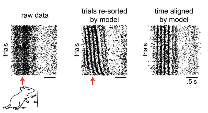
rank-3 model). (E) Spike-triggered ensemble analysis of retinal ganglion neurons in Salamander retina. NMF-identified
components correspond to localized visual inputs that correspond to presynaptic bipolar cells; these signals are mixed
together in PCA-identified components (panel adapted from [44]). (F) Demonstration of the “rotation problem” in
PCA. Left, a rank-three data matrix holding a multivariate time series. Right, temporal factors identified by PCA and
NMF (colored lines). Dashed black line denotes zero loading. In this case, the decomposition by NMF is unique (up to
permutations; [17]), unlike PCA.
6many familiar methods including PCA, k-means clustering, and others [90• ]. Now we ask: given X , what
are good values for U and V? One way to answer this question is to optimize U and V with respect to the
log-likelihood of the data. After removing an additive constant from the log-likelihood function, we arrive at
the following optimization problem:
N X
X K
maximize X nk log Λnk − Λnk
n=1 k=1 (1)
subject to Λ = U V > ; U ≥ 0; V ≥ 0.
We have included nonnegativity constraints which ensure that Λ ≥ 0; i.e., the predicted firing rates are,
quite sensibly, nonnegative. Alternatively, we could have dropped the nonnegativity constraints, and set
Λ = exp(U V > ), where the exponential is applied elementwise. However, the factor matrices are typically
easier to interpret when they are nonnegative, as demonstrated by Lee and Seung [38], who popularized the
model in eq. (1) under the name of nonnegative matrix factorization (NMF). An alternative form of NMF is
nearly identical, but uses a least-squares criterion instead of the Poisson log-likelihood (see [25] for a modern
review).
NMF is of immense importance to modern neural data analysis. Variants of this method underlie popular
algorithms for spike sorting [85], extracting calcium fluorescence traces from video [66, 107], identifying
sequential firing patterns in neural time series [45, 65], parcellating widefield imaging videos into functional
regions [78], and theories of grid cell pattern formation [18, 83]. In the context of single-trial analysis, NMF
can be interpreted as a model of gain modulation (fig. 2A), which is a widely studied phenomenon in sensory
and motor circuits [21, 63]. For example, in a rank-1 NMF model, the firing rate matrix is factorized by a pair
of vectors, Λ = u v T (fig. 2B). We can interpret u as being proportional to the trial-averaged firing rate of all N
neurons. On trial k, the predicted firing rates are Λ(:, k) = vk u, which is simply the average response re-scaled
by a per-trial gain factor, vk . It has been hypothesized that such gain modulations play a key role in tuning the
signal-to-noise ratio of sensory representations, with larger gain factors corresponding to attended inputs [68• ,
70].
NMF can also model more complex patterns of single-trial variability. In particular, an NMF model with r
low-dimensional components (i.e. a rank-r model) can capture independent gain modulations over r neural
sub-populations (fig. 2C-D). Despite differing in some important details, recent statistical models of sensory
cortex bear some similarity to this framework [68• , 98, 99]. We thus view this conceptual connection between
NMF—a general-purpose method with many applications outside of neuroscience [25]—and the neurobiological
principle of gain modulation as a useful and unifying intuition.
Recent work has also applied NMF to spike-triggered analysis of visually-responsive neurons. Here, the data
matrix X is a S ×K matrix holding the spike-triggered ensemble: the kth column of X contains the visual stimulus
(reshaped into a vector) that evoked the kth spike in the recorded neuron. In this context, trial-to-trial variability
corresponds to variation in the stimulus preceding each spike. The classic method of spike-triggered covariance
7Box 2 — Matrix Factorization
The expression X b = U V > is called a matrix factorization (or matrix decomposition) of X
b . We call U and
V factor matrices and the columns of these matrices factors. This terminology is analogous to factoring
natural numbers: the expression 112 = 7·16 is a factorization of 112 into the factors 7 and 16. Low-rank
factorizations are a common element of many statistical models: given a data matrix X ∈ Rm×n , these
models posit a low-rank approximation X b = U V > , where U ∈ Rm×r , V ∈ Rn×r and r < min(m, n) is the
b . This model summarizes the mn datapoints held in X with mr + nr model parameters, which
rank of X
may be substantially smaller. Intuitively, this corresponds to a form of dimensionality reduction since the
dataset is compressed into an low-dimensional (i.e., r-dimensional) subspace.
Adding constraints and regularization terms on the factor matrices is often very useful [90• ]. For example,
if F ∈ R r×r denotes an arbitrary invertible matrix, and if U and V are optimal factor matrices by a
log-likelihood criterion, then U F −1 and V F > are also optimal factor matrices since (U F −1 )(V F > )> =
U F −1 F V > = U V > . In the context of PCA and factor analysis, this invariance is called the “rotation
problem.” This degeneracy of solutions hinders the interpretability of the model—ideally, the pair of
factor matrices that maximize the log likelihood would be unique (up to permutation and re-scaling
components). This can sometimes be accomplished by adding nonnegativity constraints (as in NMF; [17])
or L1 regularization (as in sparse PCA; [112]). The tensor factorization model we discuss in this review
(see [102• ]) are also essentially unique under mild conditions. Kolda and Bader [37] review these
conditions and other forms of tensor factorizations (namely, Tucker decompositions) that do not yield
unique factors.
analysis [79], captures this variability by a low-rank decomposition of the empirical covariance matrix—in
essence, applying PCA to X . Liu et al. [44] showed that NMF extracts more interesting and physiologically
interpretable structure. When applied to data from retinal ganglion cells, NMF factors closely matched
the location of presynaptic bipolar cell receptive fields, which were identified by independent experimental
measurements (fig. 2E). Subsequent work by Shah et al. [81• ] sharpened the spike-triggered NMF model in
several respects to achieve impressive results on nonhuman primate retinal cells and V1 neurons.
The one-to-one matching of NMF factors to interpretable real-world quantities is a remarkable capability. In
contrast, the low-dimensional factors derived from PCA generally cannot be interpreted in this manner due
to the “rotation problem” described in Box 2 and illustrated in Figure 2F. In essence, PCA only identifies the
linear subspace containing maximal variance in the data, and there are multiple equivalent coordinate systems
that describe this subspace. Under certain conditions (outlined in [17]), the additional constraints in the
NMF objective cause the solution to be “essentially unique” (that is, unique up to permutations and scaling
transformations). This markedly facilitates our ability to interpret the features derived from NMF, and is one of
the main explanations for the method’s widespread success.
Single-trial variability in temporal dynamics
Thus far, we have discussed models that treat neural responses as a static quantity on each trial. However,
theories spanning motor control [96], decision-making [27], odor discrimination [104], and many other
8A B canonical start action 1 action 2 reward
trial 2
warping func.
trial
aligned time
neuron 2 latency
neuron 1 latency
trial 1
trial 1
warping func.
trial 2
clock time
reaction time neuron 1 latency
canonical trial time-warped gain-modulated
C aligned by D neuron 1 dynamics dynamics dynamics
raw data per-trial shifts
neuron 2
PC 2
PC 1
E neuron factors temporal factors trial factors
F BMI
multiunits
data tensor cell #1 cell #6 trial start trial end first trial last trial
0 time (s) 2
neurons
≈ + + ... + onset of
learning
ls
time tria
Tensor Factorization Model (TCA / PARAFAC) 0 trials 96
Figure 3: Models for trial-to-trial variability in temporal dynamics (A) Left, correlation between pursuit latency (reaction
time) and neural response latency in a single-neuron recording from a nonhuman primate performing smooth eye pursuits.
Right, correlation in response latency between two co-recorded neurons in the same task. All units are z-scored. Large
black dots denote averages over quintiles. (Adapted from [39].) (B) Left, diagram illustrating three trials containing four
behavioral actions. Right, time warping functions that align the three trials. The “canonical trial” defines the identity
line, and time is re-scaled on the two other trials to align each behavioral action. This manual alignment procedure is
used in refs. [35, 40]. (C) Activity from a neuron in rat motor cortex with spike times aligned to lever press (red arrow,
left) and aligned by unsupervised time warping (right). Importantly, the warping functions were fit only to neural data
from simultaneously recorded neurons—the discovery of spike time oscillations demonstrates that variability in timing is
correlated across cells, and thus generalizes effectively on this heldout neuron. (Adapted from [103• ].) (D) Illustration
of how trial-to-trial variability in time warping and gain-modulated population dynamics respectively affect the speed
and scale of firing rate trajectories. Top panels show firing rate traces from two neurons, while bottom plots show the
trajectory in a low-dimensional state space. (E) Schematic illustration of the canonical tensor decomposition model. (F) A
set of three low-dimensional factors derived from tensor decomposition. The model identifies a sub-population of neurons
(blue) whose within-trial dynamics (red) grow in amplitude at the onset of learning (green). (Adapted from [102• ].)
9domains, all predict that the temporal dynamics of neural circuits are crucial determinants of behavior and
cognition. Similar to how trial-to-trial variability in neural amplitudes can be described by a small number
of shared gain factors, variability in temporal activity patterns also tends to be shared across neurons. For
example, the latency of neural responses can correlate with behavioral reaction times on a trial-by-trial basis;
similarly, the latencies of co-recorded neuron pairs are often correlated [1, 39] (fig. 3A).
The temporal patterning of population dynamics can also vary in more complex ways. In many experiments,
each trial is composed of a sequence of sensory cues, behavioral actions, and reward dispensations. The time
delays between successive events often vary on a trial-by-trial basis, resulting in nonlinear warping in the time
course of neural dynamics (fig. 3B). These misalignments can obscure salient features of the neural dynamics,
and thus is it often crucial to correct for them. This can be done in a human-supervised fashion by warping the
time axis to align salient sensory and behavioral key points across trials [35, 40]. Recent work has demonstrated
the effectiveness of unsupervised time warping models, which are fit purely on neural population data and
are agnostic to alignment points identified by human experts [19, 103• ]. Such models provide a data-driven
approach for time series alignment, which can uncover unexpected features in the data—for example, Williams
et al. [103• ] found ~7 Hz oscillations in spike trains from rodent motor cortex, which were not time-locked to
paw movements or the local field potential (fig. 3C).
Beyond time warping, we are also interested in trial-to-trial changes in the trajectory’s shape. For example,
geometrical features like rotations [10], tangling [75], divergence [76], and curvature [82• ], have been used
to describe population dynamics in primary and supplementary motor cortex. While such analyses are often
carried out at the level of trial averages, estimates of single-trial trajectories can be derived via well-established
methods including PCA [11], Gaussian Process Factor Analysis (GPFA; [106]), and, more recently, artificial
neural networks [60].
However, some datasets contain thousands of trials from the same population of neurons over multiple
days [16]. In these cases, applying methods like PCA and GPFA produces thousands of estimated low-
dimensional trajectories (one for each trial). It is infeasible to visually digest and interpret such a large number
of trajectories when they are overlaid on the same plot. However, if we hypothesize that trial-to-trial variation
is well-described by simple transformations—e.g., time warping or gain modulation (fig. 3D)—we can develop
statistical models that exploit this structure to reduce the dimensionality both across trials and neurons.
Tensor factorization (or tensor decomposition) models [37] can be used to model population activity as a
small number of temporal factors that are gain-modulated across trials. Neural data are represented in a
3-dimensional data array (a “tensor”) comprising neurons, timebins, and trials (fig. 3E, left). The data are then
approximated by a three-way factorization, which is a straightforward generalization of the matrix factorization
methods described in the last section. This produces three intertwined sets of low-dimensional factors (fig. 3E,
right). Each triplet of factors describes a sub-population of neurons (blue), with a characteristic temporal firing
pattern (red), with per-trial gain modulation (green).
When successful, tensor factorization can achieve a much more aggressive degree of dimensionality reduction
10than matrix factorization. For example, one demonstration in Williams et al. [102• ] on mouse prefrontal
cortical dynamics shows that a tensor decomposition model utilizes 100-fold fewer parameters than a PCA
model with nearly equal levels of reconstruction accuracy. Intuitively, this dramatic reduction in dimensionality
(without sacrificing performance) facilitates visualization and interpretation of the data. For instance, Figure 3F
shows one low-dimensional tensor component which identifies a sub-population of neurons whose activity grew
in magnitude over the course of learning in a nonhuman primate learning to adapt to a visuomotor perturbation
in a brain-computer interface task. By additionally reducing the dimensionality of the data across trials, tensor
factorization is uniquely suited to pull out such trends in neural data. Like NMF, tensor factorizations are unique
under weak assumptions (see [37]), particularly if nonnegativity constraints are additionally incorporated into
the model. Thus, unlike PCA, tensor factorizations do not suffer from the “rotation problem” (see Box 2 and
fig. 2F), and so the extracted factors are more amenable to direct interpretation.
Finally, low-rank and non-negative matrix factorization, time-warping models, and tensor factorizations can
all be seen as probabilistic models in which each trial is endowed with latent variables that specify its unique
features. Hierarchical Bayesian models [24] generalize these notions by specifying a joint distribution over the
entire dataset, combining information across trials to estimate global parameters (e.g., per-neuron factors)
while simultaneously allowing latent variables (e.g., per-trial gain factors) to capture trial-by-trial variability.
Of particular interest are hierarchical state space models [26, 42, 62], which model each trial as a sample
of a stochastic dynamical system. For many problems of interest, we can formulate existing computational
theories and hypotheses as dynamical systems models governing how a neural population’s activity evolves
over time [41, 111]. Hierarchical state space models additionally generalize to include latent variables
associated with each behavioral condition, brain region, recording session, subject, and so on. As neuroscience
progresses to study more complex and naturalistic behaviors, hierarchical models that pool statistical power
while capturing variability across trials, conditions, subjects, and sessions will be a critical component of our
statistical toolkit.
Open questions, challenges, and opportunities
What scientific discoveries might statistical models with single-trial resolution help us unlock? In general,
we expect these methods to be most informative when behavioral performance is changing and unstable.
Fluctuations in attention, which are thought to correlate with population-wide gain modulations in sensory
areas, represent a relatively simple and statistically tractable example that we reviewed above in detail. More
difficult tasks will often produce larger levels of trial-to-trial variability, reflecting changes in the animal’s
uncertainty, strategy, and appraisal of evidence, all of which may evolve stochastically over time during internal
deliberation [69]. Capturing signatures of these effects in neural dynamics remains challenging [8• ], and simple
modeling assumptions like gain modulation and time warping may be insufficient to capture the full scope of
these complexities. State space models that optimize a set of stochastic differential equations governing neural
dynamics are a promising and still evolving line of work on this subject [110, 111].
Trial-to-trial variability may also be heightened during incremental, long-term learning of complex tasks [15].
11This, too, represents a promising application area in which statistical methods that capture the gradual
emergence of learned dynamics could connect neurobiological data to classical theories of learning. For example,
learning dynamics for hierarchically structured tasks (e.g. the categorization of objects into increasingly refined
sub-categories) are expected to advance in discrete, step-like stages [50]—a prediction that was recently
verified and theoretically characterized in artificial deep networks [77]. Similar opportunities originate in
theories of reinforcement learning, which have heavily influenced neuroscience research for decades [56].
Here again, state space models offer a promising approach toward translating the constraints of competing
theories into statistical models that can be tested against data [41].
More broadly, as illustrated in Figure 1A, we expect the field’s trend towards complex experiments with
trial-limited regimes to increasingly necessitate the adoption of statistical models with single-trial resolution.
Indeed, naturalistic animal behavior does not neatly sort itself into a discrete set of conditions with repeated
trial structure. We can sometimes dispense with the notion of trials altogether and characterize neural activity
by directly analyzing the streaming time series of neural and behavioral data—the discovery of place cells,
grid cells, and head direction cells in the field of navigation are prominent examples of this [52]. However,
the relationships between neural activity and behavior are not always so regular and predictable. In many
cases, it is useful to extract approximate trials (i.e., inexact repetitions of a behavioral act or a pattern of
neural population activity) from unstructured time series. Methods such as MoSeq [46], recurrent switching
dynamical systems [43], dimensionality reduction and clustering based on wavelet features [5], and spike
sequence detection models [45, 65, 67, 101], may be used for this purpose. However, the time series clustering
problem these methods aim to solve is very challenging, and it is still an active area of research.
Finally, although descriptive statistical summaries are a key step towards understanding complex neural
circuit dynamics, neuroscientists should aim to integrate trial-by-trial analyses more deeply into the design
and execution of causal experiments. For example, the neural sub-populations identified by latent variable
models could be differentially manipulated by emerging optogenetic stimulation protocols for large-scale
populations [48], or targeted perturbations to brain-computer interfaces [57]. Such interventions will be
critical if we hope to build causal links between neural population dynamics and animal behavior. Translating
statistical modeling assumptions into biological terms—such as the connection between gain modulation
and low-rank matrix factorization highlighted in this review—can help facilitate these important interactions
between experimental and theoretical research.
Acknowledgements
A.H.W. received funding support from the National Institutes of Health BRAIN initiative (1F32MH122998-01),
and the Wu Tsai Stanford Neurosciences Institute Interdisciplinary Scholar Program. S.W.L. was supported
by grants from the Simons Collaboration on the Global Brain (SCGB 697092) and the NIH BRAIN Initiative
(U19NS113201 and R01NS113119).
12References
[1] Afsheen Afshar, Gopal Santhanam, Byron M. Yu, Stephen I. Ryu, Maneesh Sahani, and Krishna V.
Shenoy. “Single-Trial Neural Correlates of Arm Movement Preparation”. Neuron 71.3 (2011), pp. 555–
564.
[2] Bruno B. Averbeck, Peter E. Latham, and Alexandre Pouget. “Neural correlations, population coding
and computation”. Nature Reviews Neuroscience 7.5 (2006), pp. 358–366.
[3] Ramon Bartolo, Richard C. Saunders, Andrew R. Mitz, and Bruno B. Averbeck. “Information-Limiting
Correlations in Large Neural Populations”. Journal of Neuroscience 40.8 (2020), pp. 1668–1678.
[4] Brice Bathellier, Derek L. Buhl, Riccardo Accolla, and Alan Carleton. “Dynamic Ensemble Odor Coding
in the Mammalian Olfactory Bulb: Sensory Information at Different Timescales”. Neuron 57.4 (2008),
pp. 586–598.
[5] Gordon J. Berman, Daniel M. Choi, William Bialek, and Joshua W. Shaevitz. “Mapping the stereotyped
behaviour of freely moving fruit flies”. Journal of The Royal Society Interface 11.99 (2014), p. 20140672.
[6] K. L. Briggman, H. D. I. Abarbanel, and W. B. Kristan. “Optical Imaging of Neuronal Populations During
Decision-Making”. Science 307.5711 (2005), pp. 896–901.
[7] Santiago A. Cadena, George H. Denfield, Edgar Y. Walker, Leon A. Gatys, Andreas S. Tolias, Matthias
Bethge, and Alexander S. Ecker. “Deep convolutional models improve predictions of macaque V1
responses to natural images”. PLOS Computational Biology 15.4 (2019), pp. 1–27.
[8• ] Chandramouli Chandrasekaran, Joana Soldado-Magraner, Diogo Peixoto, William T. Newsome, Krishna
V. Shenoy, and Maneesh Sahani. “Brittleness in model selection analysis of single neuron firing rates”.
bioRxiv (2018).
The authors demonstrate that classical model selection techniques such as Akaike and Bayesian
information criteria (AIC and BIC) can be surprisingly brittle and sensitive to model mismatch
when analyzing single neuron recordings. To avoid these challenges, the authors argue that
neuroscientists should apply and evaluate a broad variety of models, rather than a small number
of pre-ordained hypotheses. Further, quantitative statistics that summarize model performance
should be combined with data visualization and other qualitative measures of model agreement.
[9] John K. Chapin, Karen A. Moxon, Ronald S. Markowitz, and Miguel A. L. Nicolelis. “Real-time control
of a robot arm using simultaneously recorded neurons in the motor cortex”. Nature Neuroscience 2.7
(1999), pp. 664–670.
[10] Mark M. Churchland, John P. Cunningham, Matthew T. Kaufman, Justin D. Foster, Paul Nuyujukian,
Stephen I. Ryu, and Krishna V. Shenoy. “Neural population dynamics during reaching”. Nature 487.7405
(2012), pp. 51–56.
13[11] Mark M Churchland, M Yu Byron, Maneesh Sahani, and Krishna V Shenoy. “Techniques for extracting
single-trial activity patterns from large-scale neural recordings”. Current opinion in neurobiology 17.5
(2007), pp. 609–618.
[12• ] Benjamin R. Cowley, Adam C. Snyder, Katerina Acar, Ryan C. Williamson, Byron M. Yu, and Matthew A.
Smith. “Slow Drift of Neural Activity as a Signature of Impulsivity in Macaque Visual and Prefrontal
Cortex”. Neuron 108.3 (2020), 551–567.e8.
Cowley et al. show that behavioral measures of impulsivity drifted spontaneously and sub-
stantially over the course of several hours in monkeys performing a visual change detection
task. This drift in performance was tightly correlated to drifts in neural firing rates in V4 and
prefrontal cortex, which were independently identified by applying PCA on spike count residu-
als. This effect was not easily visible in single neurons, but could be reliably detected at the
population-level. Altogether, these results are a powerful reminder that neurobiological systems
and animal behaviors are often non-stationary, and demonstrate how trial-by-trial analyses can
reveal a variety of additional details about the system.
[13] Brian M. Dekleva, Konrad P. Kording, and Lee E. Miller. “Single reach plans in dorsal premotor cortex
during a two-target task”. Nature Communications 9.1 (2018), p. 3556.
[14] Ashesh K. Dhawale, Yohsuke R. Miyamoto, Maurice A. Smith, and Bence P. Ölveczky. “Adaptive
Regulation of Motor Variability”. Current Biology 29.21 (2019), 3551–3562.e7.
[15] Ashesh K. Dhawale, Maurice A. Smith, and Bence P. Ölveczky. “The Role of Variability in Motor
Learning”. Annual Review of Neuroscience 40.1 (2017), pp. 479–498.
[16] Ashesh K Dhawale, Rajesh Poddar, Steffen BE Wolff, Valentin A Normand, Evi Kopelowitz, and Bence P
Ölveczky. “Automated long-term recording and analysis of neural activity in behaving animals”. eLife
6 (2017). Ed. by Andrew J King, e27702.
[17] David Donoho and Victoria Stodden. “When Does Non-Negative Matrix Factorization Give a Correct
Decomposition into Parts?” Advances in Neural Information Processing Systems. Ed. by S. Thrun, L. Saul,
and B. Schölkopf. Vol. 16. MIT Press, 2004, pp. 1141–1148.
[18] Yedidyah Dordek, Daniel Soudry, Ron Meir, and Dori Derdikman. “Extracting grid cell characteristics
from place cell inputs using non-negative principal component analysis”. eLife 5 (2016). Ed. by Michael
J Frank, e10094.
[19] Lea Duncker and Maneesh Sahani. “Temporal alignment and latent Gaussian process factor inference
in population spike trains”. Advances in Neural Information Processing Systems 31. Ed. by S. Bengio,
H. Wallach, H. Larochelle, K. Grauman, N. Cesa-Bianchi, and R. Garnett. Curran Associates, Inc., 2018,
pp. 10445–10455.
14[20] Gamaleldin F. Elsayed and John P. Cunningham. “Structure in neural population recordings: an
expected byproduct of simpler phenomena?” Nature Neuroscience 20.9 (2017), pp. 1310–1318.
[21] Katie A. Ferguson and Jessica A. Cardin. “Mechanisms underlying gain modulation in the cortex”.
Nature Reviews Neuroscience 21.2 (2020), pp. 80–92.
The authors provide an encyclopedic review of the experimental literature on gain modulation,
which has a tight connection to the low-dimensional factor models of trial-to-trial variability. In
visual cortex, where gain modulations are most comprehensively characterized, neuromodula-
tory inputs differentially target classes of GABAergic interneurons to shape synaptic integration
in pyramidal cells and ultimately tune the gain of neural responses. There are possibly multiple
forms of gain modulation, with different underlying cellular mechanisms, associated with
locomotion and wakefulness/arousal. This potentially motivates the use of several low-rank
factors (as done by [68• ]) to model trial-to-trial variability.
[22] Alfredo Fontanini and Donald B. Katz. “Behavioral States, Network States, and Sensory Response
Variability”. Journal of Neurophysiology 100.3 (2008), pp. 1160–1168.
[23] Jason P. Gallivan, Craig S. Chapman, Daniel M. Wolpert, and J. Randall Flanagan. “Decision-making
in sensorimotor control”. Nature Reviews Neuroscience 19.9 (2018), pp. 519–534.
[24] Andrew Gelman, John B Carlin, Hal S Stern, David B Dunson, Aki Vehtari, and Donald B Rubin.
Bayesian Data Analysis, Third Edition. en. CRC Press, 2013.
[25] Nicolas Gillis. “The why and how of nonnegative matrix factorization”. Regularization, Optimization,
Kernels, and Support Vector Machines. Ed. by Johan A.K. Suykens, Marco Signoretto, and Andreas
Argyriou. Vol. 12. Machine Learning & Pattern Recognition Series. Chapman & Hall/CRC, 2014,
pp. 257–291.
[26] Joshua Glaser, Matthew Whiteway, John P Cunningham, Liam Paninski, and Scott Linderman. “Recur-
rent Switching Dynamical Systems Models for Multiple Interacting Neural Populations”. Advances in
Neural Information Processing Systems. Ed. by H. Larochelle, M. Ranzato, R. Hadsell, M. F. Balcan, and
H. Lin. Vol. 33. Curran Associates, Inc., 2020, pp. 14867–14878.
[27] Joshua I. Gold and Michael N. Shadlen. “The Neural Basis of Decision Making”. Annual Review of
Neuroscience 30.1 (2007), pp. 535–574.
[28] Jorge Golowasch, Mark S. Goldman, L. F. Abbott, and Eve Marder. “Failure of Averaging in the Con-
struction of a Conductance-Based Neuron Model”. Journal of Neurophysiology 87.2 (2002), pp. 1129–
1131.
[29] Nicholas G. Hatsopoulos, Catherine L. Ojakangas, Liam Paninski, and John P. Donoghue. “Information
about movement direction obtained from synchronous activity of motor cortical neurons”. Proceedings
of the National Academy of Sciences 95.26 (1998), pp. 15706–15711.
15[30] Jay Hegdé and David C. Van Essen. “A Comparative Study of Shape Representation in Macaque Visual
Areas V2 and V4”. Cerebral Cortex 17.5 (2006), pp. 1100–1116.
[31] David I. Inouye, Eunho Yang, Genevera I. Allen, and Pradeep Ravikumar. “A review of multivariate
distributions for count data derived from the Poisson distribution”. WIREs Computational Statistics 9.3
(2017), e1398.
[32] Matthew T. Kaufman, Mark M. Churchland, and Krishna V. Shenoy. “The roles of monkey M1 neuron
classes in movement preparation and execution”. Journal of Neurophysiology 110.4 (2013). PMID:
23699057, pp. 817–825.
[33] Matthew T Kaufman, Mark M Churchland, Stephen I Ryu, and Krishna V Shenoy. “Vacillation, indecision
and hesitation in moment-by-moment decoding of monkey motor cortex”. eLife 4 (2015). Ed. by
Matteo Carandini, e04677.
[34] Roozbeh Kiani, Christopher J. Cueva, John B. Reppas, and William T. Newsome. “Dynamics of Neural
Population Responses in Prefrontal Cortex Indicate Changes of Mind on Single Trials”. Current Biology
24.13 (2014), pp. 1542–1547.
[35] Dmitry Kobak, Wieland Brendel, Christos Constantinidis, Claudia E Feierstein, Adam Kepecs, Zachary F
Mainen, Xue-Lian Qi, Ranulfo Romo, Naoshige Uchida, and Christian K Machens. “Demixed principal
component analysis of neural population data”. eLife 5 (2016). Ed. by Mark CW van Rossum, e10989.
[36] Adam Kohn, Ruben Coen-Cagli, Ingmar Kanitscheider, and Alexandre Pouget. “Correlations and
Neuronal Population Information”. Annual Review of Neuroscience 39.1 (2016), pp. 237–256.
[37] Tamara G. Kolda and Brett W. Bader. “Tensor Decompositions and Applications”. SIAM Review 51.3
(2009), pp. 455–500.
[38] Daniel D. Lee and H. Sebastian Seung. “Learning the parts of objects by non-negative matrix factoriza-
tion”. Nature 401.6755 (1999), pp. 788–791.
[39] Joonyeol Lee, Mati Joshua, Javier F. Medina, and Stephen G. Lisberger. “Signal, Noise, and Variation
in Neural and Sensory-Motor Latency”. Neuron 90.1 (2016), pp. 165–176.
[40] Anthony Leonardo and Michale S. Fee. “Ensemble Coding of Vocal Control in Birdsong”. Journal of
Neuroscience 25.3 (2005), pp. 652–661.
[41] Scott W Linderman and Samuel J Gershman. “Using computational theory to constrain statistical
models of neural data”. Current Opinion in Neurobiology 46 (2017). Computational Neuroscience,
pp. 14–24.
16[42] Scott W Linderman, Annika L A Nichols, David M Blei, Manuel Zimmer, and Liam Paninski. “Hierar-
chical recurrent state space models reveal discrete and continuous dynamics of neural activity in C.
elegans”. bioRxiv (2019).
[43] Scott Linderman, Matthew Johnson, Andrew Miller, Ryan Adams, David Blei, and Liam Paninski.
“Bayesian Learning and Inference in Recurrent Switching Linear Dynamical Systems”. Ed. by Aarti
Singh and Jerry Zhu. Vol. 54. Proceedings of Machine Learning Research. Fort Lauderdale, FL, USA:
PMLR, 2017, pp. 914–922.
[44] Jian K. Liu, Helene M. Schreyer, Arno Onken, Fernando Rozenblit, Mohammad H. Khani, Vidhyasankar
Krishnamoorthy, Stefano Panzeri, and Tim Gollisch. “Inference of neuronal functional circuitry with
spike-triggered non-negative matrix factorization”. Nature Communications 8.1 (2017), p. 149.
[45] Emily L Mackevicius, Andrew H Bahle, Alex H Williams, Shijie Gu, Natalia I Denisenko, Mark S
Goldman, and Michale S Fee. “Unsupervised discovery of temporal sequences in high-dimensional
datasets, with applications to neuroscience”. eLife 8 (2019). Ed. by Laura Colgin and Timothy E
Behrens, e38471.
[46] Jeffrey E. Markowitz, Winthrop F. Gillis, Celia C. Beron, Shay Q. Neufeld, Keiramarie Robertson,
Neha D. Bhagat, Ralph E. Peterson, Emalee Peterson, Minsuk Hyun, Scott W. Linderman, Bernardo L.
Sabatini, and Sandeep Robert Datta. “The Striatum Organizes 3D Behavior via Moment-to-Moment
Action Selection”. Cell 174.1 (2018), 44–58.e17.
[47] Jesse D. Marshall, Diego E. Aldarondo, Timothy W. Dunn, William L. Wang, Gordon J. Berman, and
Bence P. Ölveczky. “Continuous Whole-Body 3D Kinematic Recordings across the Rodent Behavioral
Repertoire”. Neuron ().
[48] James H. Marshel, Yoon Seok Kim, Timothy A. Machado, Sean Quirin, Brandon Benson, Jonathan
Kadmon, Cephra Raja, Adelaida Chibukhchyan, Charu Ramakrishnan, Masatoshi Inoue, Janelle C.
Shane, Douglas J. McKnight, Susumu Yoshizawa, Hideaki E. Kato, Surya Ganguli, and Karl Deisseroth.
“Cortical layer–specific critical dynamics triggering perception”. Science 365.6453 (2019).
[49] Paul Masset, Torben Ott, Armin Lak, Junya Hirokawa, and Adam Kepecs. “Behavior- and Modality-
General Representation of Confidence in Orbitofrontal Cortex”. Cell 182.1 (2020), 112–126.e18.
[50] J. L. McClelland. “A connectionist perspective on knowledge and development.” Developing cognitive
competence: New approaches to process modeling. Hillsdale, NJ, US: Lawrence Erlbaum Associates,
Inc, 1995, pp. 157–204.
[51] Gal Mishne, Ronen Talmon, Ron Meir, Jackie Schiller, Maria Lavzin, Uri Dubin, and Ronald R Coifman.
“Hierarchical coupled-geometry analysis for neuronal structure and activity pattern discovery”. IEEE
Journal of Selected Topics in Signal Processing 10.7 (2016), pp. 1238–1253.
17[52] Edvard I. Moser, Emilio Kropff, and May-Britt Moser. “Place Cells, Grid Cells, and the Brain’s Spatial
Representation System”. Annual Review of Neuroscience 31.1 (2008), pp. 69–89.
[53] Simon Musall, Matthew T. Kaufman, Ashley L. Juavinett, Steven Gluf, and Anne K. Churchland.
“Single-trial neural dynamics are dominated by richly varied movements”. Nature Neuroscience 22.10
(2019), pp. 1677–1686.
[54] A. M. Ni, D. A. Ruff, J. J. Alberts, J. Symmonds, and M. R. Cohen. “Learning and attention reveal a
general relationship between population activity and behavior”. Science 359.6374 (2018), pp. 463–
465.
[55] Cristopher M. Niell and Michael P. Stryker. “Modulation of Visual Responses by Behavioral State in
Mouse Visual Cortex”. Neuron 65.4 (2010), pp. 472–479.
[56] Yael Niv. “Reinforcement learning in the brain”. Journal of Mathematical Psychology 53.3 (2009).
Special Issue: Dynamic Decision Making, pp. 139–154.
[57] Emily R. Oby, Matthew D. Golub, Jay A. Hennig, Alan D. Degenhart, Elizabeth C. Tyler-Kabara, Byron
M. Yu, Steven M. Chase, and Aaron P. Batista. “New neural activity patterns emerge with long-term
learning”. Proceedings of the National Academy of Sciences 116.30 (2019), pp. 15210–15215.
[58] Kenichi Ohki, Sooyoung Chung, Yeang H. Ch’ng, Prakash Kara, and R. Clay Reid. “Functional imaging
with cellular resolution reveals precise micro-architecture in visual cortex”. Nature 433.7026 (2005),
pp. 597–603.
[59] Arno Onken, Jian K. Liu, P. P. Chamanthi R. Karunasekara, Ioannis Delis, Tim Gollisch, and Stefano
Panzeri. “Using Matrix and Tensor Factorizations for the Single-Trial Analysis of Population Spike
Trains”. PLOS Computational Biology 12.11 (2016), pp. 1–46.
[60] Chethan Pandarinath, Daniel J. O’Shea, Jasmine Collins, Rafal Jozefowicz, Sergey D. Stavisky, Jonathan
C. Kao, Eric M. Trautmann, Matthew T. Kaufman, Stephen I. Ryu, Leigh R. Hochberg, Jaimie M.
Henderson, Krishna V. Shenoy, L. F. Abbott, and David Sussillo. “Inferring single-trial neural population
dynamics using sequential auto-encoders”. Nature Methods 15.10 (2018), pp. 805–815.
[61] Liam Paninski. “Maximum likelihood estimation of cascade point-process neural encoding models”.
Network: Computation in Neural Systems 15.4 (2004), pp. 243–262.
[62] Liam Paninski, Yashar Ahmadian, Daniel Gil Ferreira, Shinsuke Koyama, Kamiar Rahnama Rad, Michael
Vidne, Joshua Vogelstein, and Wei Wu. “A new look at state-space models for neural data”. Journal of
Computational Neuroscience 29.1 (2010), pp. 107–126.
[63] Junchol Park, Luke T. Coddington, and Joshua T. Dudman. “Basal Ganglia Circuits for Action Specifi-
cation”. Annual Review of Neuroscience 43.1 (2020). PMID: 32303147, pp. 485–507.
18You can also read