Multimodal Techniques for the Study of A ect in Political Videos
←
→
Page content transcription
If your browser does not render page correctly, please read the page content below
Multimodal Techniques for the Study of Affect in
                      Political Videos
                              Ludovic Rheault† and Sophie Borwein‡

                                                    Abstract

           An ever-increasing number of political events are being recorded and archived in video
       format, including real-time footage of parliamentary proceedings, candidate debates, me-
       dia interviews and press conferences. While textual transcripts are often used in analysis,
       political scientists have recently considered methods for modeling audio and video signals
       directly. This paper looks at what can be achieved using machine learning models trained on
       each type of input—textual transcripts, audio, and video signals—for the automated recog-
       nition of emotion in political speeches. We draw on a newly-collected dataset containing
       3,000 video recordings of sentence-long clips from speeches made by Canadian and American
       politicians, annotated for two primary dimensions of emotion and for anxiety, an emotion of
       substantive relevance to political science. We present three sets of findings. First, in line with
       previous work, we validate that methods using audio and visual signals improve upon the
       detection of emotion in political speeches when compared to methods that use only textual
       data. Second, we introduce a new approach to modeling audio signals that accounts for the
       unique characteristics of each politician’s speaking style. Finally, we propose a simple proce-
       dure to preprocess video data and target the politicians of interest, using tools from the field
       of computer vision. Results from deep convolutional networks using images extracted with
       this procedure appear particularly promising for future research on emotion recognition.

  [Preliminary version prepared for the 2019 PolMeth Conference, MIT, Cambridge, MA, July
                                         18-20, 2019.]

   †
     Assistant Professor, Department of Political Science and Munk School of Global Affairs and Public Policy, Uni-
versity of Toronto. Email: ludovic.rheault@utoronto.ca
   ‡
     PhD Candidate, Department of Political Science, University of Toronto. Email:
sophie.borwein@mail.utoronto.ca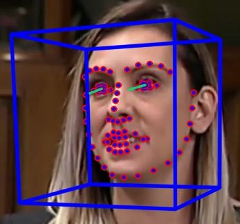
Introduction
The study of political speeches has too often been a missed opportunity. While political science
experienced a recent surge in the development of research methods based on text documents,
the textual record of political speeches represents only a tiny fraction of the data made available
to the research community every day. To gain an appreciation of this information loss, consider
President Obama’s famous statement at the 2004 Democratic National Convention: “There’s not
a liberal America and a conservative America; there’s the United States of America.” Using a
modern encoding standard, the transcript of this sentence represents about 96 bytes of data. The
corresponding audio track makes 200 thousand bytes. Its video signal, without sound, around
one million bytes.1 The reach of textual analysis, roughly speaking, sums up to less than 0.01
percent of the total quantity of data encoded in a typical video. More importantly perhaps, in
our example, the textual transcript would fail to translate many of the contextual clues—the tone,
pace, and gestures—that made Obama’s statement memorable.
    In this paper, we examine the performance of three modes of inquiry—text-as-data, audio-
as-data, and image-as-data—for the task of automated emotion recognition. For this purpose, we
introduce a novel collection of political videos containing sentence-long utterances from more
than 500 politicians in two different countries (Canada and the United States), recorded in various
contexts, and labeled by human coders for their emotional content. Our coding scheme comprises
two primary dimensions of affect, emotional arousal (or activation) and valence, as well as a
specific emotion of theoretical importance for political research—anxiety. We rely on machine
learning to compare the predictive power of each type of data input, and assess their potential
for empirical research in the domain of politics.
    Our study makes several contributions that may help inform future research in multimodal
analysis. First, our results validate recent claims that audio and visual signals can enhance the
automated analysis of political content, beyond what is feasible using textual transcripts (see e.g.
Dietrich, Enos, and Sen 2019; Dietrich, Hayes, and O’Brien 2019; Knox and Lucas 2018; Hwang,
Imai, and Tarr 2019; Torres 2018). We show that text-as-data is reliable for quantifying emo-
tional valence (positive versus negative sentiment) in political speech, while audio signals are
particularly useful for improving the levels of predictive accuracy in the modeling of activation
and anxiety. Second, we introduce a model of speech emotion recognition that relies on path-
breaking advances in voice synthesis to account for discrepancies in individual speaking styles.
Our approach, which can be adapted to a variety of deep learning architectures, relies on abstract
representations of a speaker’s voice, which we refer to as speaker embeddings. These embeddings
can be computed when making predictions for speakers not observed during the training stage,
and offer improvements in accuracy. Third, we address some of the difficulties involved in the
   1
     These calculations compare the text digitized in Unicode characters with the UFT-8 standard, an audio waveform
in 16 bit encoding at a 16,000 sampling rate, and a video format with a 720 pixel height at 30 frames per second.

                                                        1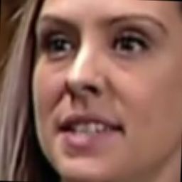
processing of visual data, an area of political methodology that is sure to grow in importance
in the discipline. We build upon modern tools from the field of computer vision to extract face-
centered images from our video collection, and show that deep convolutional networks based on
these visual signals can match the predictive accuracy achieved with either text or audio data.
    The following section begins with a survey of recent contributions from the field of political
methodology, before moving to theoretical considerations in the study of emotion. We then
introduce our corpus of videos, and present the modeling strategies that we considered for each
of the three modalities under scrutiny. The penultimate section reports our empirical results,
followed by a final discussion of the relative strengths of each modality.

The Automated Study of Emotion in Political Science
Our focus on emotion recognition in this paper is motivated by the current gulf between theo-
retical ambitions on the topic and the methods available to fulfill them. Studying the limits of
rationality and the role of emotions in human behavior is one of political science’s core research
agendas, and there is now a vast literature linking emotion to disparate outcomes such as the
formation of policy preferences, voting, election campaigning and messaging, responses to war
and terrorism, and social movement organization (for a review, see Brader and Marcus 2013). Yet
enthusiasm for this field of research is beset by the challenges involved in measuring emotions
accurately. In spite of the spectacular advances in the field of artificial intelligence, there are
still very few (if any) real-world applications able to detect and respond to our emotions (see
Schuller 2018). The slow pace of progress is a testament to the difficulty of the task. As noted
by Knox and Lucas (2018), the challenge is likely compounded when studying political elites,
who often exercise considerable emotional control over their speech, as compared to everyday
conversations.
     The branch of methodological research that has witnessed the most steady progress in this
area is textual analysis. Researchers have applied both dictionary-based and supervised learning
methods for sentiment analysis to a wide array of text documents pertaining to politics, from
politically-oriented social media tweets on the Twitter platform (Bollen, Mao, and Pepe 2011;
Mohammad et al. 2015), to records of parliamentary debates dating back to the early 20th century
(Rheault et al. 2016).2 Most instances of political communication, however, are not generated in
textual format; legislative proceedings, campaign debates, and other key speeches by political
actors are generally first delivered in spoken form. Consequently, scholars applying sentiment
analysis to political speeches are most often working with textual transcriptions of originally
spoken word. As illustrated with the example utterance in our introduction, by studying only
   2
    For more general overviews of the political literature in text-as-data, see Grimmer and Stewart (2013), Wilkerson
and Casas (2017), and Benoit (2019).

                                                         2
the textual transcriptions of such events, a large proportion of the available data remains hidden
from view.
Recognizing these limitations, a recent body of work has begun to explore how audio and/or
visual data might contribute to the better modeling of affect in politics. Dietrich, Enos, and Sen
(2019) and Knox and Lucas (2018) use novel techniques for audio data to study oral arguments
before the U.S. Supreme Court, showing that acoustic signals provide information about Justices’
emotional states and attitudes that is inaccessible using textual transcripts alone. Dietrich, Hayes,
and O’Brien (2019) have recently extended the analysis of acoustic signals to U.S. Congressional
floor debates, demonstrating how changes in vocal pitch relative to a speaker’s base level can
provide information about legislators’ broader issue positions. But for a few studies, audio signal
processing—now commonly used for emotion recognition in disciplines such as engineering and
computer science (see El Ayadi, Kamel, and Karray 2011; Poria et al. 2018; Schuller 2018)—has
been little integrated into the study of emotion in political science.
Political scientists have also been tentative in their adoption of automated methods using the
visual signal to study affect. In this case, the sheer volume of data encoded in videos poses an
additional burden in terms of computing time. Yet, as Torres (2018) points out, humans process
information in the world first with their eyes, responding emotionally to visual stimuli before
consciously processing what they see. Torres (2018) uses computer vision and image retrieval
techniques drawn from computer science to show that conservative and liberal media outlets por-
tray protest movements in visually disparate ways, with conservative outlets reporting protests
as more dangerous (associated with darker and more nocturnal settings) than liberal outlets. Re-
cent work by Hwang, Imai, and Tarr (2019) also applies computer vision techniques to political
science, using these methods to automate the coding of politically-salient variables in campaign
advertisement videos, an endeavor with promising implications for applied research.
The Representation of Emotions
This section provides a brief review of the two most widely adopted approaches for representing
emotions in computational studies, namely Ekman’s (1999) model of six basic emotions and the
related facial action coding system (FACS) (Ekman and Friesen 1971; 1978), and Russell’s (1980)
circumplex model of affect.3 We argue that the former suffers from shortcomings for applications
in political research, even though the FACS itself provides a useful starting point for develop-
ing models based on visual data. Next, we identify the visual and acoustic traits that may help
guide the process of feature engineering in automated speech recognition, and conclude with a
discussion of theoretical studies on anxiety.
3
An alternative choice is Plutchik’s (1980) wheel of emotions, used for instance by Mohammad, Kiritchenko, and
Zhu (2013), which we do not cover for simplicity.
3Our natural starting point is the psychological literature on emotions. Psychologists have
proposed a number of different approaches to classifying human emotion, with the most common
being either categorical or dimensional (Cambria, Livingstone, and Hussain 2012). Categorical
models of emotion are often underpinned by the idea that there are a series of “basic” or primary
emotions that underpin human emotional life. Of these, Ekman’s (1999) model of the six basic
emotions—sadness, happiness, surprise, disgust, anger, and fear—is a common choice in many
studies in speech emotion recognition. According to Ekman and Friesen (1971; 1978), these six
emotions are universal to human beings, and can be found across cultures. More controversially,
some scholars suggest that all other emotions emerge out of mixing these primary emotions
(Cowie and Cornelius 2003). Ekman and contributors also pioneered the Facial Action Coding
System (FACS), an exhaustive categorization of muscles movements occurring in various regions
of the face, which can be used to map a wide range of reactions to stimuli extending beyond the
six basic emotions (Ekman and Friesen 1978).
While the FACS appears indeed useful for guiding research based on visual data, the basic
emotions categorization is problematic for political research applications. Simply put, we find
that few of these six emotions are common in political videos. To demonstrate this point, ap-
proximately 1,400 video utterances from our datasets, which we discuss in greater detail in the
next section, were annotated for basic emotions. The emotion most frequently observed by our
human coders—anger—appeared in fewer than 14 per cent of these videos. Other basic emotions
were virtually never observed (for example, surprise, sadness or disgust), such that we would
require overly large collections of data before they could be considered in the development of
machine learning applications. In contrast, more than one third of the speakers in our videos
were coded as anxious, and even more were coded as emotionally aroused. Manifestations of
emotions are indeed frequent in political speeches, but they do not seem to fit easily in the six
basic categories. Our empirical analysis provides additional evidence to assess this specific point
on measurement.
A second theoretical approach to emotion representation is dimensional, perhaps best exem-
plified by Russell’s (1980) circumplex model. Dimensional approaches suggest that emotions can
be mapped onto a finite number of dimensions. Although models with varying numbers of di-
mensions have been proposed, the two-dimensional representation—valence and activation—is
often retained in computational studies (Fernandez 2004). Activation is a measure of emotional
arousal, the amount of energy involved in expressing an emotion (El Ayadi, Kamel, and Kar-
ray 2011). Valence (often called sentiment) refers to the negative or positive orientation of the
emotion being expressed. Discrete emotions can be placed along the continuum of these two
dimensions. Figure A1 in this paper’s Appendix reproduces Russell’s two-dimensional model,
and shows where some of the aforementioned basic emotions are located on each dimension.
In this model, anxiety (the emotional response to stress) is located in the upper-left quadrant,
4associated with emotional arousal and negative sentiment. This position is consistent with the
empirical correlations observed in our dataset and a body of literature focusing on anxiety (see
e.g. Gray and McNaughton 2000; Marcus, Neuman, and MacKuen 2000, Ch. 2).
Both the activation and valence dimensions of emotion have distinct manifestations in hu-
mans that allow us to form expectations for our three data modalities—textual, audio, and vi-
sual. Activation is often associated with measurable physiological changes that we expect audio
recordings of speech to best capture. When humans are activated, the sympathetic nervous sys-
tem becomes aroused. Heart rate and blood pressure increase, and respiration becomes deeper
(Williams and Stevens 1972). Other physiological changes such as mouth dryness or muscle
tremors may also be present. This triggers speech that is louder, faster, and “enunciated with
strong high-frequency energy, a higher average pitch, and wider pitch range” (El Ayadi, Kamel,
and Karray 2011, 573). Conversely, when de-activated, the parasympathetic nervous system dom-
inates, which slows heart rate and blood pressure. The result is speech that is relented, lower in
pitch, and with reduced high frequency energy (El Ayadi, Kamel, and Karray 2011).
While it may be well captured in acoustic signals, activation alone does not allow for differ-
entiation among discrete emotions. For instance, happiness and anger are both associated with
high arousal, and similar acoustic information (Sobin and Alpert 1999). The second “valence”
dimension, which measures whether an emotion is positive or negative, is also important for
classifying emotion. Unlike for activation, the positive/negative sentiment of a speech utterance
is likely to be discernible from the linguistic message of the speaker. Consider, for example, that
a textual transcript as short as President Obama’s “yes we can” refrain provides the information
needed to recognize that his message is positive. As discussed in previous sections, the ability of
textual data to capture valence is demonstrated in the success that scholars have had in harness-
ing these methods to measure negative/positive sentiment in a variety of textual data relevant
to politics.
Finally, there is a strong theoretical basis for using the visual signal contained in political
videos. The human face is the primary visual cue in human interaction (Harrigan and O’Connell
1996), and there is now a well-established literature showing that human emotions can be iden-
tified through the muscular activity of the face. Brief changes in facial appearance, such as the
raising of a brow, wrinkling of the nose, or puckering of the lips, combine to create the expres-
sion of different emotions (Ekman and Friesen 1978; Ekman and Rosenberg 2005). An emotion
with a negative valence such as fear, for example, is associated with a raised and straightened
eyebrow, open eyes, and dropped jaw (though the face may also be in a neutral position). For
disgust, the upper lip will appear raised, changing the appearance of the nose; and the cheeks
will be raised, causing lines below the eyes (Ekman and Friesen 1978). Even when choosing to
rely on a dimensional representation of emotions, these visual features should prove particularly
helpful to associate images with the target classes.
5The Special Case of Anxiety
In addition to the two dimensions discussed in the previous section, our study also considers
anxiety as a discrete emotion category. This emotion has arguably generated the most extensive
literature in political science, due to its prevalence and implications for decision-making behav-
ior. In particular, scholars have linked anxiety to a wide range of political phenomena, including
terrorism and foreign policy decisions (Huddy, Feldman, and Weber 2007; Rheault 2016), nega-
tive attitudes toward immigration (Brader, Valentino, and Suhay 2008), partisanship defection in
voting, and ethnic cleansing and genocide (Marcus, Neuman, and MacKuen 2000).
Anxiety is closely related to fear, yet the two expressions refer to different concepts. Freud
(1920) was among the first to establish this distinction; whereas fear is a response to immediate
and present danger, anxiety is a more generalized feeling of concern about “potential, signaled,
or ambiguous threat” (Blanchard et al. 2008, 3). Therefore, in a literal sense, we should not expect
politicians to experience fear, unless perhaps they are faced with a sudden and unexpected danger
(for instance, if a natural disaster or an active gunman disrupts their speech). Although the terms
are often conflated in common usage, more often than not, when we speak of fear in politics, we
actually mean anxiety.
Anxiety in the human voice should be closely associated with emotional activation. As is
true for emotional arousal, the sympathetic nervous system becomes activated when a person is
anxious (Harrigan and O’Connell 1996). Studies examining the acoustic correlates of fear, anxi-
ety’s most closely related emotion, show that this emotion is characterized by an increased pitch,
greater pitch variance, and a faster speech rate (Sobin and Alpert 1999; Banse and Scherer 1996).
However, these acoustic characteristics are also found in other emotions related to activation. A
study by Sobin and Alpert (1999), for example, shows that fear and anger share all but two acous-
tic features, which poses a challenge for multi-class problems in speech emotion recognition. The
same authors show that, as compared to other basic emotions, acoustic indicators appear to be
less important for human listeners in identifying fear in speech.
Facial traits should also provide useful reference points when modeling anxiety with visual
signals. Harrigan and O’Connell (1996) examined the correlates between facial features (includ-
ing the FACS discussed above) and human-coded annotations of anxiety in video recordings of
experimental subjects. They report that facial expressions related to the partial (rather than full)
expression of fear are visible on the faces of anxious speakers. These facial muscle movements
include the horizontal pulling of the mouth, raising of the brows, and an increased rate of blink-
ing. Meanwhile, facial expression associated with the more acute expressions of fear, such as
wide eyes, and more pronounced brow raising, were not observable in the videotapes. These
previous findings suggest that visual clues can be particularly helpful in differentiating anxiety,
not just from other emotions, but from fear as well.
6Video Collection
This study relies on three datasets of political videos annotated for their emotional content. The
first dataset contains just under 1,000 utterances spoken by Members of Parliament during Ques-
tion Period in the Canadian House of Commons (Cochrane et al. 2019). To build the corpus,
researchers at the University of Toronto randomly selected ten time points from every third
Question Period between January 2015 and December 2017. Video snippets were cut around
each time point to include a full sentence, using punctuation marks from the official transcripts
of the debates. Three independent coders watched and annotated the video clips for both va-
lence and activation on 0-10 scales, with 10 being the most positive valence, and most activated.4
For consistency with the rest of our video collection, we recoded valence and activation into bi-
nary 0-1 variables from the average coder score computed on the original 11-point scale. In this
first dataset, approximately 33 percent of utterances were labeled as activated, while 67 percent
were annotated as not-activated. For valence, 61 percent of videos were annotated as conveying
negative sentiment, while 39 percent were coded as conveying positive sentiment.
The second dataset, collected in the spring of 2019, contains 1,000 video utterances selected at
random from three sources: a collection of all Question Periods in the Canadian House of Com-
mons between January 2015 and December 2017 (the original, full-length collection of videos
described above); a collection of all floor proceedings from the United States House of Represen-
tatives between March 21st , 2017 and May 23rd ; and, the 30 most watched hearings of the Senate
Judiciary Committee posted by CSPAN between January 2015 and June 2019. We relied on a
custom script to detect silences and randomly select segments between 5 and 20 seconds—the
average duration of a sentence being 10 seconds. Videos were then individually inspected to dis-
card segments with multiple speakers. Each video was labeled by three annotators for valence,
activation, and anxiety on Amazon MTurk’s crowdsourcing platform. To improve the quality
of our annotations, we restricted the task to workers with a “Master’s” badge, indicating a high
rate of approval on the site. In this second dataset, about 35 percent of videos were labeled as
activated, and 65 percent were coded as non-activated. 62.5 percent of videos were annotated
as conveying a negative sentiment, while 37.5 percent were annotated as conveying a positive
sentiment. Anxiety was present in 33 percent of videos.
We collected our third dataset in the summer of 2019. In contrast to the first two, the purpose
of this dataset was to oversample speeches from specific politicians to further examine the con-
sequences of speaker heterogeneity in speech emotion recognition tasks. As a result, we created
this dataset by manually curating a list of recent speeches from ten high-profile political actors,
five men and five women (see Table 3 for included speakers). This selection method is admit-
tedly not as robust as random sampling (the availability of videos may be determined by media
4
Three separate coders also annotated textual transcriptions of the data, but we do not draw on these annotations
in this study. These videos were also labeled for the six basic emotions categories.
7coverage choices), but it allowed us to accumulate extended examples from prominent speakers.
Just over 1000 utterances—approximately 100 videos for each speaker—were compiled, selected
from videos that were openly available in high resolution on the YouTube platform. Each video
was once again annotated by three workers on the MTurk crowdsourcing platform. Consistent
with the distributions observed in the previous two datasets, 36 percent of videos were labeled as
activated. For valence, 60 percent of videos were coded as conveying negative sentiment, while
40 percent were coded as conveying positive sentiment. Annotators marked the speaker as anx-
ious in 30 percent of the videos. In total, the three datasets comprise 2,982 video utterances with
emotion annotations, and featuring 502 different political actors.
Methods
This section introduces the principal concepts and models used to process the three modalities at
the core of this project: text-as-data, audio-as-data, and image-as-data. We use the term “modal-
ity” when referring to each communication channel, following the terminology used in other
disciplines (see e.g. Baltrušaitis, Ahuja, and Morency 2018). We start by introducing the textual
models that we use as a basis for empirical comparisons, although this discussion is deliberately
brief given the breadth of literature already available on this modality. Next, we discuss the mod-
eling of audio signals and describe the challenges involved with speech emotion recognition, in
particular speaker heterogeneity. We then outline the methodology that we propose to address
some of these difficulties. Finally, we repeat these steps for the visual modality.
Text Modality
Our empirical analysis starts by establishing a benchmark for the accuracy of emotion recogni-
tion models using textual input.5 We fit machine learning classifiers on the text from each video
utterance in our collection, using the three emotion labels described in the previous section. We
rely on a methodology that had long represented the state of the art for text classification, namely
long short-term memory (LSTM) recurrent neural networks fitted on sequences of tokens con-
verted into numerical vectors using pre-trained word embeddings. The latest trend in the field is
to rely on transfer learning using base models accounting for more complex linguistic structures
(see, for example, Devlin et al. 2018; Howard and Ruder 2018). For simplicity, we report results
only with the first approach.
Our classifiers rely on word embeddings computed using the GloVe algorithm (Pennington,
Socher, and Manning 2014) to convert each word into numerical vectors of dimension M =
5
We retrieved the textual content of videos from the last two of our datasets using the Google Cloud Speech-
to-Text API. The model adapted for video recordings generates transcriptions of high fidelity, and its extensive
dictionary helped to identify proper nouns, even challenging ones, such as the names of electoral districts and
foreign politicians.
8300. We use padding to normalize each utterance to T tokens. As a result, each input in the
classifier is encoded as a T × M tensor. Given the short size of each utterance, we did not apply
text preprocessing. Natural language being organized as sequences of words, recurrent neural
networks (RNNs) represent a natural choice as they are capable of learning from current and
previous elements in a sequence (Goodfellow, Bengio, and Courville 2016, Ch. 10). Specifically,
we rely on LSTM networks, which include a “memory cell” that learns to either remember or
forget prior contextual information associated with inputs as information moves through the
network (see Greff et al. 2016). Our empirical section reports results from classifiers with an
identical architecture for the three emotion labels, using two LSTM layers with 100 and 50 nodes
followed by two dense layers.
Audio Modality
Digital audio signals are a data type that differs from the typical input formats used in social sci-
ence research. As a result, we start with a brief introduction of three concepts: the speech signal,
the waveform, and spectral analysis. Next, we address the question of speaker heterogeneity—the
presence of repeated instances of the same speakers in a dataset—and propose a novel method-
ology to account for differences in the baseline voice patterns of each speaker. We conclude with
a summary of the proposed model architecture for the audio modality.
A speech signal—like the sound of a voice in a natural environment—is produced through
vibrations, or cyclical patterns occurring rapidly over time (see Rabiner and Schafer 2011, Ch. 1).
Relevant for the following discussion is the fact that higher sounds are produced with faster vi-
brations, hence more cycles per seconds. The number of cycles per second is called the frequency
and is measured in hertz (Hz). Thus, a politician with a higher pitch speaks at a higher base fre-
quency. Louder sounds, on the other hand, produce larger waves for a given frequency. This is
the amplitude, measured for instance in decibels. Because of the digital conversion of natural
sound, the units of measurement for amplitude are not always preserved on a known scale of
reference—volume can be adjusted, amplifying all waves, or mixed to amplify/attenuate sounds
in specific ranges of frequencies (see Boersma 2014, 379). What matters for the purposes of signal
processing is that higher amplitudes be measured with larger numbers, regardless of the scale.
A central technology involved in sound recording converts the air pressure waves to an elec-
tric signal, called the waveform (Rabiner and Schafer 2011; Boersma 2014). The raw waveform is
a unidimensional array of integers—the encoding in our set of videos uses a signed, 16-bit inte-
gers format—where each number represents the amplitude in discrete time. The sampling rate,
also measured in hertz, is the frequency at which each integer is recorded.6 With a sufficiently
6
Modern videos typically have sampling rates of 44,100 or 48,000 Hz that can be recorded simultaneously on
different channels (e.g. two in the case of stereo recordings). For our analyses, we convert the sample rate to 16,000
Hz and use a single channel.
9high sampling rate, the waveform can reproduce accurately the pulses of air pressure as they
occur in the original speech signal. Figure 1a depicts the raw waveform of a speech from our
dataset, a ten-second utterance from Barack Obama during the third 2012 presidential debate.
Noticeable are the frequent pauses characteristic of Obama’s speech pattern, during which the
vibrations stop. Since the signal was converted to a 16KHz sampling rate, there are 16,000 data
points every second; zooming in on parts of this figure would reveal elaborate patterns of pulses
representing the various vocal sounds produced when uttering words.7
Figure 1: Digital Signal Processing of a Recorded Sentence from Barack Obama
(a) Waveform (b) Frequency Spectrum
(c) Spectrogram
The last building block in audio processing is spectral analysis, which includes various ways
to express the waveform in the frequency domain. The aim is to represent sound amplitudes
as a function of each frequency, usually with Fourier transforms (Boersma 2014). The resulting
spectrum (or periodogram) helps us to understand which frequency ranges characterize a par-
ticular speech signal, for instance whether a speaker tends to produce sound at higher or lower
frequencies. Figure 1b is the frequency spectrum of the aforementioned utterance from Barack
Obama, computed with a Hamming window and displaying positive values in the 75 to 300Hz
range. The first observable peak is the fundamental frequency, which corresponds to perceived
pitch, and is followed by harmonics across the rest of the frequency range (Rabiner and Schafer
2011, Ch. 10). An additional transformation is the spectrogram (illustrated in Figure 1c for the
7
The study of such patterns is the field of phonetics, a topic addressed in more depth elsewhere (see e.g. Laver
1994; Boersma 2014).
10same example), which converts back the frequency spectrum in the time domain. The spectro-
gram depicts time on the x-axis, frequencies on the y-axis, and amplitudes using a color code.
Our audio signal models rely on features derived from the waveform and from methods for spec-
tral analysis. The most common audio feature for machine learning is the mel-frequency cepstral
coefficients (MFCC), which are calculated by further transforming the audio spectrum (see, e.g.
Zheng, Zhang, and Song 2001).
Dealing with Speaker Heterogeneity
Acoustic signals from political speeches should contain many clues revealing emotional states,
but their analysis causes complications due to the distinctiveness of each voice. This problem par-
allels the heterogeneity biases that may arise in inferential statistics when dealing with panel or
hierarchical data. For example, without any correction, estimating changes in pitch as a measure
of emotional activation makes sense for comparisons based on samples from the same speaker.
However, every voice being unique, the pitch of an emotionally subdued person may fall just
about anywhere in comparison to that of a second, emotionally aroused speaker. To address this
problem, Dietrich, Hayes, and O’Brien (2019) relied on measurements of the baseline pitch level
for each of the speakers in their dataset, before normalizing relative to the baseline. In effect, this
achieves a similar goal as the within transformation in panel data analysis, where group-level
means are subtracted from the variables. As far as we can tell, many applications of speech emo-
tion recognition have simply ignored the presence of repeated examples from the same speakers
in the training data.
We illustrate this problem by comparing the periodograms of female and male speakers in
the first of our datasets. The plots in Figure 2 take advantage of the additive property of Fourier
transforms and the randomized selection procedure to compute bootstrapped estimates of the
average spectrum for subgroups of speakers. Such techniques are commonly used for spectral
analysis in other disciplines (see, for example, Zoubir and Iskander 2004). The Figure illustrates
average differences in frequencies between activated and calm speakers, broken down by gen-
der. As can be observed, while the typical voice of politicians from either gender is transformed
when emotionally activated, the voices of women and men also exhibit different patterns. For
men, a range of low to mid-level frequencies have a higher amplitude when emotionally aroused,
whereas the change tends to occur in higher frequencies for women. This suggests that emotions
alter the timbre—or the range of harmonics—heterogeneously across groups of speakers. As a
result, without knowing the gender of speakers a priori, predictive models are already at risk of
confounding this attribute with the variation associated with emotions. Consider the extreme
case of a sample in which speakers from a given gender are observed for only one emotional cat-
egory; a classifier may learn to predict emotions based on the gendered attributes of a voice, and
11predictions made on new data would reproduce the bias that was present in the training data.8
Gender, however, is not the only source of ambiguity in audio data. Heterogeneity originates to
a large extent at the level of individual speakers, and may be caused by other contextual factors
at the time of recording.
Figure 2: Activated vs Subdued Speakers, by Gender (Frequency Domain)
(a) Women (b) Men
Activated Activated
40 Calm Calm
30
25
30
20
Amplitude
Amplitude
20
15
10
10
5
0 0
0 100 200 300 400 500 600 700 0 100 200 300 400 500 600 700
Frequency (Hz) Frequency (Hz)
Mean frequency spectrum by groups of speakers for the audio samples in our first dataset from the Canadian
House of Commons, computed using a bandpass filter to attenuate frequencies outside the 100-500 Hz range. The
outermost error bands represent 95% bootstrap confidence intervals.
Our approach builds on methods developed in the field of automated speaker recognition
(ASR), which is concerned with identifying the voice profiles of speakers. Early techniques in
ASR include cepstral mean and variance normalization, which consists of centering the features
extracted from each audio waveform (Viikki and Laurila 1998). Normalizing the acoustic features
was found to improve predictive performance by eliminating noise associated with the recording
conditions of the original speech signal. Applying a similar transformation at the speaker level
before fitting a predictive model would be one possible way to deal with heterogeneity, and
amounts to extending Dietrich et al.’s approach of normalizing the pitch of speakers to a broader
range of mel-frequency cepstral coefficients. Modern approaches in ASR have led to alternatives
such as i-vectors and x-vectors, embeddings representing the properties of a voice, which are
commonly used in tasks such as speaker diarization (Snyder et al. 2018).
The method that we propose to deal with heterogeneity relies on the embeddings from a voice
encoder, which we have found to generate surprisingly efficient representations of politicians’
voices. These embeddings have been originally developed for speech synthesis, and correspond
to the output layer of pre-trained models designed for speaker identification (the implementa-
tion we rely on is described in Wan et al. 2018; Jia et al. 2018).9 This model has served as a
8
A stream of research has emphasized the existence of similar biases caused by the choice of training samples
(Caliskan, Bryson, and Narayanan 2017). In inferential statistics, we would also speak of an omitted variable bias in
the previous example.
9
The source code and pre-trained models we used are released in the following repository:
12building block for text-to-speech applications such as Google’s Tacotron (Jia et al. 2018). Our
implementation relies on models trained using data from the LibriSpeech (Panayotov et al. 2015)
and VoxCeleb (Chung, Nagrani, and Zisserman 2018) corpora, primarily designed for the devel-
opment of speaker recognition machines.
Our approach consists of using the combined audio of all speeches available for each speaker
in our dataset to compute what we call speaker embeddings, an abstract numerical representa-
tion of each speaker’s voice.10 We use the pre-trained weights of the voice encoder described
above to generate embeddings of 256 numbers. Figure 3 plots these embeddings for two politi-
cians using a two-dimensional heatmap to illustrate the methodology. The subtle differences in
values reflect the idiosyncratic traits of each voice. Our goal is to augment predictive models
of speech emotion recognition using these speaker embeddings, hence accounting for for the
baseline voices of politicians. Again, a parallel can be made with models in inferential statistics
that include unit-specific intercepts (e.g. fixed or random effects), with the difference that these
speaker embeddings are continuous-valued and multidimensional.
Figure 3: Examples of Speaker Embeddings
(a) Barack Obama (b) Elizabeth Warren
0.200
0.175 0.20
0.150
0.125 0.15
0.100
0.10
0.075
0.050 0.05
0.025
0.000 0.00
Visualizations of two speaker embeddings using a heatmap. Each embedding is an abstract summary of the unique
identifiers associated with a speaker’s voice.
To assess the face validity of this approach, we plot the generated speaker embeddings on
two dimensions using principal components analysis, and report the results in Figure 4. We use
a color code to distinguish between male and female speakers. The projection reveals how these
embeddings properly distinguish between female and male voices, each being clustered together
in one region of the figure.11 More generally, speakers with similar voices will be located closer
together in the vector space.
https://github.com/CorentinJ/Real-Time-Voice-Cloning.
10
We also verified that these speaker embeddings do not retain emotional characteristics per se, by computing
them on a separate training set and making predictions on a holdout set. For simplicity, we report only of set of
results in this study. In fact, the voice encoder requires only a relatively short sample of each speaker’s voice to
generate reliable embeddings.
11
The female voices closer to the male cluster are deeper voices with more “masculine” traits, and vice-versa.
13Figure 4: Projections of Speaker Embeddings in the Consolidated Dataset
0.4 Women
Men
0.3
0.2
Second principal component
0.1
0.0
−0.1
−0.2
−0.3
−0.4 −0.2 0.0 0.2 0.4
First principal component
Distribution of all speaker embeddings in a two-dimensional space using principal components analysis. Voices
from the same gender tend to resemble each other and are clustered together in the vector space.
The benefits of this approach are threefold. First, the embeddings can be generated for new
examples, never seen before during the training stage of an emotion recognition application.
Indeed, the voice encoder can be applied to any new speaker using a sample of their voice.
An emotion recognition model trained with a sufficient number of examples can then rely on
learned information about speakers with similar voices to predict the emotional state of new
speakers more accurately. Second, the embeddings account not only for individual baselines, but
also for other attributes that may affect predictive accuracy, for instance gender. Third, these
speaker embeddings offer a lot of flexibility: they can perform the same purpose—speaker-level
normalization—using other modalities since they are unique to each speaker, and be reshaped in
different ways to match the input size of neural network layers.
Finally, we implement our methodology using a neural network architecture for speech emo-
tion recognition in which acoustic features are augmented with these speaker embeddings. We
depict this architecture in Figure 5. The first stage involves converting the waveform input of a
speech into an array of features, which is then concatenated with the speaker embedding for the
particular politician uttering that speech. Features are extracted from the waveform from each
14audio file. For this paper, we rely on the full set of 68 mid-term audio features computed using
the pyAudioAnalysis library (Giannakopoulos 2015) applied to non-overlapping windows of 0.25
seconds. The concatenated array of features constitutes the input of a multilayer perceptron,
with the output layer being the emotional class that we aim to predict.
Figure 5: Emotion Recognition with Speaker Embedding
Audio Features
(e.g. MFCC) Feedforward Network
Audio Signal
Output Node
Speaker Embedding
Schematic depiction of a deep neural network for speech emotion recognition, including speaker embeddings
concatenated with the input features.
Visual Modality
This section introduces the visual models used to complete our analysis. We start with a dis-
cussion of computer vision toolkits available to preprocess images and locate the face of each
politician in the video collection. We argue that this stage serves an important purpose by re-
ducing extraneous elements from the frame. Next, we discuss the selection of a deep learning
architecture appropriate for images, which have a different shape than the data types associated
with the previous modalities.
Ignoring sound, a video is just a rapid sequence of images—or frames—chronologically ap-
pended together. Similar to digital waveforms, the visual signal is recorded at a variable sampling
rate representing the number of frames captured per second. This rate is usually around 30 frames
per second in modern standard formats found on the web. The dimensions of each frame, the
resolution, may vary and affect the quality of the recording. Most of our videos, with the ex-
ception of the HouseLive collection, have a width of 1280 and a height of 720 pixels, a common
15resolution for high definition videos. Thus, each frame in the video file is a multidimensional
array (or tensor) of integer values with dimensions width × height × channels. The channels are
the three basic colors, or put another way, each pixel is represented by a tuple of three integer
values corresponding to red, green and blue.
Many open libraries from the field of computer vision facilitate the processing of video sig-
nals. Existing models have become spectacularly efficient for tasks such as face recognition and
facial landmark detection, which offers a useful entry point for advancing research based on vi-
sual data in political science. In particular, we rely heavily on face recognition to process our
videos. The external tools for this task depend on two core libraries in computer vision: OpenCV
and dlib. The latter is a general-purpose library for deep learning, which contains the source
code for our face recognition algorithm. Moreover, our empirical section briefly discusses facial
landmark features extracted using Baltrušaitis et al.’s (2018) OpenFace C++ library, which is itself
built on top of OpenCV and dlib.12
We choose to focus mainly on the face given the previously surveyed literature establishing a
relationship between facial features and human emotions (Harrigan and O’Connell 1996; Ekman
and Rosenberg 2005). Of course, there are several visual attributes of interest for speech emo-
tion recognition, such as hand gestures and other, non-face related corporal motion. Based on
observations made on our video collection, however, we argue that the face is a reliable starting
point for modeling political videos. Depending on the context—close-up shots, speaker standing
in front of a podium—the hands are often obstructed from view, whereas full body movements
are also constrained for speeches made from a seated position, as is the case, for example, in
Senate hearings. The face, on the other hand, is focused on systematically by camera workers.
Our main preprocessing step aims to identify and isolate the face of the speaker within the
frames of each video, to reduce other sources of noise. We did this by first collecting external
pictures of politicians in our dataset—in nearly all cases, using official portraits available on Cana-
dian and US parliamentary websites. Each picture serves as the target for face recognition. We
then processed each video using a face recognition algorithm from the dlib library,13 to match
faces present in each frame of our videos with the politician actually making the speech. The
library works by measuring the similarity of the encoding for a face detected in the video with
the encoding of the target image. This preprocessing step appears particularly important given
that many of our videos include multiple faces per frame. Without efforts invested in this disam-
biguation, the accuracy of learning models can be affected by extraneous information present in
the background of each video, which our coders were instructed not to consider. After a success-
ful match with the target face, we crop the frame to include only the target face, and create a new
12
The source code for all these models is released publicly, although OpenFace has restrictions for commercial
usage.
13
The algorithm was ported to Python and is available openly at: https://github.com/ageitgey/face recognition.
It achieves near perfect accuracy on benchmarks datasets for face recognition.
16Figure 6: Preprocessing Pipeline and Model Architecture for Visual Modality
Global Pooling
Input Video Face Recognition
(256 × 256 × 3) Top Layer
Output
InceptionV3
Speaker Embedding
Illustration of the face recognition stage and model architecture, with an example video for our corpus featuring
Canadian MP Ruth-Ellen Brosseau. Our main model uses the InceptionV3 ConvNet architecture (Szegedy et al.
2016), including a concatenation with speaker embeddings at the global pooling stage, and three additional dense
layers.
video, now resized to a constant 256 x 256 x 3 format. We perform this operation every tenth
frame, so that individual images can be used as input data while avoiding redundancies.14 Figure
6 illustrates this preprocessing technique with an actual example from a video in our corpus.
Since images are three-dimensional, we require a model adapted to this data format. We rely
on deep convolutional neural networks, specifically the modern Inception architecture proposed
by Szegedy et al. (2016), widely used for image processing tasks. We also consider the method-
ology introduced in the previous subsection—correcting for heterogeneity in the corpus—in this
case by concatenating the global pooling layer at the top of the Inception base module. We jux-
tapose three layers on the top of this architecture, plus an output layer using a sigmoid function
to predict the binary emotion classes. As we did with the audio data, we will compare results
achieved both with and without speaker embeddings. We use the embeddings discussed previ-
ously, based on voice recognition. Because they represent abstract numerical fingerprints, these
embeddings can be used for a similar objective by integrating a baseline for each politician in
the sample.15
14
At a rate of 30 frames per second, any pair of consecutive frames tends to be very similar.
15
We also computed visual speaker embeddings using the encodings from the above-mentioned face recognition
algorithm. For simplicity, we discuss only one sets of results in the next section.
17Finally, we rely on the the OpenFace toolkit mentioned earlier, as a validation probe to ex-
amine the association between facial features and emotions. The toolkit itself is based on deep
learning models in computer vision, trained to recognize facial landmarks as well as action units
from Ekman and Friesen’s (1978) coding system. The features extracted comprise the pose, glaze
direction, facial landmark location, and 18 action units from the FACS. Figure A2 in the appendix
illustrates the output of this feature extraction algorithm applied to one of our videos. This soft-
ware library appears particularly promising for applied research with image-as-data, although
we should note that it requires proper calibration to deal with noisier videos in which multiple
faces are present. Lower resolution videos also yielded problematic results. For this reason, our
main models do not include the OpenFace features, and we use them as a complementary source
of information to support our analysis in the next section.
Empirical Results
This section presents the key findings based on models fitted using each of the three data types,
following the same order as in the previous section. Starting with the textual modality allows
us to establish a frame of reference, although note that our main interest is in the improvements
achievable with the other two modalities. For each type of input data, we report accuracy results
for the main emotion classes: valence (or sentiment), activation, and the specific emotion of
anxiety. Finally, we discuss the key findings and compare the potential of each modality for
future research on political videos.
Text Models
The starting point for this paper was the observation that automated methods for emotion de-
tection using textual data are effective at extracting negative/positive sentiment, but less capable
of capturing other facets of emotion such as activation, and emotions related to activation. To
highlight this point, we fit models predicting sentiment, activation, and anxiety using the tex-
tual transcriptions of the speech snippets in our datasets. The models reported here use word
embeddings and recurrent neural networks, each with two long short-term memory layers (of
length 100 and 50, respectively). Models are fitted with the Adam optimizer (with a learning rate
of 0.001) over 15 epochs, such that the training corpus passes through the training examples 15
times. Regularization with dropout is used, with 1 in 5 neurons randomly removed from the
network during training, to avoid overfitting the model.
Table 1 reports cross-validation metrics for textual models of sentiment, activation, and anx-
iety in our datasets. Since we are dealing with unbalanced classes, we report the percentage of
observations in the modal category along with the accuracy score and the proportional reduc-
tion in error (PRE). Reported metrics are calculated on a holdout set representing 20 per cent
18of the overall dataset. As anticipated, they show that textual models make reasonable predic-
tions for sentiment—the models presented here accurately classified sentiment for 77 per cent
of documents, reaching a reduction in error of approximately 39 percent. Textual models for
activation and anxiety, meanwhile, perform poorly enough that guessing the modal category
would actually yield a better accuracy rate. We tested a number of parameterizations, but the
key substantive conclusion remains.
Table 1: Metrics for Textual Models
Emotion Accuracy(%) Modal Category(%) PRE (%)
Valence 77.2 62.5 39.3
Activation 64.5 67.3 –8.7
Anxiety 66.1 68.4 –7.7
These results confirm a driving hypothesis of this paper—that textual data is useful for detect-
ing negative/positive valence in text, but not the dimension of emotion associated with activa-
tion. This parallels recent findings in a study by Cochrane et al. (2019) that assessed the ability of
human coders to detect emotional content—sentiment and activation—in the written versus video
record of Canadian parliamentary debates. The authors show that human coders reliably agree
on the sentiment of an utterance, whether they watched the video or read the textual record.
In contrast, coders annotating activation from textual versus video records demonstrated little
consistency with one another. As Cochrane et al. (2019, 2) conclude, “in short, the sentiment of
the speech is in the transcript, but the emotional arousal is not.”
Audio Models
We now turn to the audio signal to asses whether information gains are feasible relative to models
based on text data. We begin by discussing associations between common audio signal features
and our emotion categories. Next, we provide a detailed illustration of the problem of hetero-
geneity in speech recognition. We start by fitting predictive models using a single speaker at a
time, and proceed by comparing these results with a pooled model, combining over 500 politi-
cians. Finally, we report results from our main model enriched with speaker embeddings, and
discuss the impact on predictive accuracy.
To begin, Table 2 reports average values of common acoustic features for each of the 2,982
speeches in our consolidated dataset, across the labels for activation and anxiety. We also report
difference in means t-tests along with their p-values. The features include the energy (the nor-
malized sum of squared values from the waveform); the pitch, or estimates of the fundamental
frequency, using two different toolkits; the pitch standard deviation; and the speech rate, mea-
19sured with the number of syllables over the speaking duration.16 For both activation and anxiety,
the differences are consistent with theoretical expectations. Activated and anxious politicians
speak with a higher pitch, a larger pitch variance, and slightly faster than confident speakers
(significantly so in the case of activation). Unsurprisingly, activated speakers produce more en-
ergy, meaning that they tend to generate a larger amplitude.
Table 2: Audio Features by Emotional Category
Feature Activated Calm t p-value
Energy 0.020 0.018 2.918 0.004
Pitch (Reaper) 189.527 154.971 21.038of each input, each of which is associated with the original label observed at the utterance level.
A similar approach has been used in learning tasks involving audio samples (see e.g. Hershey
et al. 2017). Table 3 reports the percentage of observations in the modal category along with
the accuracy score and the proportional reduction in error (PRE). Overall, when focusing on a
single speaker at a time, our models reduce the error rate by about 30% compared to guessing
the majority category.
Table 3: Accuracy Results for Speaker-Specific Models (Activation)
Politician Accuracy (%) Modal Category (%) PRE (%)
Alexandria Ocasio Cortez 74.6 61.5 34.0
Barack Obama 72.9 61.2 30.3
Brett Kavanaugh 82.4 76.4 25.8
Christine Blasey Ford 76.8 65.2 33.2
Donald Trump 72.3 61.2 28.5
Elizabeth Warren 76.6 64.8 33.6
Hillary Clinton 81.8 77.6 18.6
Jody Wilson Raybould 79.3 68.8 33.6
Justin Trudeau 80.4 69.6 35.4
Mitt Romney 72.2 61.1 28.4
Pooling all speakers together in the same model architecture results in a large drop in predic-
tive accuracy (see first rows of each panel of Table 4). We would normally expect the opposite,
since the pooled model contains many more training examples, which should improve the per-
formance of machine learning classifiers. Moreover, the model specification is identical to the
one used for individual speakers. Yet, accuracy drops under 70% for activation, with a modest 15%
reduction in error. This number is lower than the average of individual models reported in the
previous table. This result helps to emphasize one of the contentions made earlier regarding the
impact of speaker heterogeneity. Especially when models include multiple speakers, which will
often be the case in research on political videos—in our case, we have 502 different voices, most
of which appearing multiple times—accounting for heterogeneity appears desirable for training
reliable classifiers.
Table 4 contrasts the previous result with models concatenating speaker embeddings, as de-
scribed in the previous section. The rest of the model architecture is the same. For activation,
the inclusion of a speaker baseline increases the accuracy above the level achieved with sepa-
rate speakers. Model performance is also improved for anxiety, where the reduction in error
now reaches approximately 47%. These results also suggest that, contrary to models based on
textual data, audio signals perform better at detecting activated emotional states, as opposed to
21You can also read