Spatial parasite ecology and epidemiology: a review of methods and applications
←
→
Page content transcription
If your browser does not render page correctly, please read the page content below
1870

                 Spatial parasite ecology and epidemiology: a review of
                 methods and applications

                 RACHEL L. PULLAN 1 *, HUGH J. W. STURROCK 1 , RICARDO J. SOARES MAGALHÃES 2 ,
                 ARCHIE C. A. CLEMENTS 2 and SIMON J. BROOKER 1,3
                 1
                   Faculty of Infectious and Tropical Diseases, London School of Hygiene and Tropical Medicine, London, UK
                 2
                   School of Population Health, University of Queensland, Herston, Queensland, Australia
                 3
                   Kenya Medical Research Institute-Wellcome Trust Research Programme, Nairobi, Kenya

                 (Received 13 January 2012; revised 11 March 2012; accepted 3 April 2012; first published online 19 July 2012)

                 SUMMARY

                 The distributions of parasitic diseases are determined by complex factors, including many that are distributed in space.
                 A variety of statistical methods are now readily accessible to researchers providing opportunities for describing and
                 ultimately understanding and predicting spatial distributions. This review provides an overview of the spatial statistical
                 methods available to parasitologists, ecologists and epidemiologists and discusses how such methods have yielded new
                 insights into the ecology and epidemiology of infection and disease. The review is structured according to the three major
                 branches of spatial statistics: continuous spatial variation; discrete spatial variation; and spatial point processes.

                 Key words: Spatial epidemiology, parasites, spatial statistics, geostatistics, mapping.

                 INTRODUCTION                                                                        separately the three major branches of spatial
                                                                                                     statistics: continuous spatial variation; discrete spatial
                 Parasites are heterogeneously distributed within host
                                                                                                     variation; and spatial point processes (Cressie, 1991;
                 populations (Anderson and May, 1991; Anderson,
                                                                                                     Diggle, 1996).
                 1993). Usually, some of this heterogeneity will be
                 spatially structured and explained by various ecologi-
                 cal factors and species interactions that are themselves
                 spatially structured. Improved understanding of the                                 Approaches to spatial analysis
                 spatial patterns of infection and disease, and the pro-                             Any statistical approach that accounts for either
                 cesses behind them, can help predict spatial distri-                                absolute location and/or relative position (spatial
                 butions in unsampled areas, assist in the geographical                              arrangement) of the data can be referred to as spatial.
                 targeting of control interventions and improve our                                  There are three main approaches, illustrated in Fig. 1.
                 understanding of disease outbreaks.                                                 The feature that distinguishes between them is the
                    A number of tools are now available to help us                                   basic underlying statistical model, and the assump-
                 better quantify and understand spatial variation in                                 tions that this makes regarding the spatial processes
                 the patterns of infection and disease. The recent                                   involved (Diggle, 2004). For instance, spatial stat-
                 application of global positioning systems (GPS),                                    istics investigating continuous spatial dependency
                 geographical information systems (GIS) combined                                     assume that the outcome occurs and is potentially
                 with spatial statistical approaches, for example, has                               measurable throughout space and, as such, spatial
                 provided an improved understanding of spatial pat-                                  variation in the outcome can be modelled explicitly.
                 terns and processes (Hay et al. 2000; Simoonga et al.                               In contrast, discrete spatial statistics investigate
                 2009; Machault et al. 2011). This has, in turn, en-                                 proximity and are used when data are only available
                 abled us to predict spatial distributions using                                     at an aggregate area level. Here, spatial structure is
                 remotely sensed environmental data to assist the                                    modelled by considering dependency between neigh-
                 targeting of control and estimation of the burden of                                bouring discrete units. Both of these approaches
                 parasitic diseases (Brooker, 2007; Patil et al. 2011;                               rely upon spatially sampled measurement data, and
                 Soares Magalhães et al. 2011c). In this review, we aim                              can be described as global in the sense that they model
                 to provide an overview of available tools, methods                                  the overall degree of spatial autocorrelation for a
                 and their applications for improving our under-                                     dataset. Spatial point processes, on the other hand,
                 standing of the ecology and epidemiology of human                                   concern the physical location of events distributed
                 parasitic diseases. As a framework, we consider                                     within a study region and are used to investigate
                                                                                                     either the general (i.e. global) propensity for points
                 * Corresponding author: Dr Rachel Pullan. E-mail: rachel.                           to cluster or the location of individual (i.e. local)
                 pullan@lshtm.ac.uk                                                                  spatial clusters of infection, disease or vector and

                Parasitology (2012), 139, 1870–1887. © Cambridge University Press 2012. The online version of this article is published within an Open
                Access environment subject to the conditions of the Creative Commons Attribution-NonCommercial-ShareAlike licence < http://
                creativecommons.org/licenses/by-nc-sa/3.0/ > . The written permission of Cambridge University Press must be obtained for commercial re-use.
Downloaded from doi:10.1017/S0031182012000698
                https://www.cambridge.org/core. IP address: 46.4.80.155, on 30 Dec 2020 at 18:15:31, subject to the Cambridge Core terms of use, available at https://www.cambridge.org/core/terms
. https://doi.org/10.1017/S0031182012000698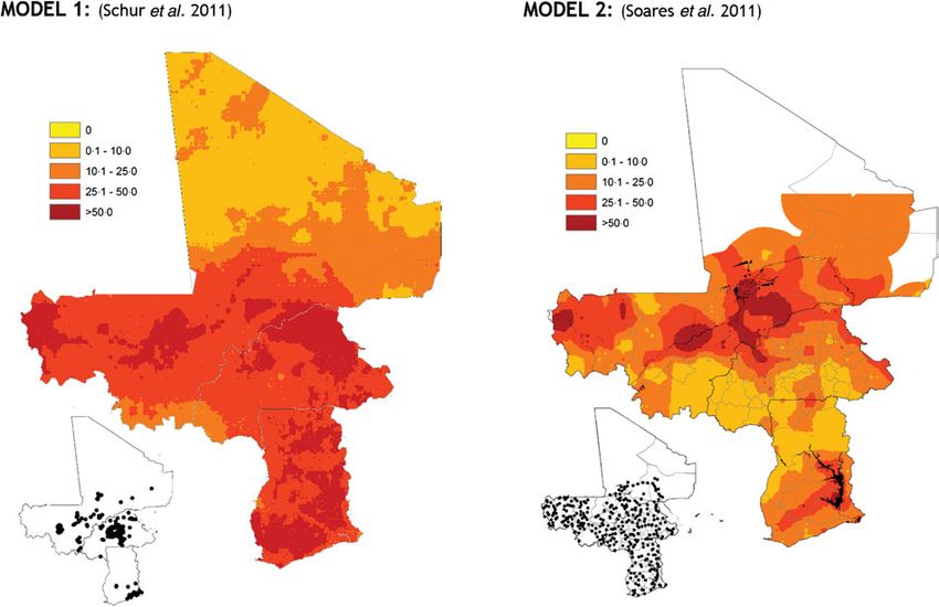
Spatial parasite ecology and epidemiology                                                                                                                  1871

            Fig. 1. An illustrated application of the three major branches of spatial statistics, using one dataset. (A) Data used for
            analysis: Point-level (school-level) malaria prevalence data for Western Kenya, collected during the National School
            Malaria Survey, 2010 (Gitonga et al. 2010). (B) Discrete spatial analysis: data are aggregated to the area level (in this
            case, mean district prevalence) for presentation and analysis. Discrete spatial statistics can be used to smooth between
            units, or investigate associations with covariates. (C) Continuous spatial analysis: characterizes spatial dependency (or
            autocorrelation) between points, and can be used to interpolate predicted outcomes across the entire study region (in this
            case, using Ordinary Kriging (Goovaerts, 1997)). (D) Spatial point processes: used to investigate the location of
            individual spatial clusters (indicated as hatched circles) in the outcome (in this case, Kulldorf’s spatial scan statistic
            (Kulldorff and Nagarwalla, 1995)).

            intermediate host populations, relative to the under-                               variance and a correlation structure that is a specified
            lying population. Below, we describe each of these                                  function of location. In such instances, assumptions
            three approaches.                                                                   of independence between observations do not hold
                                                                                                true and thus any analysis that ignores spatial depen-
                                                                                                dence risks making inaccurate or misleading infer-
            QUANTIFYING CONTINUOUS SPATIAL
                                                                                                ences (Thomson et al. 1999). Quantifying continuous
            DEPENDENCE
                                                                                                spatial dependence can also provide additional in-
            Spatial dependence refers to the observation that                                   sight into spatial determinants of infection and
            infection indicators (e.g. prevalence of infection or                               disease, and thus indicate interesting avenues for
            quantitative egg counts) from samples taken in close                                investigation. For example, spatial dependence over
            proximity to each other are more likely to be related                               large spatial scales may suggest the influence of major
            than would be expected by chance, either positively                                 climatic correlates of infection, whilst spatial depen-
            or negatively. This is commonly known as Tobler’s                                   dence existing only between near locations (typical of
            first law of geography, whereby “everything is related                               highly focal infections) might suggest the involve-
            to everything else, but nearby objects are more related                             ment of local, micro-environmental factors. An
            than distant objects” (Tobler, 1970). When investi-                                 understanding of the distance at which spatial depen-
            gating continuous spatial dependence, we assume                                     dence occurs can also inform spatial interpolation and
            that the outcome can be characterized by a mean, a                                  prediction and spatial sampling (see below).

Downloaded from https://www.cambridge.org/core. IP address: 46.4.80.155, on 30 Dec 2020 at 18:15:31, subject to the Cambridge Core terms of use, available at https://www.cambridge.org/core/terms
. https://doi.org/10.1017/S0031182012000698
Rachel L. Pullan and others 1872
When investigating continuous spatial depen-
dence, it is important to distinguish between first
order (i.e. generally large-scale, deterministic spatial
trends) and second order (i.e. small-scale, stochastic)
effects (Pfeiffer et al. 2008). First order trends, for
example a north-south gradient in the prevalence of
infection, can be readily modelled and accounted for
by standard regression techniques. Second order
effects arise from spatial dependence and represent
the tendency for neighbouring values to be similar in
their deviation from the global mean. It is therefore
the presence of second order effects that violates
assumptions of independence between observations,
and thus should be the main focus of any spatial
analysis. The categorisation of first order and second
order effects of course will change according to the
scale of the analysis – for example, variation that
appears as a trend at small spatial scales may be seen
as second order variation on a larger scale (Legendre Fig. 2. An example of a semi-variogram, showing its
and Fortin, 1989; Weins, 1989; Levin, 1992). Simi- major components. The range represents the separation
larly, clear deterministic (first order) relationships distance, at which 95% of sill variance is reached, and
between infection prevalence and climatic factors here is approximately 20 km. The nugget represents the
evident at country scales may disappear at a com- stochastic variation between points, measurement error or
spatial autocorrelation over distances smaller than those
munity level, overridden by local environmental
represented in the data. Data are from a school-based
and socio-demographic characteristics. Most spatial survey of blood in urine indicative of genitourinary
analyses will first begin with identifying any trends schistosomiasis from Coast province, Kenya (Kihara et al.
in the global mean, and will then focus on inves- 2011) and were de-trended (i.e. first order spatial
tigating underlying spatial dependency in the resi- structure was removed) using a quadratic trend surface.
duals (Pfeiffer et al. 2008). Second order effects are
generally assumed to be stationary and isotropic,
meaning that correlation between neighbouring ob- averaged according to separation distance, termed
servations is independent from absolute location and lags. If spatial autocorrelation is present in the data,
does not depend on direction. If dependency between semi-variance typically increases to a maximum
observations is defined by either the physical location value, termed the sill, before plateauing (Fig. 2). In
of the observations, or by direction, the process is some instances, semi-variance may continue to rise
respectively known as non-stationary or geometrically (known as an ‘unbounded’ variogram), indicative of
anisotropic, which can be considerably harder to first order effects such as directional trends which
analyse and model. must be removed from the data, for example by using
A number of statistics have been developed to regression methods.
better describe second order spatial dependency, Once the empirical semi-variogram is estimated, a
including Moran’s I and the inversely related Geary’s model semi-variogram can then be fitted as a line
C (Bailey and Gatrell, 1995). These indicators of through the plotted semi-variance values for each lag.
global spatial association evaluate whether outcome There are a number of permissible model functions
values are clustered, randomly distributed or evenly that can be used to fit valid semi-variograms,
dispersed in space, and may form a starting point although the most common are the exponential,
for more detailed spatial analyses. A more widely spherical and Gaussian functions (Cressie, 1991).
used descriptive approach however is the semi- The modelled value of semi-variance at the intercept
variogram – a cornerstone of classical geostatistics (i.e. where points are separated by negligibly small
(Goovaerts, 1997). Semi-variograms define semi- distances) is termed the nugget and represents the
variance (a measure of expected dissimilarity between stochastic variation between points, measurement
a given pair of observations) as a function of the dis- error or spatial autocorrelation over distances smaller
tance separating those observations, providing infor- than those represented in the data. The distance at
mation about the range and rate of decay of spatial which the sill is reached is termed the range, and
autocorrelation, as well as the relative contribution represents the distance over which spatial autocorre-
of spatial factors to total variation in the outcome. lation exists. Points separated by distances larger than
An empirical semi-variogram can be estimated from the range are therefore equally as dissimilar irrespec-
survey data by calculating the squared difference tive of the distance between them. Semi-variograms
between all pairs of observations. For ease of inter- are a commonly used descriptive tool, and have been
pretation, semi-variance values are grouped and used for example to explore spatial heterogeneity of
Downloaded from https://www.cambridge.org/core. IP address: 46.4.80.155, on 30 Dec 2020 at 18:15:31, subject to the Cambridge Core terms of use, available at https://www.cambridge.org/core/terms
. https://doi.org/10.1017/S0031182012000698Spatial parasite ecology and epidemiology 1873
parasite populations within and between commu- unsampled locations (interpolation). A rapid expan-
nities, and to quantify the spatial scale at which sion of increasingly sophisticated mapping initiatives
variation occurs (Srividya et al. 2002; Brooker et al. based upon this method is now being driven by
2004b; Sturrock et al. 2010). increased computing capacity and the availability of
A spatial tool that builds upon semi-variogram spatially referenced epidemiological data (Soares
analysis is kriging, a weighted moving average tech- Magalhães et al. 2011c; Patil et al. 2011). Below we
nique that interpolates or smooths estimates (de- discuss some of the more recent advances using the
pending on whether a zero nugget is assumed), based MBG approach, focusing on two key areas of direct
on values at neighbouring locations and parameters relevance to the effective targeting and evaluation of
from the semi-variogram. It also provides a relative control programmes: predicting spatial distributions
estimate of prediction error (also known as kriging and designing sampling strategies.
variance) at each prediction location. In parasite epi-
demiology, kriging has been widely used for predict-
ing spatial patterns (e.g. the prevalence of infection)
Quantifying spatial dependence in order to predict
at unsampled locations. Taking a recent example,
spatial distributions
Zouré et al. (2011) used this method to produce
spatially smoothed contour maps of the interpolated One application for MBG is predicting the spatial
prevalence of eye worm (an indicator for Loa loa distribution of infection and disease, especially in situ-
infection), based on rapid mapping questionnaire ations where outcome data are geographically sparse.
data from a sample of 4,798 villages covering 11 For example, MBG approaches have been used to
potentially endemic country (Zouré et al. 2011). The model prevalence of infection at regional, national
resulting maps were used to identify zones of hyper- and sub-national levels for a variety of human para-
endemicity, including several previously unknown sitic diseases, including malaria (Clements et al.
foci, and provide critical information for large-scale 2009c; Hay et al. 2009; Gosoniu et al. 2010; Reid
ivermectin treatment programmes. An extension et al. 2010a, b), soil-transmitted helminths (STHs)
to ordinary kriging is universal kriging, which (Raso et al. 2006a; Pullan et al. 2011a), schisto-
includes variation due to both covariates and spatial somiasis (Clements et al. 2006a, b, 2008a, 2009a, b;
autocorrelation (Goovaerts, 1997), and has for Vounatsou et al. 2009; Schur et al. 2011a), lymphatic
example been used to map malaria risk across Mali filariasis (Stensgaard et al. 2011) and trypanosomiasis
(Kleinschmidt et al. 2000). This process considers (Wardrop et al. 2010). Such maps can provide
the variable of interest as a first order large-scale trend detailed information on the distribution of infec-
determined by covariates and a second order spatially tion and disease risk, maximising the usefulness
auto-correlated residual. An important feature of of the data that are available whilst best capturing
universal kriging variance therefore is that it in- inherent uncertainties, and can be helpful for the
corporates both the error associated with the trend monitoring and evaluation of interventions. Over-
estimation as well as the error of the spatial laying prevalence of infection maps with human
interpolation. population surfaces can present a novel means for
Major limitations of a classical geostatistical ap- burden estimation, as has been done at regional and
proach include the inability to account fully for global scales for schistosomiasis (Clements et al.
inherent uncertainties, such as those arising from 2008a; Schur et al. 2011a) and malaria (Hay et al.
the constraints of finite sampling, imperfect survey 2010).
measurement, uneven data distribution, or of the Nevertheless, despite being statistically appealing,
fitted semi-variogram parameters themselves. It is predictive prevalence surfaces (together with their
also less appropriate when considering non-Gaussian associated uncertainty) still require some degree of
outcomes (e.g. proportions and parasite counts). All interpretation before being useful for practical dis-
of these factors can have considerable implications ease control guidance. One advantage of the Bayesian
for risk mapping approaches. This has led spatial approach is the ability to produce maps demonstrat-
epidemiologists to turn towards model-based geo- ing the strength of evidence (i.e. the probability)
statistics (MBG), in which classical geostatistics that intervention prevalence thresholds have been
is embedded in the (usually Bayesian) framework exceeded. For example, studies have identified those
of a generalised linear model (Diggle et al. 1998). areas where there is strong evidence that STH,
This offers a more explicit technical and conceptual schistosomiasis or Loa loa infection prevalence
framework for capturing the relationship between exceed policy implementation thresholds for mass
infection outcomes and covariates, providing a more drug administration, and where high uncertainty
realistic account of uncertainty in both covariance warrants further surveys (Diggle et al. 2007;
and mean functions (Diggle et al. 1998; Cressie et al. Clements et al. 2008a; Pullan et al. 2011a). An
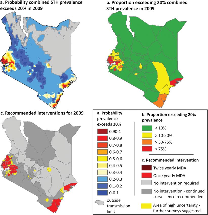
2009). Importantly, the model can then be used to gen- example of such an approach applied to STH infec-
erate a distribution of possible values (i.e. a posterior tions, taken from Pullan et al. (2011a), is shown in
probability distribution) for infection indicators at Fig. 3.
Downloaded from https://www.cambridge.org/core. IP address: 46.4.80.155, on 30 Dec 2020 at 18:15:31, subject to the Cambridge Core terms of use, available at https://www.cambridge.org/core/terms
. https://doi.org/10.1017/S0031182012000698Rachel L. Pullan and others 1874
Fig. 3. An example of the practical applications of a model-based geostatistical (MBG) predictive mapping of soil-
transmitted helminths (STH). (a) Bayesian space-time geostatistical models were developed for each STH species using
survey data from 1980–2009, and were used to interpolate the probability that combined infection prevalence exceeded
the 20% level defined by the World Health Organisation as a mass drug administration (MDA) threshold in 2009. (b)
Population census data were overlaid with the probability models to estimate the proportion of the population at risk
(i.e. >50% probability of exceeding 20% prevalence threshold) and requiring treatment in 2009 for each district.
Recommended intervention districts (c) are defined as: once yearly mass drug administration (MDA), at least 33% of the
district exceeds 20% prevalence threshold, and twice yearly MDA, at least 33% of the district exceeds a 50% prevalence
threshold. Continued surveillance is recommended for districts where historically >75% of the district exceeded the 20%
prevalence based on predictions for 1999, and areas of high uncertainty are those where we can only be 50–65% certain
that prevalence is lower than 20%. Adapted from Pullan et al. 2011.
Although the most common applications of MBG better captured using a negative binomial or zero-
typically use a binomial/logistic regression model inflated Poisson distribution. Alexander et al. (2000)
(i.e. modelling the prevalence/presence of infection), used a negative binomial MBG to model effectively
generalised linear models can handle a variety of data individual Wuchereria bancrofti parasite count data
types. For example, density/intensity of infection can from communities in Papau New Guinea (Alexander
provide a more informative indicator of disease et al. 2000), whilst Brooker et al. (2006) adapted this
burden than simple presence of infection for many model to investigate the small-scale spatial hetero-
parasites. Such data are usually over-dispersed and so geneity in STH and schistosome infections in rural
Downloaded from https://www.cambridge.org/core. IP address: 46.4.80.155, on 30 Dec 2020 at 18:15:31, subject to the Cambridge Core terms of use, available at https://www.cambridge.org/core/terms
. https://doi.org/10.1017/S0031182012000698Spatial parasite ecology and epidemiology 1875
and urban environments in Brazil. Spatial negative contemporary distribution of infection as well as
binomial and zero-inflated Poisson models of faecal changing risks since the launch of large-scale control.
egg count data have also been developed for Spatially explicit approaches can also help better
S. mansoni, S. haematobium and hookworm at com- capture environmental contexts when investigating
munity and country levels (Vounatsou et al. 2009; co-occurrence of parasite species. For example,
Pullan et al. 2010; Soares Magalhães et al. 2011b) and studies have used MBG approaches to investigate
for S. mansoni at regional levels (Clements et al. the geographical distribution of multiple species
2006b). In addition, multinomial models have been infection with helminths and malaria at differing spa-
built to stratify areas on the basis of prevalence of tial scales (Raso et al. 2006b; Brooker and Clements,
high- and low-intensity S. haematobium infections 2009; Pullan et al. 2011b; Soares Magalhaes et al.
in West Africa (Clements et al. 2009b), and to model 2011b; Brooker et al. 2012), facilitating more detailed
the distribution of malaria-helminth co-infections investigation of associations between species. Lastly,
at country (Raso et al. 2006b) and regional levels MBG models have been adapted to better capture
(Brooker and Clements, 2009). Finally, a Bayesian complex, non-linear relationships with covariates
framework allows the inclusion of multiple imputa- thus providing a deeper understanding of the deter-
tion steps. For example, the Malaria Atlas Project has minants of infection. For example, authors have
incorporated a Bayesian model to predict malaria used methods such as penalised spline regression
incidence as a function of parasite prevalence directly (Crainiceanu et al. 2005; Gosoniu et al. 2009; Soares
(Patil et al. 2009) within the geostatistical framework Magalhaes et al. 2011a).
used to model infection prevalence (Hay et al. 2010). Despite their utility, considerable caution must
Data used for mapping parasitic diseases typically be used when building and interpreting complex
originate from a range of sources using various MBG models. For example, careful consideration of
diagnostics, age groups and sampling methods. A appropriate model specifications and priors are essen-
Bayesian inference approach can be adapted to ac- tial to prevent invalid or inefficient inferences. Sys-
count for these additional sources of uncertainty. For tematic changes in diagnostic or sampling methods
example a number of approaches have been used to over time or space can also be misinterpreted as
adjust for combining data from different age groups, genuine change in disease status. Most MBG models
ranging from the inclusion of fixed regression reported in the literature also assume that spatial
coefficients and random alignment factors (Pullan autocorrelation does not vary with location (so-called
et al. 2011a; Schur et al. 2011c) to the incorporation stationary models). Whilst such an assumption may
of mathematical age-standardisation algorithms (Hay be valid across small scales, this may not be true when
et al. 2009; Gething et al. 2011). Diagnostic tests for a considering spatial processes over large geographical
large range of parasites typically have poor sensitivity areas where variation in geography, control, vectors
and specificity, at least in part due to significant day- and even parasite strains can cause spatial variation in
to-day and intra-specimen variation (Utzinger et al. autocorrelation. To tackle this problem, a number of
2001; Booth et al. 2003; Engels and Savioli, 2006; approaches have been developed (Gemperli, 2003;
Farnert, 2008; Leonardo et al. 2008; Tarafder et al. Kim et al. 2005; Raso et al. 2006a, Beck-Worner et al.
2010). In response, in addition to simply adjusting 2007; Gosoniu et al. 2009) although application
for the type of diagnostic method used (Pullan et al. at large spatial scales is still hindered by practical and
2011a), authors have explored bivariate outcome computational constraints. To our knowledge, few
spatial models that allow for calibration of spatially groups have yet to tackle the issue of geographical
correlated data series (Crainiceanu et al. 2008), and anisotropy in parasite epidemiological analyses,
models that include outcomes as random variables although direction is likely to play an important
with ‘informative’ priors defined by observed diag- role in observations of spatial dependency for focally
nostic uncertainties (Wang et al. 2008). transmitted infections such as schistosomiasis and
Another recent extension includes adding a tem- trypanasomiasis (Vounatsou et al. 2009). Stein (2005)
poral dimension. For example, temporal effects have however has proposed a geographically anisotropic
been handled as random coefficients when modelling version of the space-time covariance matrix used
STH prevalence across Kenya (Pullan et al. 2011a) spatio-temporal MBG, that has since been adapted
and malaria across Vietnam (Manh et al. 2010), by Gething et al. (2011) to model the global
explicitly allowing dependency between observations distribution of malaria (Stein, 2005; Gething et al.
within years. This approach has been extended for 2011).
mapping malaria at global scales using a sophisticated Due to the computational burden required to
two-dimensional space-time random coefficient (Hay generate predictions at each individual prediction
et al. 2010), thus simultaneously modelling corre- location, most applications of MBG models tend to
lation between data points in both space and time. be via a ‘per prediction point’ approach, yielding
Such models can provide more accurate predictions marginal prediction intervals that realistically capture
when data are distributed through time as well as appropriate measures of ‘local’ uncertainty. How-
space, providing a better understanding of both the ever, failing to account for spatial or temporal
Downloaded from https://www.cambridge.org/core. IP address: 46.4.80.155, on 30 Dec 2020 at 18:15:31, subject to the Cambridge Core terms of use, available at https://www.cambridge.org/core/terms
. https://doi.org/10.1017/S0031182012000698Rachel L. Pullan and others 1876
Fig. 4. Contrasting predictions of the distribution of Schistosomiasis haematobium generated using similarly robust
MBG regression models, but different data. Model 1: Predicted prevalence of S. haematobium among individuals aged
420 years during the period of 2000–2009, based on survey data from 16 West African countries. Model 2: Predicted
prevalence of S. haematobium infection in boys aged 10–15 years in Burkina Faso, Mali and Ghana in 2004–2006. Inset
maps show the location of survey data used in each model. Although overall trends are similar, these models show
considerable differences in within country distributions, particularly in northern Burkina Faso, central Mali and much
of Ghana. Figures are adapted from Schur et al. 2011 and Soares et al. 2011.
correlation between prediction locations can lead to et al. 2011a; Soares Magalhaes et al. 2011a). This
gross underestimation of uncertainty when aggregat- point is clearly illustrated in Fig. 4. Similar differ-
ing prediction estimates across regions, for example ences are seen for different maps of S. mansoni in East
when producing country-level credible intervals Africa (Clements et al. 2010; Schur et al. 2011b).
(Goovaerts, 2001). A solution is to use joint or simul- Such differences can have important implications for
taneous simulation, which recreates appropriate the planning of control activities and estimations
spatial and temporal correlation in the predictive of populations at risk, and more generally highlight
surface (Goovaerts, 2001), but which can be pro- difficulties in interpreting models from highly
hibitively intensive computationally, especially over spatially heterogeneous data, no matter how sophis-
large areas. Recently however, Gething et al. (2010) ticated the underlying model.
proposed an approximate algorithm for joint simu-
lation, which they applied to a global scale MBG pre-
dictive model for malaria. Importantly, this approach
Quantifying spatial dependency in order to undertake
ensured that aggregated estimates of national and re-
spatial sampling
gional burdens taken from continuous disease maps
still maintained appropriate credible intervals. Data available to the disease mapping community
Final predictive surfaces are also very dependent have usually been collected for other purposes, such
upon available data, a problem which becomes more as to investigate a specific research question or to
pronounced as spatial heterogeneity increases. For determine national or sub-national prevalence esti-
example, a comparison of predictive risk maps of mates, using traditional, probability-based sampling
S. haematobium in West Africa generated using simi- methods (Levy and Lemeshow, 2008). Such design-
larly robust MBG approaches but different datasets based sampling forms the basis of most prevalence
gives rise to maps which, whilst having similar surveys for parasitic infections, including those for
regional trends, exhibit large differences in within- Plasmodium infection (Roll Back Malaria Monitoring
country distributions (Clements et al. 2009b; Schur and Evaluation Reference Group, 2005), STHs
Downloaded from https://www.cambridge.org/core. IP address: 46.4.80.155, on 30 Dec 2020 at 18:15:31, subject to the Cambridge Core terms of use, available at https://www.cambridge.org/core/terms
. https://doi.org/10.1017/S0031182012000698Spatial parasite ecology and epidemiology 1877
Fig. 5. (a) Illustrative example of the lattice plus close pairs design using a grid size of 50 km to select schools for
surveys of S. mansoni in Oromia Regional State, Ethiopia. Dark points refer to selected schools and gray points to
unselected schools. (b) A close-up of a region (black box in a) showing the locations of some of the clusters of closely
located schools. Adapted from Sturrock et al. (2011).
(World Health Organization, 2006) and schisto- between any point in an area to its nearest survey
somiasis (World Health Organization, 2006). We site, such that an uniform distribution of sites over
now know from other disciplines, such as geology and areas of any shape or size is obtained.
environmental sciences, that where MBG mapping The selection of survey sites can also be informed
is the eventual goal, such design-based sampling by an understanding of the spatial structure of the
may be suboptimal and instead purposive (non- outcome to be surveyed. For example, if the spatial
probability-based) sampling is generally more effici- structure of the data is known (based on a semi-
ent (Brus and de Gruijter, 1997; de Gruijter et al. variogram), it is possible to estimate the kriging
2006). Such purposive sampling does not involve a variance of any configuration of survey sites a priori.
random selection of sites, rather sites are selected This feature makes it possible to optimise the
based on their location or characteristics (i.e. selected locations of surveys for spatial prediction before
to represent a particular altitude or ecological zone). data are gathered (Van Groenigen et al. 1999; Brus
The majority of early applications of spatial sampling et al. 2006). Where the autocorrelation structure
came from ecological or soil science, but there are is unknown or uncertain, pilot surveys can be con-
now an increasing number of applications in infec- ducted to quantify the spatial characteristics, which
tious disease epidemiology, which we review here. can then be used to optimize secondary data collec-
Recent surveys of schistosome infection have tion (Stein and Ettema, 2003). Alternatively, Diggle
adopted a stratified cluster random sampling design and Lophaven (2006) propose the use of a lattice plus
in order to obtain a spatially representative sample for close pairs design which is formed of a regular grid of
subsequent risk mapping (Clements et al. 2006a, b, points with some additional sites clustered around a
2009b). A qualitative approach to selecting survey selected number of grid sites. Fig. 5 provides an
locations was adopted in a recent nationwide school illustration of the lattice plus close pairs design for the
survey of Plasmodium infection in Kenya (Gitonga selection of schools in a survey of S. mansoni in
et al. 2010), whereby the selection of schools in Ethiopia. First, a grid of a predefined size is placed
each district was made with a non-probability-based over the survey region and those schools lying closest
method to ensure a representative spatial spread of to the interstices of the grid are selected. Second, at
points. Furthermore, sites were over-sampled in some of these schools, the five closest neighbouring
sparsely populated districts to allow efficient spatial schools are selected. This stepwise selection ensures
interpolation in these areas. An alternative approach both a good spread of sample sites which are efficient
is spatial coverage sampling, whereby survey sites for spatial interpolation and some closely located sites
are selected to ensure maximum coverage over a which are important for quantifying the spatial struc-
given survey region, accounting for its shape and ture of the outcome. Recent work by Sturrock et al.
previously collected data (de Gruijter et al. 2006). (2011) demonstrates that use of a lattice plus close
Van Groenigen et al. (2000) have, for example, used pairs design followed by kriging provided a more
an iterative process to determine the configuration of cost-effective approach to identify schools with high
sites for soil sampling that minimises the distance prevalence of S. mansoni compared to sampling a
Downloaded from https://www.cambridge.org/core. IP address: 46.4.80.155, on 30 Dec 2020 at 18:15:31, subject to the Cambridge Core terms of use, available at https://www.cambridge.org/core/terms
. https://doi.org/10.1017/S0031182012000698Rachel L. Pullan and others 1878
small number of children in every school using lot may be difficult to obtain sufficient point-level data to
quality assurance sampling (LQAS). This work model spatial variation in infection risk effectively,
shows that, whilst LQAS performed better than due to financial or practical constraints. In such
spatial sampling in identifying schools with a high instances, it may be more appropriate to make best
prevalence, its cost-effectiveness in identifying such use of spatially discrete data using hierarchical
schools was lower. techniques. Whilst the primary focus of authors de-
Researchers have recently begun to investigate veloping such techniques has often been in improv-
optimal survey designs that also incorporate covariate ing demographic and sociological data (Hentschel
information (such as environmental and climatic et al. 2000), or in modelling the distribution of
factors) when collecting data for mapping based on non-communicable disease (Jackson et al. 2008b;
MBG techniques. Unlike optimizing sampling for Yiannakoulias et al. 2009; Danaei et al. 2011), many
spatial interpolation alone, optimizing sampling for of these methods are also applicable to parasitological
mapping using MBG with covariates requires a and related data only available at an area level, for
spread of points in so-called feature space (i.e. across example the number of malaria cases or intervention
the full range of included covariates) as well as across population coverage. In the next section we discuss
geographic space. To find a balance between these some of these applications, drawing on examples
differing requirements, Hengl et al. (2003) propose from beyond the infectious disease literature where
an ‘equal-range strategy’ which ensures that equal necessary.
numbers of sites are randomly selected in areas
stratified by relevant covariates. By repeating this
Discrete spatial variation: modelling discrete
process multiple times, the sampling design with the
outcome data
most comprehensive spatial coverage can be chosen.
Researchers have also used universal kriging variance A major objective when modelling discrete disease
to optimize surveys for soil, groundwater dynamics data is obtaining statistically precise local estimates of
and radioactive releases (Heuvelink et al. 2006; Brus the outcome of interest, whilst maintaining fine-scale
and Heuvelink, 2007; Melles et al. 2011). By finding geographic resolution. This can be a considerable
the configuration of sites that minimises the universal challenge when outcomes are rare or sample sizes are
kriging variance, a balance is struck between opti- small, as small stochastic differences between areas in
mizing sampling across feature and geographic space. the number of cases can result in large apparent
An appeal of this approach is that any number of differences in the distribution of the outcome. By
covariates can be included, making it theoretically smoothing high-resolution variability, model-based
plausible to optimise surveys for multiple species approaches can compromise between (overly) un-
with differing environmental niches. Such stratified certain within-area estimates and (overly) simplified
sampling designs do however come with an impor- aggregated higher level estimates, thus stabilising
tant caveat: over-sampling in areas with particular estimation from areas with small populations or
characteristics (such as known higher infection sample sizes (Goldstein, 1995). Such approaches,
prevalence) does risk invalidating standard geostatis- based upon the use of generalised linear mixed effect
tical inference, as the implicit assumption of this models, form the basis of small area estimation, with
approach is of non-preferential sampling. Never- wide application in the analysis of health and social
theless, given the recent increase in advocacy for survey data (Ghosh and Rao, 1994; Ghosh et al. 1998;
integrated control of multiple parasite species, an Richardson and Best, 2003; Asiimwea et al. 2011).
investigation into optimal survey methods that con- They are inherently non-spatial, borrowing infor-
sider both environmental correlates and spatial mation across all areas without considering spatial
dependency for multiple species is clearly warranted. location, and smoothing to the global mean. How-
ever, they can easily be extended to include additional
model complexity such as spatial dependence using
D I S C R E T E S P A T I A L VA R I A T I O N :
discrete spatial smoothing models based on proxi-
UNDERSTANDING SPATIAL NEIGHBOURHOOD
mity. Such models, which assume positive spatial
STRUCTURE
correlation between observations, essentially borrow
The methods described above depend on two major more information from close neighbours than
assumptions: that the underlying spatial process is those further away, and so smooth local rates to-
continuous and that sufficiently detailed point-level wards local, neighbouring values (Waller and Carlin,
data are available to capture this process. Certain data 2010).
may only be available at a small-area level (for One of the first examples of spatial discrete model-
example, routine health surveillance data, access to ling is provided by Clayton and Kaldor (1987), who
water and sanitation, quality of local health services), developed a Poisson regression model with area-
and as such autocorrelation may only be apparent be- specific random intercepts defined using a conditional
tween immediate neighbours (i.e. based upon proxi- autoregressive (CAR) structure to model standardised
mity rather than actual location). Alternatively, it mortality ratios (in this case, cancer rates). By this
Downloaded from https://www.cambridge.org/core. IP address: 46.4.80.155, on 30 Dec 2020 at 18:15:31, subject to the Cambridge Core terms of use, available at https://www.cambridge.org/core/terms
. https://doi.org/10.1017/S0031182012000698Spatial parasite ecology and epidemiology 1879
approach, the area-specific random effect is generated across the study area, and in all directions. This issue
using a simple adjacency weights matrix, such that was recently tackled in part by Reich and colleagues
for each observation the associated random parameter (2007), who developed a 2NRCAR (CAR prior with
has a weighted mean given by a simple average of two neighbour relations) model that is able to accom-
its defined neighbours and a conditional variance modate two difference classes of neighbour relations
inversely proportion to the number of neighbours. (e.g. east-west and north-south) (Reich et al. 2007),
This model has since been extended to a fully although to our knowledge this has yet to be applied
Bayesian formulation (Besag et al. 1991) and can be in an epidemiological context. A third issue concerns
readily implemented in standard Bayesian inference the often arbitrarily defined units of representation
software. Via this flexible inference platform, spatial available for geographical analysis. This is known as
CAR models can be structured to allow autocorrela- the modifiable areal unit problem, by which for any
tion between adjacent neighbours only, or to allow specified number of spatial units, there are many
spatial smoothing to extend to more distant neigh- ways of defining the boundaries of these units, which
bours (Wakefield, 2004; MacNab, 2010), and can be can produce very different results (Openshaw and
extended to allow for: estimation of spatially varying Taylor, 1979). For example, spatial anomalies may go
covariates; prediction of missing data; inclusion undetected if the scale of the underlying spatial
of both spatial and non-spatial dependency; and heterogeneity is smaller than the area unit available.
inclusion of spatio-temporal and multivariate out- Although this cannot be completely overcome, care-
come covariance structures (Mollie, 1996; Waller and ful consideration of CAR and MM models does allow
Carlin, 2010). smoothing between units, thus blurring the concept
A similar but less commonly used class of models of a discrete unit of analysis.
are the spatial multiple membership (MM) models,
which examine to what extent a latent spatially distri-
buted variable can explain the outcomes of interest
Discrete spatial variation: combining point and
(Breslow and Clayton, 1993; Goldstein, 1995;
area level data
Langford et al. 1999; Browne et al. 2001). In contrast
to CAR models, the spatial dependence here is In many instances, disease data may be available at a
modelled through the multiple membership relation- point level (e.g. survey or sentinel site data), although
ship, with an independent area-level random effect. covariate information may be available only at an area
CAR and MM approaches have most widely been level. For example, although recognised as important
applied to modelling rates of rare non-communicable factors influencing the distribution of parasitic dis-
diseases, such as cancer and heart disease (Lawson, eases at varying spatial scales, data on factors such as
2006), usually in a developed country setting where water supply, sanitation and hygiene (WASH), own-
comprehensive disease registry data are available. ership and use of bednets, coverage of interventions
However in tropical epidemiology, analyses of such as mass drug administration, and poverty and
routinely collected surveillance data have used spatial deprivation indicators may only be available at dis-
CAR and MM models on varying scales to investigate trict and regional levels (Esrey et al. 1991; Kazembe
incidence of malaria in Zimbabwe, South Africa and et al. 2007; Soares Magalhaes et al. 2011a). Alterna-
China (Kleinschmidt et al. 2002; Mabaso et al. 2006; tively, disease information may only be available
Clements et al. 2009c) and dengue in Rio de Janeiro, aggregated at area-levels for rare outcomes, although
Brazil (Teixeria and Cruz, 2011) in addition to individual-level survey data describing the distri-
assisting in the geographical targeting of schisto- bution of explanatory factors may be readily avail-
somiasis control in Tanzania using collated ques- able. Despite the aggregated nature of such data,
tionnaire data (Clements et al. 2008b). careful analysis can provide information about the
There are a number of substantial methodological relationships between area-level risks and point-level
challenges when modelling spatially discrete data. outcomes. This process is known as ecological infer-
The first of these concerns assumptions made regard- ence (Richardson and Monfort, 2000; Jackson et al.
ing the underlying spatial process. Discrete spatial 2006, 2008a), and can be valuable when the effect of a
variation models consider the location of data points variable is believed to operate through its area-level
in terms of proximity only, rather than as literal average (sometimes termed a contextual effect) (Begg
positions, and as such the model is valid only for and Parides, 2003). For instance, control policies for
included data; validity is not necessarily preserved if many parasitic infections implemented at the district
further locations are added to the data (Diggle, 2004). level have been shown to benefit indirectly those
For this reason, these models are not appropriate for individuals who have not participated. Helminth in-
spatial prediction in new locations (interpolation). As fection prevalence in non-compliant or non-targeted
for methods quantifying continuous spatial depen- individuals, for example, is typically seen to reduce
dency, discrete spatial approaches also model global after the administration of community or school-
spatial structure and thus assume that the degree of based mass chemotherapy (Bundy et al. 1990; Chan
correlation between neighbouring units is consistent et al. 1997; Vanamail et al. 2005; Mathieu et al. 2006;
Downloaded from https://www.cambridge.org/core. IP address: 46.4.80.155, on 30 Dec 2020 at 18:15:31, subject to the Cambridge Core terms of use, available at https://www.cambridge.org/core/terms
. https://doi.org/10.1017/S0031182012000698Rachel L. Pullan and others 1880
El-Setouhy et al. 2007). This is primarily due to a problematic in practice, as obtaining data on the same
reduction in the force of transmission, analogous to population from different sources may lead to con-
the ‘herd immunity effect’ seen for vaccines. How- siderable inconsistencies, such as differences in
ever, in many instances area-level exposure-response variable definition and reporting, timing, and even
relationships may not accurately reflect associations geographical boundaries between levels, which may
at the community or household level, a process in turn lead to unreliable conclusions (Jackson et al.
known as the ecological fallacy or ecological bias 2008a).
(Morgenstern, 2008). For example, an individual-
level association between individual socio-economic
SPATIAL POINT PROCESSES: INVESTIGATING
indicators and regional rates of disease does not
SPATIAL CLUSTERING
necessarily imply an effect of socio-economic status
on individual infection status. It can equally be The global spatial statistics described above provide
caused by other confounding factors. an important set of epidemiological tools to inform
The magnitude of ecological bias depends upon whether spatial heterogeneity is present throughout
the degree of within-area variability in exposures and spatially sampled measurement data. This in turn
confounders – if there is no variability, all individuals informs optimal model building and can be used to
will experience the same degree of exposure, and so conduct spatial interpolation and prediction. These
there will be no ecological bias (Wakefield and Lyons, methods cannot be used to delineate explicitly the
2010). The only way to truly overcome the problem locations of individual clusters and typically make the
of ecological bias therefore is to supplement aggregate assumption that the magnitude and scale of cluster-
data with samples of data at the individual level, ing is equal throughout the study region. Identifying
which on their own may be too sparse to accurately the propensity for spatial clustering to occur, or the
capture geographic variation but can provide an physical locations of individual clusters, is vital for
indication of intra-unit variation. Several theoretical both identifying areas with higher than expected
methods have been proposed to do this, which can be underlying risk and detecting outbreaks, as well as
used to address bias and separate individual and determining the optimal spatial location and scale of
contextual effects when either the outcome or the interventions. It is also important to emphasise that,
exposure measure is available at an ecological level whilst identifying the presence of spatial clusters may
(Prentice and Sheppard, 1995; Steel and Holt, 1996; be useful, it is perhaps more important epidemio-
Lasserre et al. 2000; Best et al. 2001; Wakefield and logically also to gain a deeper understanding of the
Salway, 2001; Glynn et al. 2008). The so-called determinants of this clustering (Rothman, 1990;
aggregate data method, for example, estimates Alexander and Boyle, 2001).
individual-level exposure effects by regressing popu- Point process statistics aims to analyse the explicit
lation-based disease rates on covariate data from location of events distributed in space under an
survey samples in each population group (Prentice assumption that the spatial pattern is random (i.e. the
and Sheppard, 1995). An alternative approach, locations and numbers of points are not fixed). In
termed hierarchical related regression, assumes a dis- parasite epidemiology and ecology, such data typi-
tribution for within-area variability in exposure, and cally present either as point locations within a given
fits the implied model to aggregate data combined study area (for example, residence of incident cases or
with small samples of individual-level exposure and location of vector breeding sites) or as counts of cases
outcome data (Jackson et al. 2006, 2008a). from administrative districts partitioning the study
Both of these approaches however are not inher- area (Waller, 2010). Point process approaches typi-
ently spatial, although the generalised linear model cally play two distinct roles in the analysis of such
frameworks upon which they are based can in theory data. First, they can be used to investigate the general
be adapted to include multiple levels of aggregation tendency of points to exist near points, providing
and spatial dependency between baseline risks. For a global measure of clustering averaged across the
example, spatial CAR models have been combined observed point locations. For example, we may be
with aggregate data methods to account better for interested in whether summary global measures of
exposure effect when modelling spatially hetero- clustering for disease cases differ significantly from
geneous breast cancer rates (Guthrie et al. 2002), those for the general at-risk population, and thus
and with hierarchical related regression when inves- whether there is an overall tendency for cases to occur
tigating sensitivity of environmental exposure and near other cases rather than to occur homogeneously
childhood leukaemia data to ecological bias (Best among the population at risk. Secondly, they can be
et al. 2001). These approaches have yet to be applied used to delineate explicitly the locations of individual
within an infectious disease context, but they do have clusters, or anomalous collections of points. Such
great potential for application in spatial parasite clusters might be assumed to occur anywhere within
epidemiology, for example, to improve evaluation the study area, or may be focused, centred around pre-
of intervention programmes using implementation- defined foci of putatively increased risk (e.g. vector or
level, sentinel site and cluster-level data. This may be intermediate host breeding sites) (Besag and Newell,
Downloaded from https://www.cambridge.org/core. IP address: 46.4.80.155, on 30 Dec 2020 at 18:15:31, subject to the Cambridge Core terms of use, available at https://www.cambridge.org/core/terms
. https://doi.org/10.1017/S0031182012000698Spatial parasite ecology and epidemiology 1881
1991). In both scenarios, analysis strategies usually statistical framework for investigating spatial hetero-
build upon ideas of testing the hypothesis of com- geneity, whilst adjusting for spatially varying risk
plete spatial randomness (CSR), such as the realis- factors. The more fundamental of these models are
ation of a homogeneous Poisson process (Isham, based upon the non-homogeneous Poisson process,
2010). In epidemiology, this is often complicated by which assumes a lack of interaction between points
the heterogeneous distribution of the at-risk popu- (i.e. complete spatial randomness) but still allows
lation, with the null model of interest no longer being point intensity to vary over space. This assumption of
CSR, but one of spatially constant risk, and thus independence between points may be appropriate if
knowledge of the underlying distribution of the all spatial variation can be explained by observed or
population at-risk, or of appropriate non-infected unobserved risk factors, such as climate, topography
controls, is essential (Waller, 2010). and inherited genetic risk, which are themselves
There is a rich body of literature addressing various spatially correlated, an assumption often fitting for
approaches for spatial point processes, although their non-infectious diseases (Diggle, 2001). For infec-
existing application to the ecology and epidemiology tious diseases however, stochastic spatial dependence
of parasitic diseases has to date been somewhat may still remain between points even after accounting
limited in scope. This is partly due to the fact that for covariates. For example, foci of parasite trans-
model fitting is not straightforward and often com- mission can perpetuate and amplify spatial hetero-
putationally complex. In addition, many approaches geneity, with heavily infected individuals shedding
have been derived from a rather mathematical pers- large numbers of parasites into the environment,
pective and are not necessarily appropriate in an increasing risk for those living in close proximity.
ecological or epidemiological context. We do not This can be modelled by hierarchical processes
therefore provide a comprehensive review of all avail- derived from the above non-homogeneous Poisson
able methods here, but instead compare and illustrate process, including Poisson cluster and Cox processes.
some of the most popular contemporary approaches These flexible models are ‘doubly stochastic’ in that
for detecting clustering and clusters in parasite epi- they also include a random intensity function, which
demiology. More complete general reviews of may be taken to be any random spatial process. As
methods and applications appear elsewhere (Diggle, such, they are very effective for describing residual
2003; Waller and Gotway, 2004; Gelfand et al. 2010). positive association between points. For example,
sophisticated log-Gaussian Cox process models,
which assume a Gaussian random field for the
logarithm of the density function (analogous to
Detecting global clustering in point pattern data
the Gaussian geostatistical models detailed above),
Investigations of global clustering usually start by have been applied to investigations of tick-borne
testing benchmark hypotheses regarding the under- encephalitis in the Czech Republic (Benes et al.
lying process – i.e. is a point or case equally likely to 2011), and spatio-temporal surveillance of non-
occur at any location? Such hypothesis testing ap- specific gastroenteric disease in the UK (Diggle
proaches include Ripley’s K function (Ripley, 1976) et al. 2005). However, despite increased application
and the related L function (Besag, 1977), which pro- in other areas of spatial epidemiology (Lawson, 2006)
vide a measure of the (scaled) number of additional to our knowledge we have yet to see these potentially
events expected within distance h of a randomly exciting methods being applied to parasite ecology.
selected point. Plotting K as a function of h can thus
be used to describe characteristics of the point process
at many different spatial scales. More recent appli-
Detecting local clusters in point pattern data
cation of these methods to infectious disease epi-
demiology includes investigation of urban dynamics Although restricted to hypothesis testing, methods
of dengue epidemics in the Brazilian city of Belo for detecting local clusters in point pattern data are
Horizone (Almeida et al. 2008), identification of perhaps the most popular point process statistical
epidemic hotspots for malaria in the Kenyan western techniques currently used by parasite epidemiolo-
highlands (Wanjala et al. 2011), and investigation of gists, with a variety of methods available for ex-
spatial clustering of households with seropositive ploring and identifying clusters in both point and
children during evaluation of targeted screening aggregated data (for an excellent review see Pfeiffer
strategies to detect Trypanasoma cruzi infection in et al. 2008). The more popular approaches involve
Peru (Levy et al. 2007). spatial scan statistics, the most developed of these
In recent years, summary test-based measures being Kulldorff’s spatial scan statistic (Kulldorff and
for spatial point processes have been joined by Nagarwalla, 1995). This method constructs a series
model-based approaches, using both frequentist and of circles of increasing size around each data location
Bayesian inference platforms. As with models of con- and compares the level of risk within each circle to
tinuous and discrete spatial variation, spatial point that outside using a likelihood ratio test. A compu-
process models provide an objective and efficient tationally convenient Monte Carlo simulation is then
Downloaded from https://www.cambridge.org/core. IP address: 46.4.80.155, on 30 Dec 2020 at 18:15:31, subject to the Cambridge Core terms of use, available at https://www.cambridge.org/core/terms
. https://doi.org/10.1017/S0031182012000698You can also read