The Physics of Financial Networks
←
→
Page content transcription
If your browser does not render page correctly, please read the page content below
The Physics of Financial Networks
                                                 Marco Bardoscia1,2,* , Paolo Barucca2 , Stefano Battiston3,4 , Fabio Caccioli2,5,6 , Giulio
                                                 Cimini7,8,9 , Diego Garlaschelli8,10 , Fabio Saracco8 , Tiziano Squartini8 , and Guido
                                                 Caldarelli11,12,9,13,B
                                                 1 Bank of England, London, UK
                                                 2 University College London, Department of Computer Science, London, UK
                                                 3 University of Zurich, Department of Banking and Finance, Zurich, Switzerland
                                                 4 University of Venice “Ca’ Foscari”, Department of Economics, Venice, Italy
arXiv:2103.05623v1 [physics.soc-ph] 9 Mar 2021

                                                 5 Systemic Risk Centre, London School of Economics and Political Sciences, London, UK
                                                 6 London Mathematical Laboratory, London, UK
                                                 7 University of Rome “Tor Vergata”, Department of Physics and INFN, Rome, Italy
                                                 8 IMT School for Advanced Studies, Networks Unit, Lucca, Italy
                                                 9 Consiglio Nazionale delle Ricerche, Institute of Complex Systems, Rome, Italy
                                                 10 Lorentz Institute for Theoretical Physics, University of Leiden, Leiden, The Netherlands
                                                 11 Department of Molecular Science and Nanosystems, University of Venice “Ca’ Foscari”, Venice, Italy
                                                 12 European Centre of Living Technologies, University of Venice “Ca’ Foscari”, Venice, Italy
                                                 13 London Institute for Mathematical Sciences, London, UK
                                                 * Any views expressed are solely those of the author(s) and so cannot be taken to represent those of the Bank of

                                                 England or to state Bank of England policy.
                                                 B Guido.Caldarelli@unive.it

                                                 ABSTRACT

                                                 The field of Financial Networks is a paramount example of the novel applications of Statistical Physics that have made possible
                                                 by the present data revolution. As the total value of the global financial market has vastly outgrown the value of the real economy,
                                                 financial institutions on this planet have created a web of interactions whose size and topology calls for a quantitative analysis
                                                 by means of Complex Networks. Financial Networks are not only a playground for the use of basic tools of statistical physics
                                                 as ensemble representation and entropy maximization; rather, their particular dynamics and evolution triggered theoretical
                                                 advancements as the definition of DebtRank to measure the impact and diffusion of shocks in the whole systems. In this review
                                                 we present the state of the art in this field, starting from the different definitions of financial networks (based either on loans,
                                                 on assets ownership, on contracts involving several parties – such as credit default swaps, to multiplex representation when
                                                 firms are introduced in the game and a link with real economy is drawn) and then discussing the various dynamics of financial
                                                 contagion as well as applications in financial network inference and validation. We believe that this analysis is particularly
                                                 timely since financial stability as well as recent innovations in climate finance, once properly analysed and understood in terms
                                                 of complex network theory, can play a pivotal role in the transformation of our society towards a more sustainable world.

                                                 1 Introduction
                                                 Statistical physics provides a mathematical description of the relation between microscopic and macroscopic properties of
                                                 physical systems composed by many parts. For this reason, in the last decades, statistical physics has emerged as a legitimate
                                                 approach to investigate such a relation in social and economic systems1–5 . In particular, the study of complex networks and
                                                 their applications to economics and finance has become a playground for the discipline6–12 . Especially in the field of financial
                                                 networks the application of physics to social systems has been greatly successful in terms of results and impact13–18 . Aim of
                                                 this review is to present the main research questions and results, and the future avenues of research in this field. It is widely
                                                 recognized today that modelling the financial system as a network is a precondition to understand and manage a wide range
                                                 of phenomena that are not just relevant to finance professionals or scholars, but also to researchers in many other disciplines,
                                                 ordinary citizens, public agencies and governments19, 20 . Indeed, the implications of dysfunctions in the financial system include:
                                                 ordinary citizens losing jobs and savings as in the 2009 financial crisis; public budgets going into deficit (thus shrinking also
                                                 funding for scientific research) as in the 2012 sovereign crisis; excessive investments flowing into carbon-intensive economic
                                                 activities, thus jeopardising the achievement of the climate mitigation objectives of the Paris Agreement.
                                                     The discipline of financial networks has filled an important scientific gap, by showing that many important phenomena in
                                                 the financial system emerge because of the indirect interaction of financial actors. This means, for example, that if the price of a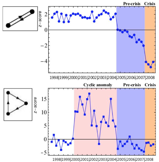
(a)                               (b)

                                                        Liabilities                       Liabilities
                                                                           Assets
                                         Assets
                                                                                           Equity
                                                         Equity
                                                                             x                x

                                                  A                       x   A x   x    x
                                             λ=     = 2                     =  ⋅ = λ = 2
                                                  E                       E E A     A    A

Figure 1. Stylised balance sheet of an investor with leverage λ = 2 (a). Shocks to assets translate into equity shocks amplified
by a factor λ (b).

certain asset plummets, not only those actors who have invested in that asset are affected, but also those who have invested in
the obligations of the former actors. Because of the intricate chains of contracts, and the feedback mechanisms, the resulting
effects can be much larger than the initial shocks. As in other domains of complex systems, the emergence of system-level
instabilities can only be understood from the interplay of the network structure (e.g. closed chains) and key properties of links
and nodes (e.g. about risk propagation and financial leverage)21, 22 . Traditional economic models have described the financial
system either as an aggregate entity or as a collection of actors in isolation, failing to provide an appropriate description of
these mechanisms and their implications for society23 .
    The discipline of financial networks, has been very interdisciplinary from the start, positioned at the frontier of graph theory,
statistical physics of networks, financial economics. The units of observation (e.g. financial actors with their balance sheets
and their contracts) belong by their nature to the domain of economics and finance, as do areas of applications such as the
analysis of corporate influence and systemic risk. Once the initial questions24–26 have been analysed in terms of network theory,
new methods and insights have emerged, in particular in the statistical physics community, that have enriched the initial set of
questions: when does the network amplify or absorb risk? How does the network structure interplay with the feature of the risk
propagation process? How does the network structure and the expectations of the financial actors co-evolve?
    The discipline of financial networks has delivered statistical tools and analytical models to characterise financial risk beyond
the traditional boundaries of economics by accounting for the complexity and the interconnectedness of the financial system.
The key contributions to this endeavour are demonstrated by the adoption of concepts and metrics by practitioners and policy
makers in the financial sector27–29 and by scholars in the economics profession30–32 .

  Box 1: Leverage
  Investors are said to be leveraged when they borrow money to invest. For instance, we use leverage when we get a
  mortgage to buy a house. If we put a capital of £ 40 000 as a downpayment and we borrow £ 160 000 to buy a house
  worth £ 200 000, then our leverage is equal to 5: the value of our assets (the house) divided by our capital. Leverage is
  related to risk, because it amplifies our gains and losses. If the value of the house increases to £ 220 000, we could sell it,
  pay back our debt (let us assume for simplicity there is no interest rate), and we would have gained £ 20 000. We see then
  that an increase of 10% in the value of the house translates into an increase of 50% of our initial capital. The same is
  however true if the house is devalued: a devaluation of 10% would lead to a 50% reduction of our initial capital (from
  £ 40 000 to £ 20 000). More in general, if our leverage is equal to λ , a 1% change in the value of the house translates
  into a λ % change of our capital. The same applies to all leveraged investors. Leverage λ is defined in general for any
  investor or institution as the ratio between assets and equity. In Figure 1 we show the stylized representation of a balance
  sheet of an investor with leverage equal to two. When the assets are devalued by 25% the equity lost is 50%, equal to the
  asset devaluation multiplied by leverage: The higher leverage, the higher the amplification of losses, the higher the risk of
  the investor. So far we have considered an isolated investor, but the concept of leverage as an amplifier of losses can be
  generalized to the context of a network of interconnected balance sheets. For instance, when banks lend money to each
  other, the interbank assets of a bank correspond to the interbank liabilities of other banks. When a bank is under stress, the
  value of the interbank assets associated with its liabilities are devalued, which puts its creditors under stress, and so on.
  It can be shown that the propagation of shocks within the network is governed by a matrix, called matrix of interbank
  leverage, whose leading eigenvalue determines the level of endogenous amplification of exogenous shocks21 .

                                                                                                                               2/23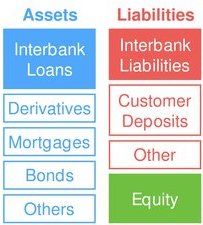
2 Network structure
2.1 The financial system as a network
The financial system consists of financial actors (e.g. institutions such as banks, or pension funds, but also small “fintech”
companies or households), markets (e.g. the stock, or the bond market), contracts (e.g. the ownership in a stock, or a loan
between two banks, or from a bank to a firm, or from a bank to a household), and regulatory bodies (e.g. financial supervisors
and central banks). A network is thus a natural description of the financial system. Nodes represent financial actors and links
may represents contracts or other types of relations (e.g. two actors investing in the same asset). There are processes occurring
on the financial network, where the properties of nodes change but the link remain the same, such as the flow of revenues from
economic activities to the owners of the corresponding securities, or the propagation of losses. Furthermore, in a financial
network the relationships change over time. As a result, a complete description of the financial system requires a temporal
multiplex network, where each layer is associated with a specific type of relationship (e.g. interbank loans of a given maturity).
The emergent macroscopic properties of the network are then important to understand questions of general interest such as the
conditions for having financial stability or a smooth transition to a low-carbon economy. However, the structure of financial
networks evolves also as a result of actors trying to anticipate the future of the network itself in competition with other nodes.
This feedback loop makes the investigation of the emergent properties of financial networks a fascinating scientific challenge
that differs fundamentally from questions pertaining networks in the natural science domains.
In this review we proceed in the following order. We start with the characterization of the structure of static financial
networks, single and multiplex. We then review the most studied processes taking place on financial networks, focusing on
financial contagion, first along bilateral links in unipartite networks, and then through common neighbouring nodes (overlapping
portfolios) on bi-partite networks. Further, we cover the problem of estimating the structure of the financial networks from
partial information. More in general, we review the stream of works on constructing ensembles of financial networks that
satisfy certain properties on average or in distribution.
In order to describe both the structure and the microscopic processes taking place on financial networks, we will have to
introduce some specific notions and jargon. However, we will try to map them in terms of nodes, links and physical analogs in
order to highlight similarities and differences with other related to other areas of physics, such as contact processes33 , diffusion
theory34 , and epidemics35 .
2.2 Single-layer networks
While economic networks comprise several types of relations, such as credit lending or supply of goods and services, the
network of ownership best reflects the relations of power36, 37 among economic and financial actors. Through chains of
ownership, shareholders have a means to influence, intentionally or not, the activities of firms owned directly and indirectly.
Thus, one stream of work has investigated the structure of ownership networks and its implications. Ownership networks
display small world properties24, 38, 39 , scale-free network properties appear in stock markets across countries40, 41 , the global
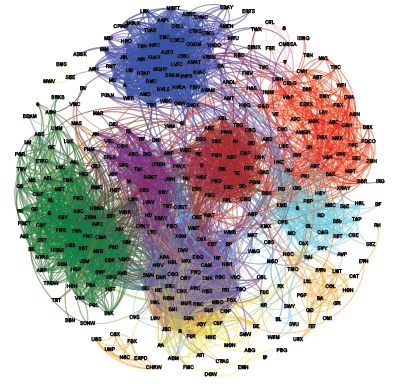
network of ownership has a bow-tie structure with a very concentrated core of financial companies42 – a community structure
that reflects geopolitical blocks43 , while the embedding into geographical space explains several of the network properties44 .
The global ownership network appears to be very resilient in terms of the power structure, even to the dramatic events of the
2008 financial crisis45 .
One stream of work since the early days of the discipline has focused on the structure of the network of credit contract among
financial institutions (hereafter interbank credit network). These networks are the natural and simplest empirical counterpart
for many of the financial contagion models (see Section 3). However, data on these type of relationships is confidential and
available only to or through financial supervisors. In the very recent years, some supervisors have gained access to data that
correspond to daily multiplex, cross boundary networks (e.g. data on derivative contracts collected in Trade Repositories46, 47 ).
However, in the beginning, only static data was available for individual countries, due to boundary issues. Empirical papers
have analysed interbank networks in several countries. The early works on Austria48 and US49 , paved the way to a stream
of works covering e.g. Brazil50, 51 , Belgium52 , Colombia53 , Germany54 , Italy55–58 , Japan59 , Mexico60 , Switzerland61 ,US62, 63 .
Overall, the above works have highlighted in national banking systems the existence of some stylized facts, i.e. statistical
features that are common across the different networks. These financial networks were found to be typically very sparse, with
heavy-tailed degree distributions, high clustering and short average path length, being disassortative.
A specific strand of the literature has focused on characterising the underlying topology of those networks. A few studies
looked for the most appropriate emergent block description of financial networks, whether they feature a subset of tightly-
connected institutions, the core, and a subset of institutions, the periphery, which are loosely connected among each other and
often connected to the core64–68 . Post-crisis, the establishment of central clearing counterparties (CCPs) has meant that many
contracts were rerouted through a single institution (the CCP). The potential benefits and risks of such change in the network
topology have been investigated in69–75 .
3/23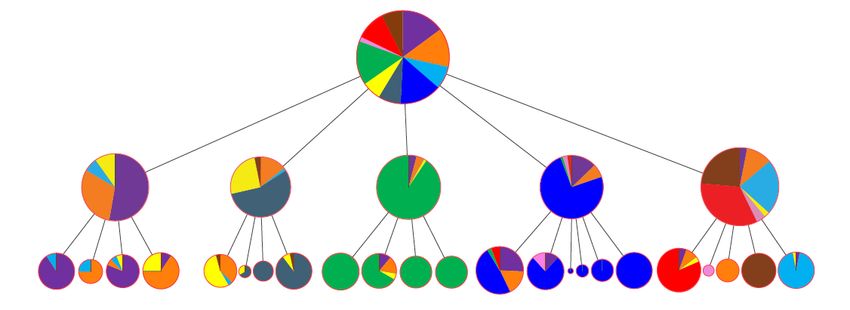
2.3 Multiplex and higher-order networks
The financial networks discussed so far condense all the information about the relationships between a pair of financial
institutions into one (weighted) edge. This is often a useful abstraction, but in realty those relationships are more complex and
this can matter for the propagation of risk. Multiplex networks76, 77 provide a natural framework to describe such relationships
and first empirical studies have shown that different layers are not structurally similar. Examples include: credit and liquidity
exposures in the UK interbank market78 , payments and exposures in the Mexican banking system60 , the Mexican interbank
market79 , the Italian interbank market80 , Colombian financial institutions and market infrastructures81 , the EU derivatives
market28 , the UK interest rate, foreign exchange, and credit derivatives market47 , corporate networks82 . Several works have
focused on financial contagion on multiplex networks, see Section 3.3.
    Another fruitful area of investigation has been the network implied by the derivative market. Due to data availability, most
early studies have focused on credit default swaps (CDSs), derivative contracts in which an institution offers to insure another
institution over the default of a third institution. As such, they are an example of three-body interactions. The existence of
this market should allow institutions to hedge their risks and provide a solid market valuation of the financial risk of different
market players. Nevertheless, CDS markets, as shown in a series of financial networks studies28, 83–85 , can themselves become
a channel of contagion in the possible situation where CDS insurers absorb too much risk upon themselves46 .

2.4 Correlation- and similarity-based networks
In several circumstances, financial entities are not necessarily related via ‘direct’ interactions (such as flows of money, holdings
of shares, or financial exposures), but via some possibly indirect form of correlation or similarity. Technically, correlation-
and similarity-based networks are one-mode projections of a set of multivariate time series (see Figure 2a-b) or of a bipartite
network, i.e. a network where connections exist only between nodes of two different types A and B (e.g. companies and
directors, with a director being connected to a company if he/she sits in the board of that company). A one-mode projection
contains only nodes of one type (say A) and any two such nodes are connected to each other with an intensity proportional
to their pairwise temporal correlation or to the number of their common neighbours of the other type in the original bipartite
network (for instance, two directors are connected by a link indicating the number of common boards in which they sit). Various
distinctive features of correlation-based networks require special caution and can make their analysis more complicated than
that of other types of networks, as we explain below.

    • While other types of networks can be arbitrarily sparse, matrices obtained from empirical correlation, similarity or
      (Granger) causality86 generally do not contain zeroes, so they do not immediately result in a network (unless one interprets
      one such matrix as a trivial, fully connected graph with weighted links). This property has led to the introduction of
      several filtering techniques aimed at sparsifying those matrices while retaining the “strongest” connections.

    • In presence of heterogeneous entities, the same measured correlation value might correspond to very different levels of
      statistical significance for distinct pairs of nodes. For this reason, simply imposing a common global threshold on all
      correlations is inadequate, and alternative filtering techniques that project the original correlation matrix onto minimum
      spanning trees87 , maximally planar graphs88 , or more general manifolds89 have been introduced (see Figure 2d). These
      approaches found that financial entities belonging to the same nominal category can have very different connectivity
      properties (e.g. centrality, number and strength of relevant connections) in the network90 . A question left open is the
      theoretical justification for the choice of the embedding geometry wherein the network is constructed.

    • Generally, all entries of empirical similarity matrices tend to be shifted towards large values, as a result of a common
      overall relatedness existing among all nodes, as for example a market trend. This “global mode” obfuscates the genuine
      dyadic dependencies that any network representation aims at portraying.

    • The measurement of correlation matrices is intrinsically prone to the curse of dimensionality: in order to measure with
      statistical robustness the n(n − 1)/2 entries of a correlation (or similarity) matrix, one needs a number m ≥ n of temporal
      observations (or features) in the original data to avoid dependency and statistical noise. Unfortunately, increasing m for
      a given set of n nodes is often not possible in practice, for instance because one would need to consider a time span
      so long that nonstationarities would unavoidably kick in, making the measured correlation unstable and not properly
      interpretable.

    The above complications require the comparison with a proper null hypothesis that controls simultaneously for node
heterogeneity, for a possible “obfuscating” global mode and for “cursed” noisy measurements. An important caveat here is
that in correlation-based networks even the null model necessarily has mutually dependent links. This key difference arises
from the fact that, if node i is positively correlated with (or similar to) node j, which is in turn positively correlated with node
k, then nodes i and k are typically also positively correlated. This “metric” constraint survives also in the null hypothesis of

                                                                                                                               4/23
Time series (a) Correlation matrix (b) Random matrix theory (c)
Network projection (d) Community detection (e)
Threshold on Minimum (Anti)correlated Hierarchical
correlations spanning tree modules modular structure
Figure 2. Procedure illustration for the analysis of network structures and their communities out of time series data.
random correlations, while it does not apply in usual null models developed for networks. Therefore, naively using those null
models introduces severe biases in the statistical analysis of correlation-based networks. Adequate null models can be defined
in terms of a random correlation matrix91–95 (technically, a Wishart matrix96 ), whose entries are automatically dependent on
each other in the desired way. Indeed, random matrix theory96, 97 has become a key tool in the analysis of correlation matrices.
A successful use of this theory is the comparison of the spectra of empirical and random correlation matrices and the selection
of the empirically deviating eigenvalues to construct the filtered (non-random) component of the measured matrix94 (see Figure
2c). This filtered matrix enables the detection of patterns such as communities (see Figure 2e) and the identification, in a purely
data-driven fashion, of empirical dependencies that, again, turn out to be unpredictable a priori from the nominal classification
or taxonomy of nodes.
Research in this direction is currently very active95, 98–100 : data-driven groups of strongly correlated stocks94, 101 and CDSs98
have been found to be unpredictable from industry or sector classification and to improve the performance of standard factor
models for risk modelling and portfolio management98 . Theoretically, more general matrix ensembles have been studied using
notions from supersymmetry95 to further refine the analytical characterization of the null hypothesis.
3 Dynamics of Financial Networks
3.1 Direct contagion: solvency and liquidity
In this section we will review models of financial contagion that focus on bilateral relationships between financial institutions
(for brevity referred to as banks in the following), which are one of the most common example of financial networks. Most
models can be grouped under the general framework illustrated in the top panel of Figure 3. The idea is that to each bank are
associated some dynamical state variables representing key quantities in their balance sheet. Those variables are updated via
dynamic equations that depend strongly on the relationships between banks, which are typically static.
As said before, each bank is represented by its balance sheet, which consists of an asset side (things that generate income
for the bank, such as loans extended to households, to other banks or firms), and a liability side (claims of other economic agent
5/23A12 L13 L1ib L32
A1ib A31
… … …
…
A C
A1e B L1e D L3e
E
…
E1 … E3
A23 L21
…
…
A L2e
C
…
E2
(a) (b) (c) (d)
A12 A12 A31 − ΔA31 A31 − ΔA31
L13 L13 L32 L32
ΔA31 ΔA31
… … … …
… … … …
L1e L1e L3e L3e
A1e − ΔA1e A1e − ΔA1e
A3e A3e
E1e − ΔE1e
E1 E3
ΔA1e ΔA1e ΔE1e E3
ΔE3e
(e) (f) (g) (h)
A A A A
1 B 1 B 1 B 1 B
2 C 2 C 2 C 2 C
3 D 3 D 3 D 3 D
E E E E
Figure 3. Interbank networks and their dynamics. In the top panel we show a stylised interbank network composed by
three banks, each represented by its balance sheet. On the asset side we have interbank Aib i , further broken down in individual
exposures (e.g. A12 is the exposure of bank 1 to bank 2), and external assets (e.g. A, B, . . .). On the liability side we have
interbank liabilities Liib , similarly broken down, external liabilities Lie , and equity Ei . The bottom panels show two possible
contagion channels, solvency contagion and overlapping portfolios. In the former, an exogenous shock hits external assets of
bank 1 (a) and is absorbed the bank 1’s equity (b). Since bank 2 is exposed to bank 1, it re-valuates its interbank asset A31 (c).
The exact valuation method depends on the specific model. Finally, the reduction in bank 2 assets is absorbed by its equity (d).
In the latter, bank 1 sells assets A and B, for example to meet its leverage target (e). This causes A and B to depreciate. Asset
values of banks 1 and 2, which hold A and B, are reduced (f). As a consequence, bank 2 now needs to deleverage and sells
assets A and C (g). Those assets depreciate and asset values of banks 1, 2, and 3 are reduced (h).
6/23towards that bank), such as customer deposits, funds borrowed from other banks or firms, bonds and shares issued. The balance
sheet identity prescribes that the sum of assets of each bank is equal to the sum of its liabilities. Liabilities have different
priorities (the “seniorities” introduced above). In case a bank fails, its assets are liquidated and its liabilities are paid back
starting from those with a higher priority. The liability with the lowest priority is the equity, which corresponds to the residual
claim of shareholders after all other liabilities have been paid back. Therefore, it is a measure of the bank’s net worth. Both
assets and liabilities can be split according to the market they belong to, in particular it is customary to distinguish between
interbank (or network) and external. The interbank liabilities of bank i are the obligations that i has to other banks in the
system, such as payments to be made imminently, or loans which correspond to payments to be made in the future. Similarly,
the interbank assets of bank i are the obligations that other banks in the system have towards i. To each interbank liability
(e.g. of i towards j) it corresponds an interbank asset (of j towards i). Hence, interbank assets and liabilities are equivalent
representations of the obligations between pairs of banks. The network is built simply by associating to each bank one node and
to each interbank liability (or asset) one link. Those networks are directed (obligations are not necessarily symmetric), weighted
(by the monetary amount of the obligation), and without loops (banks do not make payments to themselves). For the sake of
brevity, here we have considered the case in which all obligations between each pair of banks are aggregated into one single
interbank liability (or asset). More granular models based on multiplex networks can overcome this limitation, see Section 3.3.
The usual approach followed is to hit one or more banks with an exogenous shock, for example by reducing the value of
their external assets, and to propagate such shock across the network, not unlike an epidemic. Formally, this corresponds to a
dynamical process (triggered by an external shock) on the network that allows balance sheet variables to evolve. This approach
is conceptually similar to the stress tests of the banking sector as implemented worldwide by regulators after the 2008 financial
crisis. However, those usually consider banks in isolation and neglect interactions between them. Therefore, the natural policy
application of these models has been to incorporate network effects into more traditional stress testing models.
Although specific models differ in their implementation details, they describe only a handful of basic shock propagation
mechanisms. Firstly, we may have liquidity contagion. In this case, the relevant balance sheet quantities are interbank liabilities,
which represent payments to be delivered imminently, and liquid assets, which are a subset of external assets and consist of
cash or assets that can readily be converted into cash. Some banks are able to pay their obligations in full, if the sum of their
liquid assets and payments received by other banks exceed their payment obligations. Banks that are not able to do so will
make reduced proportional payments, as in25 or in102 , which accounts also for bankruptcy costs, or no payment at all, as in103 .
Contagion spreads when there are banks that would have been able to meet their own obligations if they had received their
incoming payments. However, since some of those payments were not (or were only partially) delivered, they are not able to
fully deliver their own payments, potentially putting banks on the receiving end of their payments in the same situation. More
recently, a few studies have focused on liquidity shocks originating from the derivatives market, see e.g.71, 104, 105 .
Secondly, we can have solvency contagion. Solvency contagion occurs when the insolvency or the reduction in creditwor-
thiness of a bank has an effect on its creditors. The simplest form of solvency contagion is known as contagion on default. This
means that when bank i’s equity becomes smaller than or equal to zero, i’s creditors will write-off their interbank assets towards
i because they do not expect to be fully paid back. (Negative equity is a common sufficient condition for insolvency or default.
However, resolution frameworks put in place after the 2008 financial crisis imply that banks can be wound down when they fail
to comply with regulatory requirements, even though their equity is positive.) In the most conservative case i’s creditors set the
value of the corresponding interbank assets to zero, as they expect to recover nothing from the defaulted bank106 . In general,
they will discount their interbank assets by a coefficient between zero and one known as recovery rate, such as in107 . When j,
one of i’s creditors, writes-off its interbank assets, the total value of j’s assets is reduced and, via the balance sheet identity, also
the total value of j’s liabilities. Having the lowest priority, in the first instance it is j’s equity to absorb the losses. However, if
j’s equity is not large enough, it will default too, thereby triggering write-offs by its own creditors. The spreading of defaults
across the financial network is known as default cascade or as domino effect. These models are mathematically similar to
linear threshold models and are therefore amenable to analytical treatment13 , for example to derive the size of the default
cascade108, 109 . In more general models, write-offs are triggered not only by defaults, but also by increases in probabilities of
default. This is the approach followed by the family of DebtRank models15, 110, 111 , by empirical models112 , or by valuation
models113–116 (see also the bottom panel of Figure 3). Such mechanism mimics the accounting requirement of marking asset to
market, which has been a large source of losses during the 2008 financial crisis, see e.g.117 .
Thirdly, we have funding contagion. This occurs when banks that have previously lent to bank i decide not to renew their
loans once they expire118, 119 . Similarly to solvency contagion, the decision can be triggered by a change in the creditworthiness
of bank i. See120 for a model that integrates solvency and funding contagion.
Models of bilateral exposures have been also used to investigate the relationship between the underlying topology of the
network and its stability. The early works26 and121 , following standard economic theory, show that more diversified (and
therefore more interconnected) networks are more resilient, as shocks are dispersed across more banks. However,122 argue that
this is not always true and in123 it is shown that a more interconnected network is more resilient only for small shocks, but that
7/23it is actually less resilient for large shocks, in line with the intuition that financial networks might be “robust-yet-fragile”124 .
Similarly, in118 it is shown that, while the probability of widespread contagion can be small, systemic events can be very severe.
Both125 and31 show that diversification does not have a monotonous effect on the extent of default cascades. Also, the role of
the topology is crucial126 , with no single network architecture superior to the other ones127 . In21 the instability of the contagion
dynamics (see also128 ) is linked to the presence of specific topological structures (unstable cycles), which are likely to appear in
a more diversified network. A different approach is followed by129 , in which the relationship between interconnectedness and
resilience is investigated with minimal information about the network structure.
Yet another application consists in assessing and designing (optimal) policies. For example,130 show that limits on exposures
often, but not always, reduce systemic risk and131 develop a toolkit to test the impact of bail-ins. Several studies focus on the
impact on public finances: in132 it is shown that resolution frameworks can be effective in reducing bail-out,133 investigates
centrality-based bail-outs, while134 and135 determine conditions for optimal bail-outs. Closely related are the studies on the
controllability of financial networks136, 137 , aimed at reducing systemic risk, e.g. by a targeted tax138 , by requiring banks to
disclose their systemic impact139 , or by explicitly optimising the exposures140 .
3.2 Indirect contagion: overlapping portfolios
Shocks can propagate between banks even if they are not directly connected through a contract. This happens for instance
when they invest in common assets. If one bank is in trouble, it may choose to sell some of its assets. This would causes their
devaluation and therefore losses for the other banks that had invested in the same assets, which may cause these banks to sell
their assets in turn, and so on. Although this type of contagion is mediated by the market through the price, interactions can
still be modeled as a network of overlapping portfolios. The network is a bipartite one, with two types of nodes representing
banks and assets, and links connecting banks to the assets in their portfolio (see also bottom panel of Figure 3), so it can
be considered a particular case of the correlation networks described in Section 2.4, despite the fact that in this case we are
interested simultaneously in both partitions since the overlap change dynamically.
Similarly to the case of direct exposures, the goal is that of understanding how the properties of the overlapping portfolio
network affects its stability, and under what conditions the system is able to absorb vs. amplify exogenous shocks141–146 . In
order to model the dynamics of shock propagation on this network, one needs to specify how banks react to losses in their
portfolios (e.g. how they readjust their portfolios to manage risk) and how asset prices react to banks’ trading activity. The
response of prices to liquidation is typically implemented by means of a market impact function147 that links the liquidation
volume of an asset to its price: The more an asset is being liquidated, the higher its devaluation. Most of the literature considers
market impact functions that are linear in returns or log-returns, although more complex forms that take into account the fact
that when an asset is largely devalued other investors would step in the attempt to buy the asset at a cheap price have also been
considered146 .
Concerning the dynamics of banks, the simplest choice is that of a linear threshold model148 , where a bank is passive as
long as its losses remain below a given threshold (typically chosen to be equal to its equity), and liquidate its entire portfolio
otherwise141, 142 . Under this assumption, it is possible to derive analytical results for the case of random networks, when the
dynamics can be approximated by a multi-type branching process142 . When the branching process is supercritical, even a small
exogenous shock can propagate throughout the network. Using this analogy, it is possible to identify regions in the parameter
space (average degree of banks and assets in the network, strength of market impact, leverage) where cascades of defaults occur,
and to show that increasing diversification – which reduces the risk of individual institutions – does not necessarily increase
systemic stability142 . The study of random networks is important from the theoretical point of view, but the ultimate goal of
contagion models is that of characterizing the stability of realistic systems. For instance,141 considers a network of overlapping
portfolios between US commercial banks. A stress test is carried out by means of numerical simulations, showing the existence
of phase transition-like phenomena between stable and unstable regimes.
While the assumption of a passive investor is a useful benchmark against which to assess the effect of active risk management
– and it may be realistic during a fast-developing crisis when banks do not have time to react before they default – in practice
banks would react to changing market conditions by actively rebalancing their portfolios. This happens because of internal
risk management procedures, or because of regulatory constraints that need to be satisfied149 . Active risk management is
typically modeled by means of leverage targeting dynamics142–145 , according to which banks that experience losses liquidate a
fraction of their investment in the attempt to keep their leverage constant. In fact, it can be shown that leverage targeting is the
optimal strategy of an investor who tries to maximize its expected return on equity while being subject to a VaR or Expected
Shortfall constraint150 . A dynamic in-between thresholding and leverage targeting is considered in146 : Banks do not react until
their losses exceed a given threshold, after which they target leverage. A stress testing exercise is performed on a network of
overlapping portfolios between European banks, and the amount of indirect exposures induced by the network is quantified.
Indirect exposure here refers to the fact that, through the network of overlapping portfolios, banks may be effectively (and
unknowingly) exposed to assets they are not investing in.
8/23Contagion due to overlapping portfolios also affects financial institutions other than banks. Recent studies have focused on
funds, which also actively manage their portfolio by liquidating their portfolios in time of distress. Refs.151 and152 provide for
instance empirical characterizations of the network of overlapping portfolios between funds, while153 and154 introduce stress
testing frameworks to study the stability of US mutual funds and European investment funds. A study of US mutual funds is
carried out in155 , showing that the vulnerability of the network is larger compared to the benchmark of random networks where
nodes’ degrees are preserved.
3.3 Contagion on multiplex networks
As mentioned in Section 3.1 granular models in which exposures are disaggregated, by maturity156 , seniority114 (i.e. the order
of repayment in the event of a sale or bankruptcy), or asset class157 can be represented by multiplex networks. More specifically,
in158 it is shown that mixing debts of different seniority levels makes the system more stable. In practice, risks associated with
different layers could either offset or reinforce. In159 a multiplex representation of the Mexican banking system between 2007
and 2013 and is built an analysed. Crucially, it is shown that focusing on a single layer can underestimate the total systemic
risk by up to 90% and that risks generated by individual layers cannot be simply summed, but interact among themselves in a
non-linear fashion. A similar result is found by160 by using an agent-based model of the multiplex interbank network for large
EU banks.
In Sections 3.1 and 3.2 we have seen that there are different contagion channels through which stress can propagate between
financial institutions. Since each channel can be represented as a network, a complete characterization of financial contagion
should therefore consider multiple contagion channels at the same time on a multiplex network. For example, in161 the possible
interplay among layers corresponding to short-term funding, assets, and collateral flows are outlined, clarifying how risk
propagates from one layer to another using the case of Bear Stearns during the financial crisis.
The stability properties of the system depend on the interplay of the contagion processes across layers, which can differ in
nature depending on the type of layer. By looking at a single layer at a time, one can fail to detect instability and fail to identify
the possible contagion channels. In162 it is found that, when two layers are not coupled weakly, systemic risk is larger in a
multiplex network than in the aggregated single-layer network. Moreover, the sharp phase transition in the size of the cascade
is more pronounced in the multiplex network.
Some early works on financial contagion due to counterparty risk13, 125, 163, 164 consider in fact the effects of fire sales by
assuming the existence of one asset that is common to all banks and is liquidated when banks default, but their focus remains
on understanding how the topology of the interbank exposures network affects its stability. More recently, by using data on
direct interbank exposures between Austrian banks and also by assuming the existence of a common asset between banks, a
study in165 suggests that the interaction between contagion channels can significantly contribute to aggregate losses. These
findings are confirmed by166 using detailed data on direct exposures and overlapping portfolios between Mexican banks.
4 Statistical physics of financial networks
4.1 Networks at equilibrium
The dynamical models discussed in the previous section assume that the presence and magnitude of relationships between
financial institutions is known. Unfortunately, due to confidentiality issues, that information is often only accessible to regulators.
Even then, regulators only have a partial view of the financial network, typically limited to their jurisdiction. The present
section reviews the attempts that have been made so far to overcome this difficulty. More importantly, knowledge of a snapshot
of the financial system, partial or complete could complement the various models in predicting the system evolution.
The problem of partial information is of course very general in physics; even the more particular problem of missing or
partial information about network structures affects a wide range of real-world systems (e.g. metabolic or ecological webs
whose interlinkages patterns are only partially accessible due to experimental limitations) and has led to the birth of a research
field known as network reconstruction12, 167 . For this reason, many reconstruction algorithms have been proposed so far (see
Table 1 for a description of the most representative attempts). In all these methods we either deal with deterministic or rather
with the probabilistic character of the reconstruction procedure. Among the ones belonging to the first class, the MaxEnt168 , the
Iterative Proportional Fitting169, 170 and the Minimum Density171 algorithms deserve to be mentioned. An evident limitation
affecting these deterministic methods is that they produce a single instance of a network, thereby giving zero probability to
any other configuration (often including the true unobserved network)172 . The same conclusion holds true also for methods
combining a probabilistic recipe for the topological estimation (i.e. for determining the links presence) with a deterministic
recipe for the weights estimation173 . To overcome the previous limitations fully probabilistic (statistical) methods have recently
been introduced. The most effective approaches to the network reconstruction problem are the ones rooted in statistical physics
and rest upon the so-called maximum entropy principle174–177 (see Box 2). Loosely speaking, the recipe is to maximize the
uncertainty about the system at hand once the available information is properly accounted for. This approach prevents making
assumptions that are not supported by empirical information and that would otherwise bias the entire estimation procedure.
9/23Real network G* Measurements on G* = constraints
(e.g. degrees or strengths)
Statistical ensemble of networks
… … … …
G* close to equilibrium G* far from equilibrium
G* G*
RECONSTRUCTION: VALIDATION:
⟨G⟩ is representative of G* deviations of G* from ⟨G⟩
and can be used at its place can reveal key information
{ }
e.g. balance sheets =
public (partial) information
Figure 4. Statistical physics approach to modeling networks at equilibrium and out-of-equilibrium. Both cases employ the
formalism of the canonical ensemble in statistical physics using a double optimization step: first, the constrained maximization
of Shannon entropy determines the functional form of the probability distribution P(G∗ |θ ); then, the maximization of the
likelihood functional L (θ ) = ln P(G∗ |θ ) provides the recipe to numerically estimate the parameters θ , ensuring that the
expected degree sequence matches the empirical one. When the desired features of a network are reproduced by the model one
speaks of network reconstruction; otherwise, the model can be used to test their statistical significance.
10/23While uncertainty maximization is carried out by maximizing the Shannon entropy, the available information is included as
constraints in the optimization procedure via the formalism of Lagrange multipliers. Therefore, after having identified the
accessible network properties (usually represented by aggregate information, that in our case could be for example the total
interbank lending and borrowing of each bank) these methods assume that the structure of the entire network can be simply
explained in terms of the selected properties.
The first entropy-based algorithms have been based on the assumption that the constraints concerning the binary and
the weighted network structure jointly determine the reconstruction output (e.g. as in the Enhanced Configuration Model,
simultaneously constraining the degrees and the strengths of nodes178, 179 ). However the inaccessibility of empirical degrees
(i.e. number of lenders or borrowers of each bank) makes these methods inapplicable for reconstructing financial networks.
This has led to the introduction of two-step algorithms17, 180 that perform a preliminary estimation of the node degrees using the
fitness model181 to overcome the lack of binary information. In particular the density-corrected Gravity method (dc-GM)17 has
been tested in four independent ‘horse races’182–185 and found to systematically outperform competing reconstruction methods.
The idea of estimating the weighted structure of a given network conditional on the preliminary, binary estimation step
has been properly formalised only recently172 . The score function to optimize in this case is the conditional Shannon entropy,
whose maximization is constrained to reproduce the (purely) weighted information available on the system, by considering as
prior information the topological structure of the network – be it empirical of inferred by a binary reconstruction method.
Importantly, besides confirming the success of a given reconstruction algorithm, the agreement between the empirical
trends and the expected ones has deeper implications. Firstly, that the network to be reconstructed is close to the average
(equilibrium) configuration of the canonical ensemble defined by the aforementioned constraints (see Figure 4 for a sketched
representation of this point). Secondly, that the network dynamics, driven by the dynamics of the constraints themselves, is
quasi-stationary186 . These two consequences result in the fact that the real-world system under analysis is characterized by
smooth structural changes rather than abrupt transitions. While smooth changes characterizing quasi-equilibrium networks can
be generally controlled for, this is not possible in case of abrupt transitions, characterizing non-stationary networks. Notice,
however, that while being ‘at equilibrium’ represents a necessary condition to achieve an accurate reconstruction, it does not
represent a sufficient condition. In fact, a real-world network may still deviate from the (equilibrium) expectations provided
by the chosen constraints; however, if the deviating patterns are moderate and similar in time (i.e. they appear as fluctuations
around the expected values) then the network can still be considered consistent with a quasi-stationary one, yet not completely
driven by the dynamics of the chosen constraints. Hence, successfully reconstructing a network ultimately means that firstly
one has to check the (out-of-)equilibrium character of its dynamics and, in case, secondly detect the right amount of information
to provide an accurate description of it.
As illustrative examples, we consider two systems (an economic and a financial network). One of the most studied systems
is the International Trade Network (ITN) whose nodes represent world countries and links represent export relationships
between them187–192 . The evidence that many of its properties change considerably with time (e.g. the total number of nodes
double across the period of fifty years ranging from 1950 to 2000193 ) makes it an ideal system to test its (out-of-)equilibrium
character. As several contributions have revealed, the ITN structure is accurately reproduced by the local reciprocity, once
ITN is represented as a binary, monopartite network (that can be undirected or directed, either in a monoplex or a multiplex
fashion). This is particularly evident upon considering the so-called motifs whose significance profiles remain quite stable
in time186 . Thus, even if the constraints may vary considerably across the history of the world trade – presumably because
of ‘hexogenous’ effects as the creation of new states – the deviations from the expectations induced by the former ones are
bounded and systematic, hence making the quasi-equilibrium character of the ITN manifest. When coming to analyse the ITN
weighted structure, the limitations of purely weighted constraints in successfully reproducing the corresponding quantities are
overcome by employing the dc-GM or one of the conditional reconstruction algorithms recently proposed17, 172 . The second
example is provided by the Dutch Interbank Network (DIN)194 . Differently from the ITN case, checking its consistency with
maximum-entropy ensembles of graphs reveals it to be clearly out-of-equilibrium. It is, therefore, natural to question the
usefulness of the aforementioned formalism in case non-stationary networks are met: the next section is devoted to answer this
question.
4.2 Networks out-of-equilibrium
In typical applications of statistical mechanics, a maximum entropy (null) model is used to obtain a probabilistic representation
of a system, given the limited information available on it. This is precisely the spirit of the reconstruction methods mentioned
in the previous section. Implicitly, the assumption is that the system is at the equilibrium.
However, when we have full information on the network, we can use the entropy-based framework in the opposite way,
i.e. to measure how much the system is out of the equilibrium (see Figure 4). The approach is to consider the null model as
a particularly tailored benchmark to compare some non trivial quantities with: in this sense, everything that does not fit the
null model highlights an aspect of the system we are studying that is not contained in the model itself. There is, of course,
11/23Table 1. Overview of the various reconstruction methods that can be found in the literature. The column “ME” indicates
whether the method is based on maximum entropy, “Type” denotes for the density of the reconstructed network and “Category”
is either deterministic or probabilistic depending on whether the method generates a single network instance or an ensemble.
See167 for a detailed theoretical comparison.
Name ME Type Category Brief description Ref.
MaxEnt 3 Dense Deterministic Maximizes Shannon entropy on network entries by constraining marginals 168, 214
IPF 3 Tunable Deterministic Minimizes the KL divergence from MaxEnt 215
MECAPM 3 Dense Probabilistic Constrains matrix entries to match, on average, MaxEnt values 216
Drehmann & Tarashev 3 Tunable Probabilistic Randomly perturbs the MaxEnt reconstruction 217
Mastromatteo et al. 3 Tunable Probabilistic Explores the space of network structures with the message-passing algorithm 218
Moussa & Cont 3 Tunable Probabilistic Implements IPF on non-trivial topologies 219
Fitness-induced ERG 3 Exact Probabilistic Uses the fitness ansatz to inform an exponential random graph model 17, 180
Copula approach 5 Dense Deterministic Generates a network via a copula function of the marginals 220
Gandy & Veraart 5 Tunable Probabilistic Implements an adjustable Bayesian reconstruction 173
Montagna & Lux 5 Tunable Probabilistic Assumes ad-hoc connection probabilities depending on marginals 221
Hałaj & Kok 5 Probabilistic Uses external information to define a (geographical) probability map 222
Minimum-Density 5 Sparse Probabilistic Minimizes the network density while satisfying the marginals 171
an important caveat: the information that we want to discount, i.e. the constraints in the maximisation of the entropy, should
represent a very relevant information for the description of the system. Indeed, the sense of the out-of-equilibrium analysis is
to investigate the properties of the network that cannot be explained simply by the constraints and it makes sense only if the
constraints have some meaning for the representation of the phenomena under study195 .
An example may be useful to clarify the discussion. Let us consider the Dutch interbank network as analysed in reference194 .
In this case, the full network was known, and the entropy-based null model were used to highlight the properties that were out
of the equilibrium, or, otherwise stated, all the elements that were not compatible with the implemented null model. Before
considering the comparison with a null model, the first observation was that the fraction of reciprocated links, i.e. the number of
bank pairs that lend money to each other, experienced a drastic drop at the onset of the world financial crises. Such a measure is
commonly considered as a proxy of the reciprocal trust of banks in each other. In a sense, the change in the trend pointed to the
erosion of such trust post-crisis. The picture changes by using an entropy-based null-model. Z-scores were used to measure the
agreement of the real system with the expectations of the null model, counting the number of standard deviation the observed
value is far from the average. The null model used was the Directed Configuration Model (DCM), which uses as constraints the
in- and out- degree sequences. The trend of the z-scores of the reciprocity relative to the DCM still showed a drop when the
crisis hits the network, but it displayed a decreasing trend in the 4 years preceding the arrival of the crisis. In this sense, the
system was already experiencing a decreasing phase, in term of trust among banks, few years before the crisis and only the
DCM was able to detect it. Similar patterns were observed for other quantities, such as the cyclic motif (three banks involved in
a cycling lending pattern) whose presence increases in the period pre-crisis, becoming statistically significant when the crisis
hits194 . Those are the so-called early warning signals: before a drastic change in the structure of the network, it is still possible
to detect smooth changes, which can be highlighted by observing the disagreement between a proper null model and the real
system. In the present case, the transition was toward a more fragile structure in the year before the crisis, that reduced the
resilience of the system.
The same framework has been used to analyse the patterns of common asset holdings by financial institutions196 , with the
idea that the portfolios overlap not compatible with the null model were carrying the highest riskiness for fire sales liquidation.
In order to account for the heterogeneity of financial institutions and owned securities, the null model employed was the
Bipartite Configuration Model (BiCM,197, 198 ) that discounts the information carried by the degree sequence of both layers
of the bipartite institutions-securities network. The outcome of the analysis was that portfolio similarity was significantly
increasing far before the global financial crisis, and peaked at its onset, in a way not compatible with the null model. In
other words, the properties of the system were not explainable just by looking at the heterogeneity of portfolios and securities
diversification: the system is strongly out of the equilibrium and the observation of significant portfolios overlaps is carrying an
extra information196, 198 .
While using a null-model as a benchmark is a standard procedure in order to detect some information on the system, the
12/23You can also read