Measuring the Hubble Constant
←
→
Page content transcription
If your browser does not render page correctly, please read the page content below
Measuring the Hubble Constant

                           Yick Chee Fong

                   Supervised by Dr Carlo Contaldi

                        Theoretical Physics
                        Blackett Laboratory
                      Imperial College London
                         London SW7 2AZ
                          United Kingdom

Submitted in partial fulfillment of the requirements for the degree of
           Master of Science of Imperial College London

                         23 September 2011

                                  1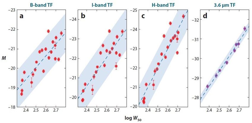
Abstract

       The Hubble constant is an important cosmological parameter that describes the expansion
rate of the universe. While it is not regarded as a fundamental parameter in standard cosmological
models, it can be measured by various independent methods and enables us to exploit the wealth of
observational data to advance our theoretical understanding in cosmology. We first review the
motivations for measuring the Hubble constant. We discuss how independent Hubble constant
measurements can break the geometrical degeneracy in cosmic microwave background
measurements so that one can precisely determine the spatial curvature and dark energy densities.
We also discuss how independent Hubble constant measurements can improve the constraints on
cosmological parameters derived from cosmic microwave background measurements, specifically
the equation of state for dark energy and the neutrino mass. Furthermore, we discuss the
application of the Hubble constant to predict the age of the universe, which can be compared
against independent estimates from stellar chronometry on the oldest stars and cosmic microwave
background measurements so as to validate our understanding on the underlying cosmology of the
universe. We then review various modern methods to measure the Hubble constant, focusing on
their underlying physics, major sources of systematic errors and recent results. Based on the Hubble
law, various distance methods have been devised to determine the Hubble constant via distance
measurements on different types of galactic objects. Among these, we discuss the currently most
powerful methods using Cepheids, type Ia supernovae, the tip of red giant branch, the Tully-Fisher
relation and surface brightness fluctuations, as well as a promising method using masers. Other
complementary, and potentially competitive, non-distance methods have been developed: we
discuss the methods based on baryon acoustic oscillations, Sunyaev-Zel’dovich effect, gravitational
lens time delays and gravitational waves. At present, the Hubble constant values predicted by
various methods span a wide range from low 60s to high 70s (km per second per mega-parsec), and
a more thorough physical understanding on the systematics affecting each method may be required
for the predicted values to converge. We suggest a reasonable and safe approach of adopting a
value derived from a combination of independent high quality measurements: a good set comprises
cosmic microwave background, Cepheid, type Ia supernova and baryon acoustic oscillations
measurements and gives the Hubble constant as                    km s-1 Mpc-1 (Komatsu et al. 2011).
Finally, we highlight the future developments in observational cosmology which are expected to
improve the accuracies of the various methods discussed to the 1-3% level.

                                                 2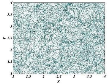
Contents

1.   Introduction                                                          6

2.   Motivations for Measuring the Hubble Constant                         13
     2.1   Physical Origins of CMB Anisotropies                            13
     2.2   Geometrical Degeneracy                                          16
     2.3   Constraining the Equation of State for Dark Energy              18
     2.4   Constraining the Neutrino Mass                                  21
     2.5   Age of the Universe                                             23

3.   Distance Methods to Measure the Hubble Constant                       25
     3.1   Cepheids                                                        25
           3.1.1   Physical Origin                                         25
           3.1.2   Observational Properties – the Leavitt Law              26
           3.1.3   Fundamental Techniques to Calibrate Cepheid Distances   28
           3.1.4   Main Sources of Systematic Errors                       30
     3.2   Type Ia Supernovae                                              32
           3.2.1   Observational Properties                                32
           3.2.2   Underlying Physics                                      35
     3.3   Recent Results for the Hubble Constant by Cepheid and Type Ia
           Supernova Distances                                             36
     3.4   Tip of the Red Giant Branch Method                              38
     3.5   Tully-Fisher Method                                             40
     3.6   Surface Brightness Fluctuations Method                          42
     3.7   Masers                                                          43
     3.8   Hubble Diagram based on Modern Distance Measurements            45

                                              3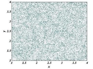
4.   Other Methods to Measure the Hubble Constant                                  48
     4.1   Baryon Acoustic Oscillations                                            48
           4.1.1   Physical Relation to the Hubble Constant                        48
           4.1.2   Error Sources                                                   50
           4.1.3   Recent Results for the Hubble Constant using BAO measurements   53
     4.2   Sunyaev-Zel’dovich Effect                                               54
           4.2.1   Inverse-Compton Scattering                                      55
           4.2.2   Thermal SZE                                                     58
           4.2.3   Other Types of SZE: Non-thermal, Kinematic and Polarization     59
           4.2.4   Method of Measuring the Hubble Constant via the SZE             61
           4.2.5   Major Systematics                                               63
           4.2.6   Recent Results for the Hubble Constant Measured via the SZE     66
     4.3   Gravitational Lens Time Delays                                          66
           4.3.1   Fundamental Principles                                          66
           4.3.2   Constraints, Degeneracies and Other Difficulties                69
           4.3.3   Recent Results for the Hubble Constant                          72
     4.4   Gravitational Waves                                                     73

5.   Conclusion                                                                    75

     Acknowledgements                                                              77

     Reference                                                                     78

                                             4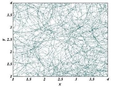
List of Figures

1.1   The original Hubble diagram                                                            7
2.1   Schematic representation of the CMB power spectrum for scale invariant adiabatic
      scalar models                                                                         14
2.2   Degeneracy lines in the            plane for a fixed                                  17
2.3   Likelihood ratio contours in the           plane for models containing only scalar
      modes                                                                                 18
2.4   Projected accuracies for the equation of state for dark energy due to improved
      CMB and Hubble constant measurements                                                  20
2.5   Improved constraint on the total mass of neutrinos due to independent Hubble
      constant measurements via baryon acoustic oscillations and supernovae                 22
3.1   The Cepheid manifold                                                                  28
3.2   Spectra of normal type Ia supernovae                                                  33
3.3   Light curves of SN 1992A observed at three wavelengths                                34
3.4   Red giant branch luminosity function of NGC 5253                                      39
3.5   Tully-Fisher relations at various wavelengths for galaxies calibrated with
      independent Cepheid measurements from the Hubble Space Telescope Key Project          41
3.6   Prototype H2O maser galaxy NGC 4258                                                   44
3.7   Hubble diagram based on modern distance measurements                                  46
4.1   Schematic diagram for the Alcock-Paczynski test                                       49
4.2   Schematic illustration of the correlation function and the power spectrum for
      baryon acoustic oscillations                                                          50
4.3   Peak broadening in the correlation function and damping in the power spectrum
      due to non-linear clustering                                                          53
4.4   Schematic galaxy distributions showing the effects due to peak broadening in the
      correlation function and damping in the power spectrum                                53
4.5   Sunyaev Zel’dovich effect (SZE) of a fictional cluster 1000 times more massive than
      a typical cluster                                                                     54
4.6   The spectral deformation caused by inverse-Compton scattering of an incident
      Planck spectrum after a single scattering from a thermal population of electrons as
      a function of dimensionless frequency                                                 57
4.7   Relative strengths of the thermal and kinematic Sunyaev Zel’dovich effects (SZE)      61
4.8   Basic ray geometry of gravitational lensing                                           67

                                                  5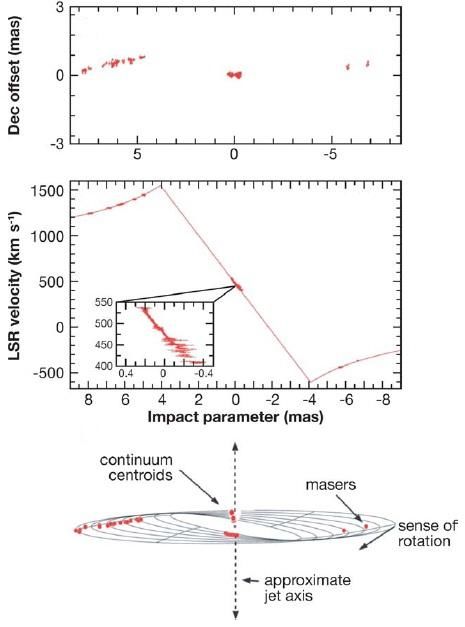
1. Introduction

        In 1929, Edwin Hubble discovered a linear correlation between the distance ( ) and

recessional velocity ( ) measurements of galaxies as far as the Virgo cluster (see Fig. 1.1 for the

original Hubble diagram):

                                                                                               (1.1)

This empirical relation (referred as the Hubble law) suggests that the more distant a galaxy is from us,

the faster it moves away from us. It provided the first piece of direct evidence for the expansion of

our universe (where spacetime itself is expanding) and prompted Einstein to abandon his attempts

to build a static universe model via the cosmological constant (which, however, would be re-

introduced later due to the inferred existence of dark energy). The proportionality factor (   ) in this

relation became to be known as the Hubble constant, and is a measure of the current expansion rate

of the universe. Its value as originally determined by Hubble (500 km s-1 Mpc-1) was almost an order

of magnitude larger than currently accepted values (around 70 km s-1 Mpc-1), due to significant

errors in the original distance measurements available to Hubble (Tammann 2005). Note that the

Hubble constant is often expressed numerically as , equal to         divided by 100 km s-1 Mpc-1; for

example, in the above            km s-1 Mpc-1 is equivalent to        .

        In practice, the recessional velocity can be determined accurately from the redshift ( ) of the

galaxy ( and     below refer to observed and emitted wavelengths respectively):

                                                                                               (1.2)

For small redshifts (       ),       and the Hubble law (eq. 1.1) can be expressed as                  .

However, for larger redshifts the relation between the recessional velocity and redshift is non-linear

and dependent on the cosmology (i.e. energy-matter contents) of the universe. The Hubble law can

then be re-expressed, using the Hubble parameter          , as:

                                                   6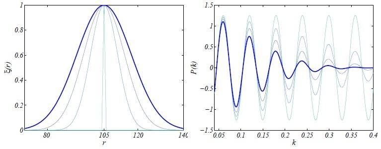
Fig. 1.1 – The original Hubble diagram (Hubble 1929): The recessional velocities and distances for
     46 galactic objects show a linear correlation (the Hubble law) with a constant of proportionality
                                               -1    -1
     (the Hubble constant) of around 500 km s Mpc , much larger than currently accepted values of
                    -1    -1
     around 70 km s Mpc due to significant errors in the original distance data.

                                                                                                    (1.3)

Note that      is simply the Hubble parameter as measured currently (              ). Also, in cosmology the

further we observe (larger ), the greater the redshift and the earlier the epoch of the universe we

are observing. A variable Hubble parameter essentially corresponds to a changing expansion rate

during the evolution of the universe, as determined by the dynamics of the energy-matter contents.

        Before Hubble’s empirical discovery, the expansion of the universe had already been

predicted through theoretical applications of General Relativity, independently by Alexandar

Friedmann in 1922 and Georges Lemaitre in 1927. For a homogeneous and isotropic universe

described by the Friedmann-Robertson-Walker (FRW) metric, the Einstein field equations lead to the

Friedmann equations (eq. 1.4a-b), and by defining the Hubble parameter                 in terms of a cosmic

scale factor      and its time-derivative , we have:

                                                     7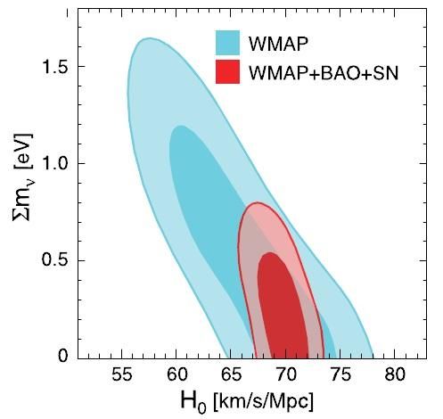
(1.4a)

                                                                                                   (1.4b)

The cosmic scale factor describes the relative size of the universe (         at present and         at the

Big Bang), thereby allowing the interpretation of the Hubble parameter                   as the expansion

rate.   and    refer to the density and pressure of individual energy-matter components labeled by

the subscript , each with its distinct equation of state                       reflecting its nature and

properties.    specifies the global spatial geometry of the universe (+1, 0, –1 for open, flat and closed

geometries respectively).

        Often the densities are expressed in units of the critical density                       (the total

energy-matter density below which an expanding universe without dark energy would eventually re-

collapse) as                   , so that eq. (1.4a) can be re-written as

                                                                                                   (1.4c)

where we have used the monotonic relationship between cosmic time and redshift of the FRW

universe to re-parameterize     in , while the spatial geometry of the universe has been expressed as

the curvature density                     (with           ). The subscript 0 indicates that the value is

taken at present. In general, we also have                                     . Current observations are

consistent with the standard concordance (ΛCDM) model with                        (matter consisting of a

small fraction of baryons and mostly cold dark matter),                    (dark energy in the form of a

cosmological constant,            ) and           (spatially flat). For details on the cosmological context,

the reader may refer to standard texts such as Dodelson (2003).

        The above theoretical relations (eq. 1.4a-c) describe how the energy-matter contents and

the geometry of the universe govern the evolution of the expansion rate. Crucially, they suggest that

information on the Hubble parameter, obtained by direct or indirect measurements, may help us

                                                     8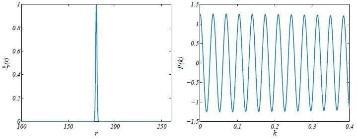
infer and better understand the underlying cosmology of the universe. Specifically, while high quality

measurements on the CMB anisotropies have enabled us to determine various cosmological

parameters with high precisions and accuracies, there exists a nearly exact geometrical degeneracy

that permits cosmological models with different values for          and     to agree with the same CMB

anisotropies. Thus, it is fundamentally impossible to determine the spatial curvature of the universe

solely from CMB measurements. To break this geometrical degeneracy, one can incorporate

independent measurements on the Hubble constant (             ) in the analysis of CMB measurements to

obtain constraints on      and     . Furthermore, independent         measurements of high accuracies

can complement CMB measurements to derive tighter constraints on other cosmological parameters

such as the equation of state for dark energy (where it is no longer assumed to be a cosmological

constant) and the neutrino mass. Another interesting application of               measurements is the

determination of the age of the universe, which depends on the underlying cosmology as well as the

expansion rate. Theoretical estimates based on            and an assumed cosmological model can be

compared against estimates from independent methods using stellar chronometry and CMB

measurements. Historically, the inconsistency between the predicted ages based on matter-

dominated models without dark energy (for any            values greater than 50 km s-1 Mpc-1) and stellar

chronometry applied to the oldest stars in the Milky Way had provided strong indication for the

existence of dark energy. These topics will be discussed further in Section 2 to provide some

motivations for measuring the Hubble constant.

        Most of the historical and modern observations to determine the Hubble constant employ

one or a combination of distance measurement methods. As the recessional velocity of a galaxy can

be accurately measured from the observed redshift, one can determine the Hubble constant (via the

Hubble law) essentially by measuring the distance to the galaxy. One can measure the angular

diameter distance      or the luminosity distance       , based on the simple facts that the more distant

an object is, the smaller and fainter it will appear to the observer. Quantitatively,

                                                    9
(1.5a)
(1.5b)
where are the proper size, apparent angular size (in radians), intrinsic luminosity and
observed flux (integrated over all wavelengths) respectively. They measure the true distance and are
related by . The relations above (eq. 1.5a-b) allow one to determine the relative
distance of the observed object. To determine directly the absolute distance, the intrinsic size or
luminosity of the observed object must be known – astrophysical objects as such are known as
‘standard rulers’ and ‘standard candles’ respectively. Various types of standard candles, such as
Cepheids and type Ia supernovae, exist in sufficient numbers across the universe from our own
galaxy to very distant galaxies. In addition, the absolute distance can be measured, using
trigonometric parallax, directly and accurately for objects very close or within our galaxy (less than 1
kpc away). Astrophysical objects for which we can directly determine the absolute distance are
primary distance indicators, while those that we have to calibrate, via the relative distance relations
eq. (1.5a-b), using known distances of primary indicators (located in the same galaxy hosts) are
known as secondary distance indicators. With astronomical observations accumulated over years,
one can construct a cosmic distance ladder, which is a succession of partially overlapping patches of
distance scales calibrated using various methods, to obtain the distances of nearby to very distant
galaxies (for a detailed review on galactic distance measurements, see Rowan-Robinson 1985).
Despite the seemingly simple underlying concept for the distance methods to determine the
Hubble constant, there exist sources of systematic errors that can severely affect the calibration of
the distance scales. Corrections for these errors are not straightforward especially where the
underlying physics is not well understood. Even if the same observational data is used, different
approaches to correct for possible systematics may result in widely inconsistent estimates of the
Hubble constant (as much as more than 15% difference). Nevertheless, distance measurement
methods continue to play a key role in Hubble constant measurements due to their advantages: the
relatively large number of observed galaxies where the methods can be applied; the availability of
10well established empirical calibration techniques in spite of imperfect theoretical understanding; and
the good consistency, in general, of their predictions with results obtained by other independent
methods (Section 4). In Section 3 we review the main modern distance methods: the uses of
Cepheids, type Ia supernovae, tip of the red giant branch and masers, as well as the Tully-Fisher and
surface brightness fluctuations methods. We focus on the underlying physics that enables the
distance measurement as well as the major systematics, and also highlight some recent results for
the Hubble constant as determined by these methods.
While the distance methods are empirically effective for the purpose of estimating the
Hubble constant, our theoretical understanding on the distance indicators is far from thorough,
rendering it difficult to ascertain the reliability of our calibration and error correction procedures in
using these distance indicators. Thus, we need other independent methods, ideally based on well
established physics, to provide alternative estimates of the Hubble constant so as to, hopefully,
confirm the validity of the results by a consistency check. As mentioned earlier, CMB anisotropies,
which are theoretically well understood, can be analyzed in conjunction with other independent
measurements (primarily to break the geometrical degeneracy) to derive a tight constraint on the
Hubble constant amongst constraints on other parameters. In addition, baryon acoustic oscillations
(BAO), which arise from the same process that produces the CMB radiation, provide a standard ruler
in the form of a characteristic length scale in the underlying matter distribution. Information on the
Hubble parameter is contained the radial mode of this characteristic length scale at different
redshifts, and hence we can derive the Hubble constant from BAO measurements. Another
independent method uses measurements of the Sunyaev-Zel’dovich effect (SZE) and the X-ray
emission due to galaxy clusters. This method crucially makes use of the different dependences on
electron density along the same path-length in the electron gas, to estimate the angular size and
therefore the angular diameter distance of the galaxy cluster. The Hubble constant can then be
obtained by combining this information with the measured redshift. Furthermore, gravitational
lensing can produce, from the same source, multiple images that have different propagation times
11to us. If the source luminosity varies in a regular manner, the relative time delays, which are
inversely proportional to the Hubble constant and dependent on the lens mass distribution, can be
used to derive the value of the Hubble constant. Lastly, gravitational waves from coalescing binary
systems provide a plausible means to determine the Hubble constant that is completely
independent of electromagnetic observations used in all of the previously mentioned methods. We
review these methods in Section 4.
Finally, in Section 5 we summarize the current outlook on the subject of Hubble constant
measurements; in particular, we briefly highlight some key on-going and future projects to obtain
improved measurements on the Hubble constant.
122. Motivations for Measuring the Hubble Constant
In this section we first review how accurate independent Hubble constant measurements
can be used in the analysis of high quality cosmic microwave background (CMB) data to improve
constraints on key cosmological parameters. We briefly recap the physical origins of CMB
anisotropies (Section 2.1), highlighting how their features are related to the underlying cosmological
parameters, and then discuss the applications of Hubble constant measurements to break the
geometrical degeneracy (Section 2.2) as well as to derive better constraints on the equation of state
for dark energy (Section 2.3) and the neutrino mass (Section 2.4). We also discuss the implications of
the Hubble constant on the predicted age of the universe (Section 2.5).
2.1 Physical Origins of CMB Anisotropies
The CMB is essentially formed by primordial photons that were released after recombination
(at approximately 3 × 10⁵ years after Big Bang, corresponding to a redshift ) and since then
have been largely free-streaming. While the CMB spectrum, i.e. its intensity as a function of
frequency and direction on the sky, is an extremely good blackbody with a nearly uniform
temperature in all directions (Fixsen et al. 1996), anisotropies exist. The underlying physical
mechanisms can be understood using linear perturbation theory, where anisotropies are generally
described in terms of temperature fluctuation and polarization (the latter is a higher order effect).
Prior to recombination, photons and baryons were tightly coupled due to Thomson and
Coulomb scattering. Initial density fluctuations in this photon-baryon fluid led to pressure gradients
which, together with competing gravitational forces, produced acoustic oscillations. Shortly after
recombination, photon-baryon decoupling occurred as the scattering rates became slower than the
accelerating rate of expansion of the universe. Thus, the CMB spectrum observed today captures the
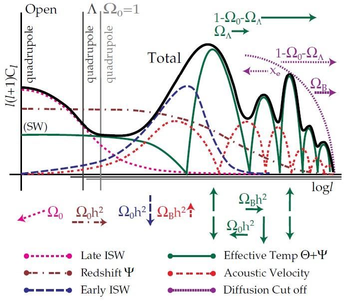
acoustic oscillations pattern as imprinted on the CMB photons at decoupling. Fig. 2.1 shows a
schematic representation of the CMB spectrum for scale invariant adiabatic scalar models.
13Fig. 2.1 – Schematic representation of the CMB power spectrum for scale invariant adiabatic scalar
models (Hu et al. 1997): This figure illustrates the various contributions to the overall CMB
spectrum (black solid curve ‘Total’) as discussed in Section 2.1. Note that ‘Effective Temp’ includes
the ‘Redshift’ contribution. Features in open models would be shifted to significantly smaller
angles compared with Λ and models, represented here as a shift in the axis beginning at
the quadrupole . The arrows show the dependence of each contribution on the cosmology.
For instance, a decrease in (subscript 0 in this figure refers to cold dark matter, for which we
use subscript m), corresponding to an increase in radiation content, enhances the ‘Early ISW’ and
thus broadens the first peak; furthermore it also impacts the peak heights via its effects on the
‘Effective Temp’. An increase in will enhance the odd peaks relative to the even peaks via the
‘Effective Temp’ and ‘Acoustic Velocity’ contributions. Similarly, other parameters affect the
profile of the CMB spectrum via various contributions (for details, refer to references within
Section 2.1). Note that in the figure above is the ionization fraction.
In Fig. 2.1, ‘Effective temperature’ refers to the anisotropies attributed to the Sachs-Wolfe
effect, due to acoustic oscillations of the photon-baryon fluid and gravitational redshifts of the
photons as they decouple from baryons and stream out of potential wells (the latter contribution is
14shown by the ‘redshift’ curve). The Sachs-Wolfe effect depends on the initial conditions of the
universe and the sound horizon , where is the conformal time at recombination and is the
speed of sound, which depends crucially on the baryon-photon density ratio as follows:
(2.1)
Meanwhile, the velocity profile associated with the acoustic oscillations of the photon-baryon fluid
also contributes to the anisotropies (the ‘acoustic velocity’ curve) via Doppler effect. However, this
contribution is small, though measurable, relative to that of the Sachs-Wolfe effect as it is
suppressed by the presence of even a tiny amount of baryons. Furthermore, there are contributions
from the integrated Sache-Wolfe (ISW) effect, which is caused by time-variations in the gravitational
potential and acts on the photons during their free-streaming from the last scattering surface to us.
‘Early ISW’ occurs before the matter domination phase of the expanding universe (after last
scattering) while ‘late ISW’ occurs after curvature or dark energy domination, and their contributions
to the CMB spectrum depend respectively on (early ISW) and or (late ISW). Lastly,
‘diffusion cutoff’ is a damping effect due to imperfect coupling between photons and baryons.
Photons diffuse over a length scale approximately proportional to and smoothen
out the anisotropies. This corresponds to the washing out of small scale (large ) features in Fig. 2.1.
Overall, the detailed profile of the CMB spectrum, such as the positions of its peaks and troughs, the
spacing between adjacent peaks and the locations of the peaks, is determined by (in decreasing
order of importance) the initial conditions and the contents of the universe before and after
recombination (via effects on various contributions as indicated in Fig. 2.1). As such, precise CMB
measurements allow us to derive tight constraints on four fundamental parameters (Hu & Dodelson
2002): the physical dark matter density ( ), the physical baryon density ( ), the comoving
angular diameter distance between recombination and present ( ) and the overall spectral tilt ( )
(Fig. 2.1 assumes ). Note that the third parameter contains information on curvature ( ) or
15dark energy ( ), while the fourth relates to the initial conditions. From these, other secondary
parameters, including the Hubble constant km s-1 Mpc-1), may be derived. For details on
the physics of CMB anisotropies, see e.g. Hu et al. (1997), Hu & Dodelson (2002) and Dodelson (2003)
(the first two for a more qualitative overview and the third for a more quantitative discussion).
2.2 Geometrical Degeneracy
Various degeneracies among cosmological parameters exist in the CMB anisotropies
(Efstathiou & Bond 1999). These parameter degeneracies span a wide range over the sensitivity to
CMB measurements, but most are, in principle, breakable if sufficiently precise measurements are
available. However, there is a nearly exact geometrical degeneracy such that CMB anisotropies alone,
when analyzed using linear perturbation theory, cannot distinguish models with different
background geometries but identical (non-dark energy) matter contents regardless of the precision
of the CMB measurements. Thus, this geometrical degeneracy imposes fundamental limits on how
well one can determine the curvature of the universe as well as the Hubble constant from CMB
anisotropies alone.
We recall from Section 2.1 that cosmological parameters describing the energy-matter
contents of the universe, i.e. physical densities ( ) of baryons, cold dark matter, curvature
and dark energy, have measurable effects on the CMB spectrum. Clearly, recalling
from Section 1, the physical densities obey the following constraint equation:
(2.2)
Physically, these parameters influence the CMB spectrum via two physical scales, the sound horizon
at recombination and the angular diameter distance to the last scattering surface. The former
depends on baryon and dark matter physical densities but not curvature or dark energy (since the
latter two are dynamically negligible at recombination). The latter depends on the combined
physical density of baryons and dark matter, as well as the physical densities of curvature and dark
16energy. The mapping from these parameters to the CMB spectrum is such that models with different
combinations of curvature and dark energy lead to indistinguishable features at high multipoles of
the spectrum, and hence the geometrical degeneracy. This is illustrated by the degeneracy lines in
Fig. 2.2. As illustrated by Fig. 2.3, a greater precision in CMB measurements merely corresponds to
narrowing around the degeneracy line without being able to rule out certain combinations of
curvature and dark energy. Thus, the geometrical degeneracy is fundamental, in the sense that it
cannot be broken by improving CMB observations alone. Note that at low multipoles curvature and
dark energy do result in distinguishable CMB features, but these differences are less significant than
the errors due to cosmic variance (i.e. limited sample size for large-scale measurements in a finite
universe), hence it is impossible to break the geometrical degeneracy from CMB anisotropies alone.
Fig. 2.2 – Degeneracy lines in the plane for a fixed (Efstathiou & Bond 1999): Each
degeneracy line is labeled by a parameter that depends on various component densities, and
represents the curvature and dark energy densities that would give rise to the same observed
CMB anisotropies given fixed total matter density ( ) and primordial fluctuation spectrum.
The five dots indicate models for which the baryon and cold dark matter densities ( and )
are, in fact, individually identical (i.e. not just their sum which is fixed along each degeneracy line);
despite their different curvature and dark energy densities, their CMB anisotropies would be
undistinguishable, illustrating the geometrical degeneracy.
17The constraint equation (eq. 2.2) implies that one may use independent constraints on the
Hubble constant (or dark energy), obtained from measurements other than the CMB spectrum, to
break the geometrical degeneracy. In particular, when the matter content parameters are well
constrained by CMB measurements, a constraint on the Hubble constant directly converts into a
constraint on dark energy. In general, . An accuracy of for can be
achieved if the errors on can be kept to 5% (Efstathiou & Bond 1999).
Fig. 2.3 – Likelihood ratio contours in the (physical densities) plane for models containing
only scalar modes (Efstathiou & Bond 1999): Similarly as Fig. 2.2, the solid curve is a degeneracy
line with a fixed parameter , and all models have identical baryon and cold dark matter densities
( and ). The (approximate) , and contours are generated from actual (but older)
observational data (refer to the original paper for details). Improved observational sensitivities
would allow one to zoom into contours of higher likelihood, but these regions still lie along the
degeneracy line and hence the geometrical degeneracy cannot be broken in this way.
2.3 Constraining the Equation of State for Dark Energy
Besides the cosmological constant ( ), other candidates for dark energy have been
proposed, e.g. cosmic strings ( ), domain walls ( ), quintessence (constant
or dynamical w). CMB measurements, when combined with other independent
18cosmological measurements, provide direct constraints on the dark energy equation of state. In fact,
Hu (2005) suggests that an independent Hubble constant measurement accurate to the percent
level is the single most useful complement to CMB parameters for dark energy studies. This appears
counter-intuitive because the Hubble constant is measured at present while the CMB is primarily a
snapshot of the last scattering surface where dark energy was subdominant. The essence of how this
works is that CMB anisotropies provide two self-calibrated (internally consistent) standards for dark
energy studies: the sound horizon at recombination and the initial amplitude of fluctuations at the
Mpc-1 scale. With the expansion history in the decelerating phase fixed according to the
standard thermal theory, deviations in the underlying CMB parameters due to the dark energy
equation of state are translated via the two standards into variations in the Hubble constant. With
current calibrations of the two standards using WMAP data alone at an accuracy of ≤4% and ≤10%
respectively, Hu (2005) concludes that a Hubble constant measurement with an accuracy of a few
percent can constrain the dark energy equation of state at a redshift around 0.5 to a comparable
fractional precision (assuming the universe is flat).
A few analytical estimates on the relation between errors in the Hubble constant and dark
energy parameters are provided by Olling (2007). Assuming a flat universe, the current Hubble
constant error of 9.8% contributes roughly half of the uncertainties in the dark energy parameters
(equation of state and density). However, data from the future Planck mission should result in an
eightfold decrease in the other half of the contributions, thus errors in the Hubble constant, if not
reduced significantly, would fully dominate the uncertainties in the dark energy parameters. On the
other hand, significant improvements in the accuracy of the Hubble constant (to 1% level) could
greatly improve the accuracy of the dark energy equation of state (to as good as 2%). Fig. 2.4 shows
the projections by Olling (2007) for future WMAP 8-year and Planck data. Aside, a Hubble constant
measurement with an accuracy at 1% level would decrease the error on the spatial curvature by a
factor 16. In addition, while improvements in the Hubble constant accuracy would eventually offer
19diminishing improvements in dark energy studies, Olling (2007) suggests that this approach is still
potentially more cost and time effective.
Fig. 2.4 – Projected accuracies for the equation of state for dark energy due to improved CMB and
Hubble constant measurements (Olling 2007): Results are obtained by using the approximate
linear relations between cosmological parameters by Spergel et al. (2007) and standard error-
propagation relations. The top panel shows the projected accuracies for the equation of state for
dark energy for various accuracies for CMB, represented by the four vertical lines corresponding
to (from left to right) WMAP 1-year, WMAP 3-year, WMAP 8-year and Planck data, as well as
Hubble constant measurements, represented by the four curves corresponding to (from top to
bottom) 10.8%, 5.4%, 2.7% and 1.1%. The error bars reflect the estimated variations if flatness is
not assumed (refer to the original paper for details). The bottom panel shows the contribution of
the errors in the Hubble constant to the total errors in the equation of state. The four vertical lines
represent the same accuracies for CMB while the four curves represent (from top to bottom)
-1 -1
errors in the Hubble constant of 8/1, 8/2, 8/4 and 8/10 km s Mpc respectively.
202.4 Constraining the Neutrino Mass
Despite their abundance in the universe, neutrinos have been difficult to study
experimentally due to their weak interactions. However, neutrino experiments have now established
that neutrinos have non-zero masses and provided constraints on the squared mass differences
between neutrino eigenstates. Furthermore, cosmology has turned out to be a fruitful area for
neutrino studies (see e.g. Crotty et al. 2004 and Hannestad 2006 for detailed reviews). Firstly,
neutrinos contribute to the overall relativistic energy density and play a key role in the evolution of
the universe during the radiation epoch. Neutrino properties affect the time of radiation-matter
equality and the sound horizon at decoupling, and impact mainly on the background (e.g. mean CMB
temperature) evolution. Secondly, neutrino masses determine the extent of their free-streaming and
therefore have implications on the evolution of cosmological fluctuations at the level of background
quantities and directly on the perturbations. Thus, cosmological observations can be used to derive
constraints on neutrino parameters.
An advantage of studying neutrinos through cosmology is that it can provide constraints on
the absolute mass of the neutrinos. Neutrinos affect the CMB spectrum when at least one of the
neutrino masses is greater than the mean energy of relativistic neutrinos per particle at so
that they would be non-relativistic at decoupling. This corresponds to a lower limit on neutrino mass
of eV. If the heaviest neutrino species is lighter than this, then CMB measurements
alone will not reveal any insights into neutrino masses. Supposing that neutrino mass eigenstates are
degenerate with an effective number of species of 3.04 (current standard value), CMB
measurements would be sensitive for total neutrino mass eV (Komatsu et al. 2009). To
probe below this value, one needs additional measurements independent of CMB, such as baryon
acoustic oscillations (BAO) or supernova (SN) data, to place a constraint on the neutrino mass.
The results of Komatsu et al. (2009) illustrate how measurements on the Hubble constant
can improve the constraints on the neutrino mass. Using WMAP 5-year data alone and adopting flat
21ΛCDM models, they find the constraints on as eV (for ) and eV (for
) respectively (both at 95% confidence level). When BAO and SNe data are added, the
constraints are improved significantly to eV (for ) and eV (for ). This
is due to the additional information on the Hubble constant provided by the BAO and SNe data
(Ichikawa et al. 2005). Physically, provided that neutrinos are still relativistic during decoupling,
enhances the early ISW effect that causes a shift in the first CMB peak to lower multipoles.
However, as this shift can be countered by a smaller Hubble constant value, there is a degeneracy
(an anti-correlation) between the neutrino mass and the Hubble constant. Thus, independent
Hubble constant measurements can help to break this degeneracy and improve the constraints on
neutrino masses. This is illustrated by Fig. 2.5.
Fig. 2.5 – Improved constraint on the total mass of neutrinos due to independent Hubble constant
measurements via baryon acoustic oscillations and supernovae (Komatsu et al. 2009): The joint
two-dimensional marginalized distributions of and (at 68% and 95 confidence levels) are
shown for the cases where WMAP only and WMAP+BAO+SN results are used respectively. The
much tighter constraint obtained from the latter is largely attributed to the independent distance
information from BAO (to be discussed in Section 4.1).
222.5 Age of the Universe
In principle, the age of the universe is determined by the underlying cosmology and the
current expansion rate of the universe (i.e. the Hubble Constant):
(2.3)
In the above the summation is over all energy-matter contents in the universe (including possibly
curvature) in the cosmological model adopted. Eq. (2.3) provides a theoretical prediction based on
the adopted values of the Hubble constant and other cosmological parameters. Alternatively,
observations on stellar evolution or CMB anisotropies, together with their well understood models,
can also be used to estimate the age of the universe. These independent methods should provide
consistent predictions on the age, and by demanding so one may gain insights on the underlying
cosmology as well as the value of the Hubble constant. Historically this has helped provide evidence
or motivation for the existence of dark energy: for a universe without dark energy, any Hubble
constant values greater than km s-1 Mpc-1 resulted in ages that were less than the age estimates
from the observed stellar evolution of the oldest stars in the Milky Way. Based on current commonly
adopted parameters of km s-1 Mpc-1, and , the age of the universe is
estimated to be Gyr (Freedman & Madore 2010).
Observations on the stellar evolution of the oldest stars in globular clusters in our galaxy
allow us to estimate their ages and place a lower limit on the Hubble constant. The age can be
estimated by three independent ways. First is by radioactive dating, where one uses spectroscopic
measurements on the abundance of thorium and uranium (for which the half-lives are known) in
metal-poor stars. Given an initial relative abundance of the two elements from theoretical modeling,
the age can be estimated (for a review, see Sneden et al. 2001). Second is by white dwarf cooling,
which occurs as energy loss from radiation is not replenished since white dwarfs are supported by
electron degeneracy pressure alone. The resulting drop in luminosity, among the faintest white
23dwarfs, allows one to estimate the age of the galaxy cluster (for a review, see Moehler & Bono 2008).
Third is through modeling the evolution of the temperature-luminosity distribution for a system of
stars. As the stars (of different masses) evolve, their individual temperature-luminosity profiles
change. The temperature-luminosity distribution for the system of stars matches the theoretical
distribution at only one time, thereby allowing one to estimate the age of the stellar system. For this
method, while any stars in the system can be included, main sequence stars have well understood
theoretical models and therefore provide the best age estimates. In particular, the main sequence
turnoff time scale (for the hydrogen supply in the core to be exhausted) can be most robustly
predicted. Using this method (with a separate estimate of the time from the Big Bang to the
formation of the globular clusters), Krauss & Chaboyer (2003) obtains a lower bound of 11.2 Gyr and
a best fit value of 13.4 Gyr (both at 95% confidence level) for the age of the universe. The other two
methods also provide similar estimates for the age of the universe, albeit with larger uncertainties
due to the greater difficulties in modeling the physical processes. Separately, CMB measurements
allow us to derive the Hubble constant and the age of the universe as secondary quantities via the
constraints on and the distance to the last scattering surface by peak heights and positions
respectively. Using WMAP 5-year data with Type Ia SN and BAO data, Komatsu et al. (2009) derives
an age of Gyr. The various methods mentioned have led to consistent predictions on the
age of the universe.
243. Distance Methods to Measure the Hubble Constant
In Section 1 we mention that the Hubble constant can essentially be determined via distance
measurements (angular or luminosity) on the receding galaxies due to the relative ease and accuracy
of measuring the recessional velocities via the redshifts. A cosmic distance ladder providing
distances from nearby to distant galaxies can be constructed from the wealth of observational data.
This is crucial for the accurate determination of the Hubble constant, as distance measurements
must be obtained from objects sufficiently far away (at least a few tens of Mpc) so that the
recessional velocities observed are dominated by the Hubble flow (i.e. cosmic expansion) rather than
peculiar motions due to local structures. Furthermore, a large sample used in building the distance
ladder helps to suppress the resulting statistical uncertainties. We also have calibration methods
with high degrees of internal consistency amenable to empirical tests for systematic errors. In
practice, however, various observational and theoretical challenges remain. Few objects are
sufficiently luminous to be well observed at cosmological distances into the Hubble flow. Calibration
techniques for various distance indicators do not always have a solid theoretical basis, thus there
can be severe systematic errors built up in various layers of the distance ladder. Nevertheless, a
number of traditional and modern methods remain effective and promising – Cepheid, type Ia
supernova, tip of giant red branch, maser, Tully-Fisher relation and surface brightness fluctuations.
In the following we discuss the physical origins of these distance indicators, the main underlying
physics as well as sources of systematics, and recent results for these methods.
3.1 Cepheids
3.1.1 Physical Origin
Cepheids provide a widely applicable and powerful means for measuring distances to nearby
galaxies due to the ease of discovering and identifying them and, crucially, the Leavitt law (Leavitt
1908) which is empirically and theoretically well established. Physically, Cepheids arise when
25massive stars have exhausted the hydrogen in their cores and evolve rapidly back and forth across
the Hertzsprung-Russell (HR) diagram (in the instability strip). The Cepheid has a doubly-ionized
helium layer that acts like a heat engine and valve mechanism. When this ionized layer is opaque to
radiation, energy is trapped and the pressure within increases. As a result, this layer expands and
loses temperature, allowing recombination to occur and therefore causing a decrease in opacity.
More radiation then escapes through the layer and the reverse process occurs. This cycle repeats to
give rise to the observable periodic changes in the Cepheid luminosity (Freedman & Madore 2010;
for details, see Cox 1980).
3.1.2 Observational Properties – the Leavitt Law
The Leavitt law is a relation between the pulsation period, intrinsic luminosity and color. A
simple explanation (following Madore & Freedman 1991 and Rowan-Robinson 1985) is outlined
below. The pulsation period for a Cepheid is related to the natural oscillation period of the star,
which can be shown to be proportional to where is the mean density of the star. As the
natural oscillation period is essentially the time taken for the star to collapse if pressure support
were suddenly removed, one expects:
(3.1)
where is the pulsational constant (which depends on the manner at which pulsation occurs), while
and are the mass and radius of the star respectively. The luminosity of the star is related to its
effective temperature by the Stefan-Boltzmann law:
(3.2)
where is the Stefan-Boltzmann constant. For observational purposes, we describe the luminosity
by the corresponding magnitude or the absolute magnitude (the latter is the magnitude as
observed if the star were at a distance of 10 pc):
26(3.3a)
(3.3b)
where is a constant (which depends on the wavelength band at which the observations are made)
and is the distance to the star. Furthermore, over the mass range of Cepheids the following
relations may also be applied:
(3.4a)
(3.4b)
(3.4c)
In the above (eq. 3.4a-c), are just constants to be determined empirically or theoretically. is
the bolometric magnitude which describes the integrated effect over all wavelengths, unlike
magnitude which usually involves only a narrow wavelength band. refers to the color, defined
by astronomers as the ratio of fluxes at two different wavelengths (the usual notation is e.g.
where the letters specify the wavelength bands). The above relations (eq. 3.1-4) lead to the
following form of the Leavitt law ( are constants to be determined empirically or theoretically):
(3.5)
As hydrostatic equilibrium can be maintained for a long time along the core-helium-burning main
sequence, the Cepheids are constrained by the above (linearized) period-luminosity-color relation
(eq. 3.5) most of the time, hence enabling distance measurements using Cepheid observations. The
Cepheid manifold in Fig. 3.1 illustrates this period-luminosity-color relation.
27Fig. 3.1 – The Cepheid manifold (Madore & Freedman 1991): The PLC plane corresponds to the
instability strip in the Hertzsprung-Russell diagram where Cepheids reside. Here, represents
the period (c.f. eq. 3.5), represents the luminosity (c.f. eq. 3.3b) and represents the
color (c.f. eq. 3.4c). Projections on various two-dimensional planes (i.e. keeping one variable
constant) are also shown.
3.1.3 Fundamental Techniques to Calibrate Cepheid Distances
Since our main motivation for galactic distance measurements is to obtain independent
constraints on the Hubble constant which can serve either as a consistency test on values obtained
by other methods or as additional inputs to CMB measurements to improve the derived constraints
on degenerate cosmological parameters, one would ideally adopt distance calibration techniques
that are fundamental in a geometrical sense. However, all known Galactic Cepheids are more than
250 pc away; historically, their distances could only be determined using non-fundamental
techniques which depend upon statistical parallaxes or the presence of Cepheids in galactic clusters.
28Fortunately, recent progress has led to the development of fundamental techniques that allow us to
calibrate the Cepheid distance-luminosity relation geometrically or quasi-geometrically (the latter
refers to cases where there are non-geometric complications) (Barnes 2009).
Among these, a reliable method for finding Cepheid distances in our galaxy is the infrared
surface brightness method. The Baade-Wesselink method (Baade 1926; Wesselink 1946, 1969)
allows one to determine the mean radius of a Cepheid from its magnitude differences across
multiple phases, given its radial velocity curve. The correlation between the surface brightness and
color, established historically for non-variable stars and recently for Cepheids as well, allows one to
determine the mean surface brightness. Combining these, one can then determine the absolute
surface brightness of the Cepheid. The infrared color index is now commonly used as it is
the most effective in reducing uncertainties. In practice, such color computations require some
interpolation scheme based on accurate period information since V and K photometric data are
seldom collected simultaneously. The equations for finding distance and radius from magnitude,
color and radial velocity can now be solved rigorously and objectively using a Bayesian Markov-Chain
Monte Carlo code due to Barnes et al. (2003).
An alternative is the interferometric pulsation method which uses the observed
interferometric fringe patterns to deduce the angular diameter distance over a pulsation cycle. This
method requires an assumed model for the light distribution of the source, usually a uniform
intensity disk, and a theoretically established limb-darkening curve. Furthermore, it requires a
systematic correction in the form of a p-factor, which accounts for the difference between the
observed radial velocity and the actual pulsation velocity due to effects such as geometrical
projection, limb-darkening, choice of measurement technique, choice of lines measured and spectral
resolution. In fact, this p-factor correction is also needed in the surface brightness method. In this
sense, both methods discussed are quasi-geometric. The interferometric pulsation method does not
use color information and is therefore immune to reddening (discussed in Section 3.1.4). It is also
29potentially more precise than the surface brightness method, but is limited by the relatively smaller
sample size within the distance where the method can be applied. Nevertheless, it has so far been
useful as a check on the infrared surface brightness distance scale and for finding the p-factor
observationally. Finally, distance measurements of a farther range and a higher precision can be
obtained using trigonometric parallaxes by space missions. Cepheid distances determined by the
previous two techniques agree well with high quality Hubble Space Telescope (HST) data.
3.1.4 Main Sources of Systematic Errors
Error sources in Cepheid distance measurements include statistical (random) errors, which
manifest as the scatter in the period-luminosity relation (observed at a specific color), and various
systematic effects, among which the most significant contributions arise from reddening and
metallicity. Empirically Cepheid data do not follow the ideal (linearized) period-luminosity-color
relation (eq. 3.5), with individual deviations as high as equivalent to a distance error of 30%.
Fortunately, since statistical errors vary inversely with the square root of the sample size, these can
be reduced to 10% with as few as a dozen of Cepheids (Freedman & Madore 2010). Observationally,
the importance of the Magellanic Clouds for the calibration of the cosmic distance ladder is precisely
due to their closeness to us and the large numbers of Cepheids observed in them.
A key source of systematic errors that affect all distance indicators is the reddening effect
(alternatively known as interstellar extinction) which must be corrected before any meaningful
analysis on the observational data can be made. Reddening refers to the wavelength-dependent
absorption and scattering (re-emission) of photons, and it occurs in the parent galaxy of the objects
observed, along the line-of-sight and within our galaxy. It introduces systematic errors into the
derived distances since the observed object will appear fainter and farther than it actually is. If one
collects data at least two wavelength bands (say, V and I) and adopts, as a priori, a value for the ratio
of total-to-selective absorption , then the reddening effect can be incorporated into the constant
in the magnitude relations (eq. 3.3a-b):
30(3.6)
where is the color excess (defined as the difference between the observed and intrinsic
color indices) obtained from observational data. One can then obtain the Wesenheit magnitude:
(3.7)
which is by construction equivalent to the intrinsic Wesenheit magnitude on the right in eq. (3.7)
(computed using intrinsic values as denoted by subscript 0) and therefore free of reddening. While
this correction technique may break down in regions of intense star formation and extremely high
optical depths, Cepheids are generally sufficiently displaced from such regions for this correction to
be applicable. An alternative technique to minimize reddening is to observe at the longest
wavelengths possible, which is conceptually more robust but practically more challenging.
Besides reddening, another key source of systematic errors is due to the metallicity of the
observed objects. Differences in metal abundance in the stellar chemical compositions affect the
overall stellar structure and the corresponding properties such as color, brightness and radius of the
star. Theoretical studies on how metallicity impacts the period-luminosity relation have so far been
inconclusive. Empirically, two tests of the metallicity-dependence of the period-luminosity relation
have been used for samples in various galaxies. The first test uses measured radial metallicity
gradients within individual galaxies to determine the systematic errors solely due to metallicity. The
second test compares the Cepheid and tip of the red giant branch distance measurements for same
galaxies so as to establish the correlation of these differences with the metallicity. As results are still
being debated, this is very much an active area of research. In practice, as Section 3.3 illustrates
further, significant discrepancies can arise when different correction techniques are applied in the
calibration of distant galactic distances using nearby galactic distances where the galactic
metallicities are largely dissimilar (e.g. majority of the HST Key Project galaxies have metallicities
more comparable to our galaxy than the Large Magellanic Cloud but calibration was done using the
latter). For detailed reviews, see Madore & Freedman (1991) and Freedman & Madore (2010).
313.2 Type Ia Supernovae
Type Ia supernovae (SNe Ia) provide the most accurate distance measurements well into the
Hubble flow and is therefore a key distance indicator for measuring the Hubble constant. While our
theoretical understanding on SNe Ia is far from robust, observationally SNe Ia are bright enough to
be observed at great cosmological distances, can be reliably identified and exhibit a correlation of
very low intrinsic scatter between their peak luminosities and rates of decline so that they are good
standard candles. SNe Ia are primary distance indicators in the sense that their distances can be
estimated directly by the Baade-Wesselink method (Baade 1926; Wesselink 1946, 1969). Observing
the time-variation of the supernova luminosity and color, one can deduce the quantity
, where is the radius of the supernova photosphere at time and is the
radius at the instant of maximum luminosity. Using the radial velocity from the measured redshift,
one can then infer the value of . Putting this and the effective supernova temperature inferred
from the observed color into the Stefan-Boltzmann law (eq. 3.2), the maximum intrinsic supernova
luminosity can be determined (Rowan-Robinson 1985). Alternatively, distances of distant SNe Ia are
also calibrated using well measured Cepheid distances in nearby galaxies where both Cepheids and
SNe Ia are observed. In following we discuss the observational properties that make SNe Ia good
standard candles (Section 3.2.1) and our theoretical understanding on SNe Ia (Section 3.2.2).
3.2.1 Observational Properties
SNe Ia can be reliably identified by their spectra, light-curve shapes, colors and magnitudes.
Improved observational data reveal that SNe Ia are not strictly homogeneous, and a readily
distinguishable minority is classified as peculiar SNe Ia. Nevertheless, the majority classified as
normal SNe Ia displays a high degree of homogeneity and remains useful for distance measurements
to determine the Hubble constant.
32Spectra of normal SNe Ia can be distinguished unambiguously (except at high redshifts) by
their characteristic spectral evolution. The spectrum initially shows P Cygni lines of Si II, Ca II, S II, O I
and Mg II prior to and near maximum luminosity. Shortly after, blends of P Cygni permitted Fe II lines
are developed. Finally blends of forbidden emission lines of iron and cobalt ions are developed
during the late nebular phase. Fig. 3.2 provides an illustration. Quantitatively, the SN Ia spectra can
be analyzed by measuring the blueshifts of the absorption features or monochromatic flux ratios.
Various parameters have been defined for this purpose, e.g. Fisher et al. (1995) use a parameter
based on the wavelength of the red edge of the Ca II H&K absorption feature at moderately
late times and intended as a measure of the minimum ejection velocity of calcium; Branch & van den
Bergh (1993) use a parameter corresponding to the blueshift at 10 days after maximum
luminosity. Peculiar SNe Ia tend to have parameter values widely different from those of normal SNe
Ia, and hence can be clearly separated.
Fig. 3.2 – Spectra of normal type Ia supernovae (Branch 1998): The left panel shows the nonlocal
thermodynamic equilibrium spectra computed for a composition structure of model W7, 15 days
after explosion and a range of effective temperatures. The right panel shows the observed spectra
of six SNe Ia near maximum luminosity. The unique spectral features, as shown, enable us to
unambiguously identify type Ia supernovae provided that observations are of a decent quality.
33You can also read