Radiometric Dating A Christian Perspective
←
→
Page content transcription
If your browser does not render page correctly, please read the page content below
Radiometric Dating
                                A Christian Perspective
                                       Dr. Roger C. Wiens
                                      RCWiens@MSN.Com

Dr. Wiens has a PhD in Physics, with a minor in Geology. His PhD thesis was on isotope ratios in
meteorites, including surface exposure dating. He was employed at Caltech’s Division of
Geological & Planetary Sciences at the time of writing the first edition. He is presently employed in
the Space & Atmospheric Sciences Group at the Los Alamos National Laboratory

               Home address: 941 Estates Drive, Los Alamos, NM 87544

               First edition 1994; revised version 2002

               Radiometric dating--the process of determining the age of rocks from
               the decay of their radioactive elements--has been in widespread use
               for over half a century. There are over forty such techniques, each
               using a different radioactive element or a different way of measuring
               them. It has become increasingly clear that these radiometric dating
               techniques agree with each other and as a whole, present a coherent
               picture in which the Earth was created a very long time ago. Further
               evidence comes from the complete agreement between radiometric
               dates and other dating methods such as counting tree rings or glacier
               ice core layers. Many Christians have been led to distrust radiometric
               dating and are completely unaware of the great number of laboratory
               measurements that have shown these methods to be consistent. Many
               are also unaware that Bible-believing Christians are among those
               actively involved in radiometric dating.

               This paper describes in relatively simple terms how a number of the
               dating techniques work, how accurately the half-lives of the
               radioactive elements and the rock dates themselves are known, and
               how dates are checked with one another. In the process the paper
               refutes a number of misconceptions prevalent among Christians
               today. This paper is available on the web via the American Scientific
               Affiliation and related sites to promote greater understanding and
               wisdom on this issue, particularly within the Christian community.
Radiometric Dating
                                                           A Christian Perspective

                                                              Dr. Roger C. Wiens

                                                          TABLE OF CONTENTS

Introduction...............................................................................................................................................1
Overview...................................................................................................................................................1
The Radiometric Clocks...........................................................................................................................3
Examples of Dating Methods for Igneous Rocks ...................................................................................4
        Potassium-Argon .........................................................................................................................4
        Argon-Argon................................................................................................................................5
        Rubidium-Strontium....................................................................................................................6
        Samarium-Neodymium, Lutetium-Hafnium, and Rhenium-Osmium......................................9
        Uranium-Lead..............................................................................................................................9
The Age of the Earth ..............................................................................................................................10
Extinct Radionuclides: The Hourglasses that Ran Out .......................................................................11
Cosmogenic Radionuclides: Carbon-14, Beryllium-10, Chlorine-36 ................................................12
Radiometric Dating of Geologically Young Samples ..........................................................................15
Non-Radiogenic Dating Methods for the Past 100,000 Years.............................................................16
        Ice Cores.....................................................................................................................................16
        Varves ........................................................................................................................................17
        Other Annual-Layering Methods..............................................................................................18
        Thermoluminescence.................................................................................................................18
        Electron Spin Resonance...........................................................................................................18
        Cosmic Ray Exposure Dating...................................................................................................18
Can We Really Believe the Dating Systems? .......................................................................................19
Doubters Still Try...................................................................................................................................20
Apparent Age?........................................................................................................................................21
Rightly Handling the Word of Truth .....................................................................................................22

Appendix: Common Misconceptions Regarding Radiometric Dating Techniques...........................23
Resources on the Web............................................................................................................................28
Further Reading: Books ........................................................................................................................29
Acknowledgements ................................................................................................................................31
More About the Author..........................................................................................................................31
Glossary ..................................................................................................................................................32

                                                                             ii
Introduction
Arguments over the age of the Earth have sometimes been divisive for people who regard the Bible as
God’s word. Even though the Earth's age is never mentioned in the Bible, it is an issue because those who
take a strictly literal view of the early chapters of Genesis can calculate an approximate date for the
creation by adding up the life-spans of the people mentioned in the genealogies. Assuming a strictly literal
interpretation of the week of creation, even if some of the generations were left out of the genealogies, the
Earth would be less than ten thousand years old. Radiometric dating techniques indicate that the Earth is
thousands of times older than that--approximately four and a half billion years old. Many Christians
accept this and interpret the Genesis account in less scientifically literal ways. However, some Christians
suggest that the geologic dating techniques are unreliable, that they are wrongly interpreted, or that they
are confusing at best. Unfortunately, much of the literature available to Christians has been either
inaccurate or difficult to understand, so that confusion over dating techniques continues.
The next few pages cover a broad overview of radiometric dating techniques, show a few examples, and
discuss the degree to which the various dating systems agree with each other. The goal is to promote
greater understanding on this issue, particularly for the Christian community. Many people have been led
to be skeptical of dating without knowing much about it. For example, most people don't realize that
carbon dating is only rarely used on rocks. God has called us to be "wise as serpents" (Matt. 10:16) even
in this scientific age. In spite of this, differences still occur within the church. A disagreement over the age
of the Earth is relatively minor in the whole scope of Christianity; it is more important to agree on the
Rock of Ages than on the age of rocks. But because God has also called us to wisdom, this issue is worthy
of study.
Overview
Rocks are made up of many individual crystals, and each crystal is usually
made up of at least several different chemical elements such as iron,
magnesium, silicon, etc. Most of the elements in nature are stable and do not
change. However, some elements are not completely stable in their natural
state. Some of the atoms eventually change from one element to another by a
process called radioactive decay. If there are a lot of atoms of the original
element, called the parent element, the atoms decay to another element, called
the daughter element, at a predictable rate. The passage of time can be charted
by the reduction in the number of parent atoms, and the increase in the
number of daughter atoms.
Radiometric dating can be compared to an hourglass. When the glass is turned
over, sand runs from the top to the bottom. Radioactive atoms are like
individual grains of sand—radioactive decays are like the falling of grains
from the top to the bottom of the glass. You cannot predict exactly when any one particular grain will get
to the bottom, but you can predict from one time to the next how long the whole pile of sand takes to fall.
Once all of the sand has fallen out of the top, the hourglass will no longer keep time unless it is turned
over again. Similarly, when all the atoms of the radioactive element are gone, the rock will no longer keep
time (unless it receives a new batch of radioactive atoms).
1Unlike the hourglass, where the amount of
sand falling is constant right up until the end,
the number of decays from a fixed number of
radioactive atoms decreases as there are
fewer atoms left to decay (see Figure 1). If it
takes a certain length of time for half of the
atoms to decay, it will take the same amount
of time for half of the remaining atoms, or a
fourth of the original total, to decay. In the
next interval, with only a fourth remaining,
only one eighth of the original total will
decay. By the time ten of these intervals, or
half-lives, has passed, less than one
thousandth of the original number of
radioactive atoms is left. The equation for the
fraction of parent atoms left is very simple.
The type of equation is exponential, and is
related to equations describing other well-
known phenomena such as population
growth. No deviations have yet been found
from this equation for radioactive decay.
Also unlike the hourglass, there is no way to
change the rate at which radioactive atoms
decay in rocks. If you shake the hourglass,
twirl it, or put it in a rapidly accelerating
vehicle, the time it takes the sand to fall will
change. But the radioactive atoms used in
dating techniques have been subjected to
heat, cold, pressure, vacuum, acceleration, Figure 1. The rate of loss of sand from the top of an hourglass
and strong chemical reactions to the extent compared to the exponential type of decay of radioactive elements.
that would be experienced by rocks or Most processes we are familiar with are linear, like sand in the
magma in the mantle, crust, or surface of the hourglass. In exponential decay the amount of material decreases by
Earth or other planets without any significant half during each half-life. After two half-lives only one fourth is left,
change in their decay rate.1 after three half-lives only an eighth is left, etc. As shown in the
bottom panel, the daughter element or isotope amount increases
rapidly at first and more slowly with each succeeding half-life.
An hourglass will tell time correctly only if it
is completely sealed. If it has a hole allowing the sand grains to escape out the side instead of going
through the neck, it will give the wrong time interval. Similarly, a rock that is to be dated must be sealed
against loss or addition of either the radioactive daughter or parent. If it has lost some of the daughter
element, it will give an inaccurately young age. As will be discussed later, most dating techniques have
very good ways of telling if such a loss has occurred, in which case the date is thrown out (and so is the
rock!).
1
In only a couple of special cases have any decay rates been observed to vary, and none of these
special cases apply to the dating of rocks as discussed here. These exceptions are discussed later.
2An hourglass measures how much time has passed since it was turned over. (Actually it tells when a
specific amount of time, e.g., 2 minutes, an hour, etc., has passed, so the analogy is not quite perfect.)
Radiometric dating of rocks also tells how much time has passed since some event occurred. For igneous
rocks the event is usually its cooling and hardening from magma or lava. For some other materials, the
event is the end of a metamorphic heating event (in which the rock gets baked underground at generally
over a thousand degrees Fahrenheit), the uncovering of a surface by the scraping action of a glacier, the
chipping of a meteorite off of an asteroid, or the length of time a plant or animal has been dead.
The Radiometric Clocks
Table I Some Naturally-Occurring Radioactive Isotopes and
There are now well over forty
Their Half-Lives
different radiometric dating
techniques, each based on a Radioactive Isotope Product Half-Life
different radioactive isotope.2 A (Parent) (Daughter) (Years)
partial list of the parent and
daughter isotopes and the decay Samarium-147 Neodymium-143 106 billion
half-lives is given in Table I.
Notice the large range in the half- Rubidium-87 Strontium-87 48.8 billion
lives. Isotopes with long half-lives Rhenium-187 Osmium-187 42 billion
decay very slowly, and so are
useful for dating correspondingly Lutetium-176 Hafnium-176 38 billion
ancient events. Isotopes with
shorter half-lives cannot date very Thorium-232 Lead-208 14 billion
ancient events because all of the Uranium-238 Lead-206 4.5 billion
atoms of the parent isotope would
have already decayed away, like Potassium-40 Argon-40 1.26 billion
an hourglass left sitting with all
the sand at the bottom. Isotopes Uranium-235 Lead-207 0.7 billion
with relatively short half-lives are Beryllium-10 Boron-10 1.52 million
useful for dating correspondingly
shorter intervals, and can usually Chlorine-36 Argon-36 300,000
do so with greater accuracy, just
as you would use a stopwatch Carbon-14 Nitrogen-14 5715
rather than a grandfather clock to Uranium-234 Thorium-230 248,000
time a 100 meter dash. On the
other hand, you would use a Thorium-230 Radium-226 75,400
calendar, not a clock, to record
time intervals of several weeks or Most half-lives taken from Holden, N.E. (1990) Pure Appl.
more. Chem. 62, 941-958.
The half-lives have all been measured directly either by using a radiation detector to count the number of
atoms decaying in a given amount of time from a known amount of the parent material, or by measuring
2
The term isotope subdivides elements into groups of atoms that have the same atomic weight.
For example carbon has isotopes of weight 12, 13, and 14 times the mass of a nucleon, referred to as
carbon-12, carbon-13, or carbon-14 (abbreviated as 12C, 13C, 14C). It is only the carbon-14 isotope
that is radioactive. This will be discussed further in a later section.
3the ratio of daughter to parent atoms in a sample that originally consisted completely of parent atoms.
Work on radiometric dating first started shortly after the turn of the 20th century, but progress was
relatively slow before the late forties. However, by now we have had over fifty years to measure and re-
measure the half-lives for many of the dating techniques. Very precise counting of the decay events or the
daughter atoms can be done, so while the number of, say, rhenium-187 atoms decaying in 50 years is a
very small fraction of the total, the resulting osmium-187 atoms can be very precisely counted. For
example, recall that only one gram of material contains over 1021 (1 with 21 zeros behind) atoms. Even
if only one trillionth of the atoms decay in one year, this is still millions of decays, each of which can
be counted by a radiation detector!
The uncertainties on the half-lives given in the table are all very small. All of the half-lives are known to
better than about two percent except for rhenium (5%), lutetium (3%), and beryllium (3%). There is no
evidence of any of the half-lives changing over time. In fact, as discussed below, they have been observed
to not change at all over hundreds of thousands of years.
Examples of Dating Methods for Igneous Rocks
Now let's look at how the actual dating methods work. Igneous rocks are good candidates for dating.
Recall that for igneous rocks the event being dated is when the rock was formed from magma or lava.
When the molten material cools and hardens, the atoms are no longer free to move about. Daughter atoms
that result from radioactive decays occurring after the rock cools are frozen in the place where they were
made within the rock. These atoms are like the sand grains accumulating in the bottom of the hourglass.
Determining the age of a rock is a two-step process. First one needs to measure the number of daughter
atoms and the number of remaining parent atoms and calculate the ratio between them. Then the half-life
is used to calculate the time it took to produce that ratio of parent atoms to daughter atoms.
However, there is one complication. One cannot always assume that there were no daughter atoms to
begin with. It turns out that there are some cases where one can make that assumption quite reliably. But
in most cases the initial amount of the daughter product must be accurately determined. Most of the time
one can use the different amounts of parent and daughter present in different minerals within the rock to
tell how much daughter was originally present. Each dating mechanism deals with this problem in its own
way. Some types of dating work better in some rocks; others are better in other rocks, depending on the
rock composition and its age. Let's examine some of the different dating mechanisms now.
Potassium-Argon. Potassium is an abundant element in the Earth's crust. One isotope, potassium-40, is
radioactive and decays to two different daughter products, calcium-40 and argon-40, by two different
decay methods. This is not a problem because the production ratio of these two daughter products is
precisely known, and is always constant: 11.2% becomes argon-40 and 88.8% becomes calcium-40. It is
possible to date some rocks by the potassium-calcium method, but this is not often done because it is hard
to determine how much calcium was initially present. Argon, on the other hand, is a gas. Whenever rock is
melted to become magma or lava, the argon tends to escape. Once the molten material hardens, it begins
to trap the new argon produced since the hardening took place. In this way the potassium-argon clock is
clearly reset when an igneous rock is formed.
In its simplest form, the geologist simply needs to measure the relative amounts of potassium-40 and
argon-40 to date the rock. The age is given by a relatively simple equation:
t = h x ln[1 + (argon-40)/(0.112 x (potassium-40))]/ln(2)
where t is the time in years, h is the half-life, also in years, and ln is the natural logarithm.
4However, in reality there is often a small amount of argon remaining in a rock when it hardens. This is
usually trapped in the form of very tiny air bubbles in the rock. One percent of the air we breathe is argon.
Any extra argon from air bubbles may need to be taken into account if it is significant relative to the
amount of radiogenic argon (that is, argon produced by radioactive decays). This would most likely be the
case in either young rocks that have not had time to produce much radiogenic argon, or in rocks that are
low in the parent potassium. One must have a way to determine how much air-argon is in the rock. This is
rather easily done because air-argon has a couple of other isotopes, the most abundant of which is argon-
36. The ratio of argon-40 to argon-36 in air is well known, at 295. Thus, if one measures argon-36 as well
as argon-40, one can calculate and subtract off the air-argon-40 to get an accurate age.
Some young-Earth proponents recently
One of the best ways of showing that an age-date is correct is reported that rocks were dated by the
to confirm it with one or more different dating method(s). potassium-argon method to be a several
Although potassium-argon is one of the simplest dating million years old when they are really only a
methods, there are still some cases where it does not agree few years old. But the potassium-argon
with other methods. When this does happen, it is usually method, with its long half-life, was never
because the gas within bubbles in the rock is from deep intended to date rocks only 25 years old.
underground rather than from the air. This gas can have a These people have only succeeded in correctly
higher concentration of argon-40 escaping from the melting showing that one can fool a single radiometric
of older rocks. This is called parentless argon-40 because its dating method when one uses it improperly.
The false radiometric ages of several million
parent potassium is not in the rock being dated, and is also years are due to parentless argon, as described
not from the air. In these slightly unusual cases, the date here, and first reported in the literature some
given by the normal potassium-argon method is too old. fifty years ago. Note that it would be
However, scientists in the mid-1960s came up with a way extremely unlikely for another dating method
around this problem, the argon-argon method, discussed in to agree on these bogus ages. Getting
the next section. agreement between more than one dating
method is a recommended practice.
Argon-Argon. Even though it has been around for nearly
half a century, the argon-argon method is seldom discussed by groups critical of dating methods. This
method uses exactly the same parent and daughter isotopes as the potassium-argon method. In effect, it is
a different way of telling time from the same clock. Instead of simply comparing the total potassium with
the non-air argon in the rock, this method has a way of telling exactly what and how much argon is
directly related to the potassium in the rock.
In the argon-argon method the rock is placed near the center of a nuclear reactor for a period of hours. A
nuclear reactor emits a very large number of neutrons, which are capable of changing a small amount of
the potassium-39 into argon-39. Argon-39 is not found in nature because it has only a 269-year half-life.
(This half-life doesn't affect the argon-argon dating method as long as the measurements are made within
about five years of the neutron dose). The rock is then heated in a furnace to release both the argon-40 and
the argon-39 (representing the potassium) for analysis. The heating is done at incrementally higher
temperatures and at each step the ratio of argon-40 to argon-39 is measured. If the argon-40 is from decay
of potassium within the rock, it will come out at the same temperatures as the potassium-derived argon-39
and in a constant proportion. On the other hand, if there is some excess argon-40 in the rock it will cause
a different ratio of argon-40 to argon-39 for some or many of the heating steps, so the different heating
steps will not agree with each other.
5Figure 2 is an example of a good argon-
argon date. The fact that this plot is flat
shows that essentially all of the argon-40 is
from decay of potassium within the rock.
The potassium-40 content of the sample is
found by multiplying the argon-39 by a
factor based on the neutron exposure in the
reactor. When this is done, the plateau in
the figure represents an age date based on
the decay of potassium-40 to argon-40.
There are occasions when the argon-argon
dating method does not give an age even if
there is sufficient potassium in the sample
and the rock was old enough to date. This
most often occurs if the rock experienced a
high temperature (usually a thousand
degrees Fahrenheit or more) at some point Figure 2. A typical argon-argon dating plot. Each small rectangle
represents the apparent age given at one particular heating-step
since its formation. If that occurs, some of temperature. The top and bottom parts of the rectangles represent upper
the argon gas moves around, and the and lower limits for that particular determination. The age is based on the
analysis does not give a smooth plateau measured argon-40 / argon-39 ratio and the number of neutrons
across the extraction temperature steps. An encountered in the reactor. The horizontal axis gives the amount of the total
example of an argon-argon analysis that did argon-39 released from the sample. A good argon-argon age determination
not yield an age date is shown in Figure 3. will have a lot of heating steps which all agree with each other. The
Notice that there is no good plateau in this "plateau age" is the age given by the average of most of the steps, in this
case nearly 140 million years. After S. Turner et al. (1994) Earth and
plot. In some instances there will actually Planetary Science Letters, 121, pp. 333-348.
be two plateaus, one representing the
formation age, and another representing the time at which the heating episode occurred. But in most cases
where the system has been disturbed, there simply is no date given. The important point to note is that,
rather than giving wrong age dates, this method simply does not give a date if the system has been
disturbed. This is also true of a number of other igneous rock dating methods, as we will describe below.
Rubidium-Strontium. In nearly all of the dating methods, except potassium-argon and the associated
argon-argon method, there is always some amount of the daughter product already in the rock when it
cools. Using these methods is a little like trying to tell time from an hourglass that was turned over before
all of the sand had fallen to the bottom. One can think of ways to correct for this in an hourglass: One
could make a mark on the outside of the glass where the sand level started from and then repeat the
interval with a stopwatch in the other hand to calibrate it. Or if one is clever she or he could examine the
hourglass' shape and determine what fraction of all the sand was at the top to start with. By knowing how
long it takes all of the sand to fall, one could determine how long the time interval was. Similarly, there
are good ways to tell quite precisely how much of the daughter product was already in the rock when it
cooled and hardened.
6In the rubidium-strontium method, rubidium-
87 decays with a half-life of 48.8 billion years
to strontium-87. Strontium has several other
isotopes that are stable and do not decay. The
ratio of strontium-87 to one of the other stable
isotopes, say strontium-86, increases over time
as more rubidium-87 turns to strontium-87.
But when the rock first cools, all parts of the
rock have the same strontium-87/strontium-86
ratio because the isotopes were mixed in the
magma. At the same time, some of the
minerals in the rock have a higher
rubidium/strontium ratio than others.
Rubidium has a larger atomic diameter than
strontium, so rubidium does not fit into the
crystal structure of some minerals as well as
others.
Figure 4 is an important type of plot used in
Figure 3. An argon-argon plot that gives no date. Note that the
rubidium-strontium dating. It shows the apparent age is different for each temperature step so there is no
strontium-87/strontium-86 ratio on the vertical plateau. This sample was struck with a pressure of 420,000
axis and the rubidium-87/strontium-86 ratio on atmospheres to simulate a meteorite impact--an extremely rare event
the horizontal axis, that is, it plots a ratio of the on Earth. The impact heated the rock and caused its argon to be
daughter isotope against a ratio of the parent rearranged, so it could not give an argon-argon date. Before it was
isotope. At first, all the minerals lie along a smashed the rock gave an age of around 450 million years, as shown
horizontal line of constant strontium- by the dotted line. After A. Deutsch and U. Schaerer (1994)
Meteoritics, 29, pp. 301-322.
87/strontium-86 ratio but with varying
rubidium/strontium. As the rock starts to age, rubidium gets converted to strontium. The amount of
strontium added to each mineral is proportional to the amount of rubidium present. This change is shown
by the dashed arrows, the lengths of which are proportional to the rubidium/strontium ratio. The dashed
arrows are slanted because the rubidium/strontium ratio is decreasing in proportion to the increase in
strontium-87/strontium-86. The solid line drawn through the samples will thus progressively rotate from
the horizontal to steeper and steeper slopes.
All lines drawn through the data points at any later time will intersect the horizontal line (constant
strontium-87/strontium-86 ratio) at the same point in the lower left-hand corner. This point, where
rubidium-87/strontium-86 = 0 tells the original strontium-87/strontium-86 ratio. From that we can
determine the original daughter strontium-87 in each mineral, which is just what we need to know to
determine the correct age.
It also turns out that the slope of the line is proportional to the age of the rock. The older the rock, the
steeper the line will be. If the slope of the line is m and the half-life is h, the age t (in years) is given by the
equation
t = h x ln(m+1)/ln(2)
For a system with a very long half-life like rubidium-strontium, the actual numerical value of the slope
will always be quite small. To give an example for the above equation, if the slope of a line in a plot
similar to Fig. 4 is m = 0.05110 (strontium isotope ratios are usually measured very accurately--to about
7one part in ten thousand), we can
substitute in the half-life (48.8 billion
years) and solve as follows:
t = (48.8) x ln(1.05110)/ln(2)
so t = 3.51 billion years.
Several things can on rare occasions
cause problems for the rubidium-
strontium dating method. One possible
source of problems is if a rock contains
some minerals that are older than the
main part of the rock. This can happen
when magma inside the Earth picks up
unmelted minerals from the surrounding
rock as the magma moves through a
magma chamber. Usually a good
geologist can distinguish these
"xenoliths" from the younger minerals Figure 4. A rubidium-strontium three-isotope plot. When a rock cools, all its
around them. If he or she does happen to minerals have the same ratio of strontium-87 to strontium-86, though they have
use them for dating the rock, the points varying amounts of rubidium. As the rock ages, the rubidium decreases by
represented by these minerals will lie off changing to strontium-87, as shown by the dotted arrows. Minerals with more
rubidium gain more strontium-87, while those with less rubidium do not
the line made by the rest of the points. change as much. Notice that at any given time, the minerals all line up—a
Another difficulty can arise if a rock has check to ensure that the system has not been disturbed.
undergone metamorphism, that is, if the
rock got very hot, but not hot enough to
completely re-melt the rock. In these
cases, the dates look confused, and do
not lie along a line. Some of the minerals
may have completely melted, while
others did not melt at all, so some
minerals try to give the igneous age
while other minerals try to give the
metamorphic age. In these cases there
will not be a straight line, and no date is
determined.
In a few very rare instances the
rubidium-strontium method has given
straight lines that give wrong ages. This Figure 5. The original amount of the daughter strontium-87 can be
can happen when the rock being dated precisely determined from the present-day composition by extending the
was formed from magma that was not line through the data points back to rubidium-87 = 0. This works because
well mixed, and which had two distinct if there were no rubidium-87 in the sample, the strontium composition
would not change. The slope of the line is used to determine the age of
batches of rubidium and strontium. One the sample.
magma batch had rubidium and
strontium compositions near the upper end of a line (such as in Fig. 4), and one batch had compositions
near the lower end of the line. In this case, the minerals all got a mixture of these two batches, and their
resulting composition ended up near a line between the two batches. This is called a two-component
mixing line. It is a very rare occurrence in these dating mechanisms, but at least thirty cases have been
8documented among the tens of thousands of rubidium-strontium dates made. If a two-component mixture
is suspected, a second dating method must be used to confirm or disprove the rubidium-strontium date.
The agreement of several dating methods is the best fail-safe way of dating rocks.
The Samarium-Neodymium, Lutetium-Hafnium, and Rhenium-Osmium Methods. All of these
methods work very similarly to the rubidium-strontium method. They all use three-isotope diagrams
similar to Figure 4 to determine the age. The samarium-neodymium method is the most-often used of
these three. It uses the decay of samarium-147 to neodymium-143, which has a half-life of 105 billion
years. The ratio of the daughter isotope, neodymium-143, to another neodymium isotope, neodymium-
144, is plotted against the ratio of the parent, samarium-147, to neodymium-144. If different minerals
from the same rock plot along a line, the slope is determined, and the age is given by the same equation as
above. The samarium-neodymium method may be preferred for rocks that have very little potassium and
rubidium, for which the potassium-argon, argon-argon, and rubidium-strontium methods might be
difficult. The samarium-neodymium method has also been shown to be more resistant to being disturbed
or re-set by metamorphic heating events, so for some metamorphosed rocks the samarium-neodymium
method is preferred. For a rock of the same age, the slope on the neodymium-samarium plots will be less
than on a rubidium-strontium plot because the half-life is longer. However, these isotope ratios are usually
measured to extreme accuracy--several parts in ten thousand--so accurate dates can be obtained even for
ages less than one fiftieth of a half-life, and with correspondingly small slopes.
The lutetium-hafnium method uses the 38 billion year half-life of lutetium-176 decaying to hafnium-176.
This dating system is similar in many ways to samarium-neodymium, as the elements tend to be
concentrated in the same types of minerals. Since samarium-neodymium dating is somewhat easier, the
lutetium-hafnium method is used less often.
The rhenium-osmium method takes advantage of the fact that the osmium concentration in most rocks and
minerals is very low, so a small amount of the parent rhenium-187 can produce a significant change in the
osmium isotope ratio. The half-life for this radioactive decay is 42 billion years. The non-radiogenic stable
isotopes, osmium-186 or -188, are used as the denominator in the ratios on the three-isotope plots. This
method has been useful for dating iron meteorites, and is now enjoying greater use for dating Earth rocks
due to development of easier rhenium and osmium isotope measurement techniques.
Uranium-Lead and related techniques. The uranium-lead method is the longest-used dating method. It
was first used in 1907, about a century ago. The uranium-lead system is more complicated than other
parent-daughter systems; it is actually several dating methods put together. Natural uranium consists
primarily of two isotopes, U-235 and U-238, and these isotopes decay with different half-lives to produce
lead-207 and lead-206, respectively. In addition, lead-208 is produced by thorium-232. Only one isotope
of lead, lead-204, is not radiogenic. The uranium-lead system has an interesting complication: none of the
lead isotopes is produced directly from the uranium and thorium. Each decays through a series of
relatively short-lived radioactive elements that each decay to a lighter element, finally ending up at lead.
Since these half-lives are so short compared to U-238, U-235, and thorium-232, they generally do not
affect the overall dating scheme. The result is that one can obtain three independent estimates of the age of
a rock by measuring the lead isotopes and their parent isotopes. Long-term dating based on the U-238, U-
235, and thorium-232 will be discussed briefly here; dating based on some of the shorter-lived
intermediate isotopes is discussed later.
The uranium-lead system in its simpler forms, using U-238, U-235, and thorium-232, has proved to be
less reliable than many of the other dating systems. This is because both uranium and lead are less easily
retained in many of the minerals in which they are found. Yet the fact that there are three dating systems
9all in one allows scientists to easily determine whether the system has been disturbed or not. Using
slightly more complicated mathematics, different combinations of the lead isotopes and parent isotopes
can be plotted in such a way as to minimize the effects of lead loss. One of these techniques is called the
lead-lead technique because it determines the ages from the lead isotopes alone. Some of these techniques
allow scientists to chart at what points in time metamorphic heating events have occurred, which is also of
significant interest to geologists.
Some of the oldest rocks on Earth are found in
Western Greenland. Because of their great age, they
The Age of the Earth have been especially well studied. The table below
gives the ages, in billions of years, from twelve
We now turn our attention to what the dating systems tell different studies using five different methods on one
us about the age of the Earth. The most obvious constraint particular rock formation in Western Greenland, the
is the age of the oldest rocks. These have been dated at up Amitsoq gneisses.
to about four billion years. But actually only a very small
portion of the Earth's rocks are that old. From satellite data Technique Age Range
uranium-lead 3.60±0.05
and other measurements we know that the Earth's surface
lead-lead 3.56±0.10
is constantly rearranging itself little by little as lead-lead 3.74±0.12
Earthquakes occur. Such rearranging cannot occur without lead-lead 3.62±0.13
some of the Earth's surface disappearing under other parts rubidium-strontium 3.64±0.06
of the Earth's surface, re-melting some of the rock. So it rubidium-strontium 3.62±0.14
appears that none of the rocks have survived from the rubidium-strontium 3.67±0.09
creation of the Earth without undergoing remelting, rubidium-strontium 3.66±0.10
metamorphism, or erosion, and all we can say--from this rubidium-strontium 3.61±0.22
line of evidence--is that the Earth appears to be at least as rubidium-strontium 3.56±0.14
lutetium-hafnium 3.55±0.22
old as the four billion year old rocks.
samarium-neodymium 3.56±0.20
(compiled from Dalrymple, 1991)
When scientists began systematically dating meteorites
they learned a very interesting thing: nearly all of the Note that scientists give their results with a stated
meteorites had practically identical ages, at 4.56 billion uncertainty. They take into account all the possible
years. These meteorites are chips off the asteroids. When errors and give a range within which they are 95%
the asteroids were formed in space, they cooled relatively sure that the actual value lies. The top number,
quickly (some of them may never have gotten very warm), 3.60±0.05, refers to the range 3.60+0.05 to 3.60-
so all of their rocks were formed within a few million 0.05. The size of this range is every bit as important
years. The asteroids' rocks have not been remelted ever as the actual number. A number with a small
uncertainty range is more accurate than a number
since, so the ages have generally not been disturbed. with a larger range. For the numbers given above,
Meteorites that show evidence of being from the largest one can see that all of the ranges overlap and agree
asteroids have slightly younger ages. The moon is larger between 3.62 and 3.65 billion years as the age of the
than the largest asteroid. Most of the rocks we have from rock. Several studies also showed that, because of
the moon do not exceed 4.1 billion years. The samples the great ages of these rocks, they have been through
thought to be the oldest are highly pulverized and difficult several mild metamorphic heating events that
to date, though there are a few dates extending all the way disturbed the ages given by potassium-bearing
to 4.4 to 4.5 billion years. Most scientists think that all the minerals (not listed here). As pointed out earlier,
bodies in the solar system were created at about the same different radiometric dating methods agree with each
other most of the time, over many thousands of
time. Evidence from the uranium, thorium, and lead
measurements. Other examples of agreement
isotopes links the Earth's age with that of the meteorites. between a number of different measurements of the
This would make the Earth 4.5-4.6 billion years old. same rocks are given in the references below.
10Extinct Radionuclides: The Figure 6:
Hourglasses That Ran Out
There is another way to determine
the age of the Earth. If we see an
hourglass whose sand has run out,
we know that it was turned over
longer ago than the time interval it
measures. Similarly, if we find that a
radioactive parent was once
abundant but has since run out, we
know that it too was set longer ago
than the time interval it measures.
There are in fact many, many more
parent isotopes than those listed in
Table 1. However, most of them are no longer found naturally on Earth—they have run out. Their half-
lives range down to times shorter than we can measure. Every single element has radioisotopes that no
longer exist on
Earth!
Many people
are familiar
with a chart of
the elements
(Fig. 6). Nuc-
lear chemists
and geologists
use a different
kind of figure
to show all of
the isotopes. It
is called a chart
of the nuclides.
Figure 7 shows
a portion of this Figure 7. A portion of the chart of the nuclides showing isotopes of argon and potassium, and some of
chart. It is the isotopes of chlorine and calcium. Isotopes shown in dark green are found in rocks. Isotopes shown
basically a plot in light green have short half-lives, and thus are no longer found in rocks. Short-lived isotopes can be
of the number made for nearly every element in the periodic table, but unless replenished by cosmic rays or other
of protons vs. radioactive isotopes, they no longer exist in nature.
the number of neutrons for various isotopes. Recall that an element is defined by how many protons it
has. Each element can have a number of different isotopes, that is, atoms with different numbers of
neutrons. So each element occupies a single row, while different isotopes of that element lie in
different columns. For potassium found in nature, the total neutrons plus protons can add up to 39, 40,
or 41. Potassium-39 and –41 are stable, but potassium-40 is unstable, giving us the dating methods
discussed above. Besides the stable potassium isotopes and potassium-40, it is possible to produce a
number of other potassium isotopes, but, as shown by the half-lives of these isotopes off to the side,
11they decay away rather quickly.
Now, if we look at which radioactive isotopes still exist and which ones do not, we find a very
interesting fact: Nearly all of the radioisotopes with half-lives shorter than half a billion years are no
longer in existence. For example, although most rocks contain significant quantities of calcium, the
isotope calcium-41 (half-life
130,000 years) does not exist
in nature, just as potassium-
38, -42, -43, etc. do not (Fig.
7). Just about the only
radioisotopes found naturally
are those with very long half-
lives of close to a billion years
or longer, as illustrated in the
time line in Fig. 8. The only
Figure 8. The only naturally-occurring radionuclides that exist with no present- isotopes present with shorter
day source have half-lives close to 1 billion years or longer, which still exist from half-lives are those that have a
the creation of the Earth. Isotopes with half-lives shorter than that no longer exist source constantly replenishing
in rocks unless they are being replenished by some source. them. Chlorine-36 (shown in
Fig. 7) is one such “cosmogenic” isotope, as we are about to discuss below. In a number of cases there is
evidence, particularly in meteorites, that shorter-lived isotopes existed at some point in the past, but have
since become extinct. Some of these isotopes and their half-lives are given in Table II. This is conclusive
evidence that the solar system was created longer ago than the span of these half lives! On the other hand,
the existence in nature of parent isotopes with half lives around a billion years and longer is strong
evidence that the Earth was created not longer ago than several billion years. The Earth is old enough that
radioactive isotopes with half-lives less than half a billion years decayed away, but not so old that
radioactive isotopes with longer half-lives are gone. This is just like finding hourglasses measuring a long
time interval still going, while hourglasses measuring shorter intervals have run out.
Table II Extinct parent isotopes
Cosmogenic Radionuclides: Carbon-14, Beryllium-10, Chlor-
for which there is strong evidence
ine-36
that these once existed in substan-
tial amounts in meteorites, but
The last 5 radiometric systems listed up in Table I have far shorter
have since completely decayed
half-lives than all the rest. Unlike the radioactive isotopes discussed away.
above, these isotopes are constantly being replenished in small
Extinct Isotope Half-Life
amounts in one of two ways. The bottom two entries, uranium-234
and thorium-230, are replenished as the long-lived uranium-238 (Years)
atoms decay. These will be discussed in the next section. The other Plutonium-244 82 million
three, Carbon-14, beryllium-10, and chlorine-36 are produced by Iodine-129 16 million
cosmic rays--high energy particles and photons in space—as they hit Palladium-107 6.5 million
the Earth's upper atmosphere. Very small amounts of each of these Manganese-53 3.7 million
isotopes are present in the air we breathe and the water we drink. As Iron-60 1.5 million
a result, living things, both plants and animals, ingest very small Aluminum-26 700,000
amounts of carbon-14, and lake and sea sediments take up small Calcium-41 130,000
amounts of beryllium-10 and chlorine-36.
The cosmogenic dating clocks work somewhat differently than the others. Carbon-14 in particular is used
12to date material such as bones, wood, cloth, paper, and other dead tissue from either plants or animals. To
a rough approximation, the ratio of carbon-14 to the stable isotopes, carbon-12 and carbon-13, is relatively
constant in the atmosphere and living organisms, and has been well calibrated. Once a living thing dies, it
no longer takes in carbon from food or air, and the amount of carbon-14 starts to drop with time. How far
the carbon-14/carbon-12 ratio has dropped indicates how old the sample is. Since the half-life of carbon-
14 is less than 6,000 years, it can only be used for dating material less than about 45,000 years old.
Dinosaur bones do not have carbon-14 (unless contaminated), as the dinosaurs became extinct over 60
million years ago. But some other animals that are now extinct, such as North American mammoths, can
be dated by carbon-14. Also, some materials from prehistoric times, as well as Biblical events, can be
dated by carbon-14.
The carbon-14 dates have been carefully cross-checked with non-radiometric age indicators. For example
growth rings in trees, if counted carefully, are a reliable way to determine the age of a tree. Each growth
ring only collects carbon from the air and nutrients during the year it is made. To calibrate carbon-14, one
can analyze carbon from the center several rings of a tree, and then count the rings inward from the living
portion to determine the actual age. This has been done for the "Methuselah of trees", the bristlecone pine
trees, which grow very slowly and live up to 6,000 years. Scientists have extended this calibration even
further. These trees grow in a very dry region near the California-Nevada border. Dead trees in this dry
climate take many thousands of years to decay. Growth ring patterns based on wet and dry years can be
correlated between living and long dead trees, extending the continuous ring count back to 11,800 years
ago. “Floating” records, which are not tied to the present time, exist farther back than this, but their ages
are not known with absolute certainty. An effort is presently underway to bridge the gaps so as to have a
reliable, continuous record significantly farther back in time. The study of tree rings and the ages they give
is called “dendrochronology”.
Tree rings do not provide continuous chronologies beyond 11,800 years ago because a rather abrupt
change in climate took place at that time, which was the end of the last ice age. During the ice age, long-
lived trees grew in different areas than they do now. There are many indicators, some to
be mentioned below, that show exactly how the climate changed at the end of the last
ice age. It is difficult to find continuous tree ring records through this period of rapid
climate change. Dendrochronology will probably eventually find reliable tree records
that bridge this time period, but in the meantime, the carbon-14 ages have been
calibrated farther back in time by other means.
Calibration of carbon-14 back to almost 50,000 years ago has been done in several
ways. One way is to find yearly layers that are produced over longer periods of time
than tree rings. In some lakes or bays where underwater sedimentation occurs at a
relatively rapid rate, the sediments have seasonal patterns, so each year produces a
distinct layer. Such sediment layers are called “varves”, and are described in more
detail below. Varve layers can be counted just like tree rings. If layers contain dead
plant material, they can be used to calibrate the carbon-14 ages.
Another way to calibrate carbon-14 farther back in time is to find recently-formed
carbonate deposits and cross-calibrate the carbon-14 in them with another short-lived
radioactive isotope. Where do we find recently-formed carbonate deposits? If you have
ever taken a tour of a cave and seen water dripping from stalactites on the ceiling to
stalagmites on the floor of the cave, you have seen carbonate deposits being formed.
Since most cave formations have formed relatively recently, formations such as
stalactites and stalagmites have been quite useful in cross-calibrating the carbon-14
13record.
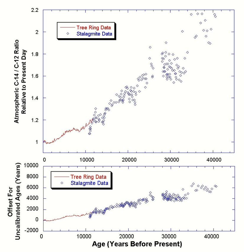
What does one find in the calibration of carbon-14 against actual ages? If one predicts a carbon-14 age
assuming that the ratio of carbon-14 to carbon-12 in the air has stayed constant, there is a slight error
because this ratio has changed slightly. Figure 9 shows that the carbon-14 fraction in the air has decreased
over the last 40,000 years by about a factor of two. This is attributed to a strengthening of the Earth’s
magnetic field during this time. A stronger magnetic field shields the upper atmosphere better from
charged cosmic rays, resulting in less carbon-14 production now than in the past. (Changes in the Earth’s
magnetic field are well documented. Complete reversals of the north and south magnetic poles have
occurred many times over geologic history.) A small amount of data beyond 40,000 years (not shown in
Fig. 9) suggests that this trend reversed between 40,000 and 50,000 years, with lower carbon-14 to
carbon-12 ratios farther back in time, but these data need to be confirmed.
What change does this have on
uncalibrated carbon-14 ages?
The bottom panel of Figure 9
shows the amount of offset in
the uncalibrated ages. The
offset is generally less than
1500 years over the last 10,000
years, but grows to about
6,000 years at 40,000 years
before present. Uncalibrated
radiocarbon ages under-
estimate the actual ages. Note
that a factor of two difference
in the atmospheric carbon-14
ratio, as shown in the top panel
of Figure 9, does not translate
to a factor of two offset in the
age. Rather, the offset is equal
to one half-life, or 5,700 years
for carbon-14. This is only
about 15% of the age of
samples at 40,000 years. The
initial portion of the calibration
curve in Figure 9 has been
widely available and well
Figure 9. Ratio of atmospheric carbon-14 to carbon-12, relative to the present- accepted for some time, so
day value (top panel). Unlike long-term radiometric dating methods, radiocarbon reported radiocarbon dates for
relies on knowing the fraction of radioactive carbon-14 in the atmosphere at the ages up to 11,800 years
time the object being dated was alive. The production of carbon-14 by cosmic generally give the calibrated
rays was up to a factor of about two higher than at present in the timescales over
ages unless otherwise stated.
which radiocarbon can be used. Data for the last 11,800 years comes from tree-
ring counting, while the data beyond that age comes from other sources, such as The calibration curve over the
from a carbonate stalagmite for the data shown here. The bottom panel shows the portions extending to 40,000
offset in uncalibrated ages caused by this change in atmospheric composition. years is relatively recent, but
Tree-ring data are from Stuiver et al., Radiocarbon 40, 1041-1083, 1998; should become widely adopted
stalactite data are from Beck et al., Science 292, 2453-2458, 2001. as well.
14Radiometric Dating of Geologically Young Samples (
concentrations in the water). This allows the dating of these materials by their lack of thorium. A
brand-new coral reef will have essentially no thorium-230. As it ages, some of its uranium decays to
thorium-230. While the thorium-230 itself is radioactive, this can be corrected for. The equations are
more complex than for the simple systems described earlier, but the uranium-234 / thorium-230
                                        method has been used to date corals now for several decades.
                                        Comparison of uranium-234 ages with ages obtained by
                                        counting annual growth bands of corals proves that the
                                        technique is highly accurate when properly used (Edwards et
                                        al., Earth Planet. Sci. Lett. 90, 371, 1988). The method has
                                        also been used to date stalactites and stalagmites from caves,
                                        already mentioned in connection with long-term calibration of
                                        the radiocarbon method. In fact, tens of thousands of uranium-
                                        series dates have been performed on cave formations around
                                        the world.

The uranium-234 / thorium-230 method is now being used to date animal and human bones and teeth.
Previously, dating of anthropology sites had to rely on dating of geologic layers above and below the
artifacts. But with improvements in this method, it is becoming possible to date the human and animal
remains themselves. Work to date shows that dating of tooth enamel can be quite reliable. However,
dating of bones can be more problematic, as bones are more susceptible to contamination by the
surrounding soils. As with all dating, the agreement of two or more methods is highly recommended
for confirmation of a measurement. If the samples are beyond the range of radiocarbon (e.g., > 40,000
years), a second method for confirmation of thorium-230 ages may need to be a non-radiometric
method such as ESR or TL, mentioned below.

Non-Radiometric Dating Methods for the Past 100,000 Years

We will digress briefly from radiometric dating to talk about other dating techniques. It is important to
understand that a very large number of accurate dates covering the past 100,000 years has been obtained
from many other methods besides radiometric dating. We have already mentioned dendrochronology (tree
ring dating) above. Dendrochronology is only the tip of the iceberg in terms of non-radiometric dating
methods. Here we will look briefly at some other non-radiometric dating techniques.

Ice Cores. One of the best ways to measure farther back in time than tree rings is by using the seasonal
variations in polar ice from Greenland and Antarctica. There are a number of differences between snow
layers made in winter and those made in spring, summer, and fall. These seasonal layers can be counted
just like tree rings. The seasonal differences consist of a) visual differences caused by increased bubbles
and larger crystal size from summer ice compared to winter ice, b) dust layers deposited each summer, c)
nitric acid concentrations, measured by electrical conductivity of the ice, d) chemistry of contaminants in
the ice, and e) seasonal variations in the relative amounts of heavy hydrogen (deuterium) and heavy
oxygen (oxygen-18) in the ice. These isotope ratios are sensitive to the temperature at the time they fell as
snow from the clouds. The heavy isotope is lower in abundance during the colder winter snows than it is
in snow falling in spring and summer. So the yearly layers of ice can be tracked by each of these five
different indicators, similar to growth rings on trees. The different types of layers are summarized in Table
III.

                                                     16
Ice cores are obtained by drilling very deep holes in the ice caps on Greenland and Antarctica with
specialized drilling rigs. As the rigs drill down, the drill bits cut around a portion of the ice, capturing a
long undisturbed “core” in the process. These cores are carefully brought back to the surface in sections,
where they are catalogued, and taken to research laboratories under refrigeration. A very large amount of
work has been done on several deep ice cores up to 9,000 feet in depth. Several hundred thousand
measurements are sometimes made for a single technique on a single ice core.
A continuous count of layers exists back as far as 160,000 years. In addition to yearly layering, individual
strong events (such as large-scale volcanic eruptions) can be observed and correlated between ice cores. A
number of historical eruptions as far back as Vesuvius nearly 2,000 years ago serve as benchmarks with
which to determine the accuracy of the yearly layers as far down as around 500 meters. As one goes
further down in the ice core, the ice becomes more compacted than near the surface, and individual yearly
layers are slightly more difficult to observe. For this reason, there is some uncertainty as one goes back
towards 100,000 years. Ages of 40,000 years or less are estimated to be off by 2% at most. Ages of 60,000
years may be off by up to 10%, and the uncertainty rises to 20% for ages of 110,000 years based on direct
counting of layers (D. Meese et al., J. Geophys. Res. 102, 26,411, 1997). Recently, absolute ages have
been determined to 75,000 years for at least one location using cosmogenic radionuclides chlorine-36 and
beryllium-10 (G. Wagner et al., Earth Planet. Sci. Lett. 193, 515, 2001). These agree with the ice flow
models and the yearly layer counts. Note that there is no indication anywhere that these ice caps were ever
covered by a large body of water, as some people with young-Earth views would expect.
Table III Polar ice core layers, counting back yearly layers, consist of the following:
Visual Layers Summer ice has more bubbles and larger Observed to 60,000
crystal sizes years ago
Dust Layers Measured by laser light scattering; most Observed to 160,000
dust is deposited during spring and summer years ago
Layering of Elec- Nitric acid from the stratosphere is Observed through
trical Conductivity deposited in the springtime, and causes a 60,000 years ago
yearly layer in electrical conductivity
measurement
Contaminant Soot from summer forest fires, chemistry of Observed through
Chemistry Layers dust, occasional volcanic ash 2,000 years; some
older eruptions noted
Hydrogen and Indicates temperature of precipitation. Yearly layers observed
Oxygen Isotope Heavy isotopes (oxygen-18 and deuterium) through 1,100 years;
Layering are depleted more in winter. Trends observed much
farther back in time
Varves. Another layering technique uses seasonal variations in sedimentary layers deposited underwater.
The two requirements for varves to be useful in dating are 1) that sediments vary in character through the
seasons to produce a visible yearly pattern, and 2) that the lake bottom not be disturbed after the layers are
deposited. These conditions are most often met in small, relatively deep lakes at mid to high latitudes.
Shallower lakes typically experience an overturn in which the warmer water sinks to the bottom as winter
approaches, but deeper lakes can have persistently thermally stratified (temperature-layered) water
masses, leading to less turbulence, and better conditions for varve layers. Varves can be harvested by
17You can also read