Application of high-dimensional fuzzy k-means cluster analysis to CALIOP/CALIPSO version 4.1 cloud-aerosol discrimination - Atmos. Meas. Tech
←
→
Page content transcription
If your browser does not render page correctly, please read the page content below
Atmos. Meas. Tech., 12, 2261–2285, 2019
https://doi.org/10.5194/amt-12-2261-2019
© Author(s) 2019. This work is distributed under
the Creative Commons Attribution 4.0 License.

Application of high-dimensional fuzzy k-means cluster analysis to
CALIOP/CALIPSO version 4.1 cloud–aerosol discrimination
Shan Zeng1,2 , Mark Vaughan2 , Zhaoyan Liu2 , Charles Trepte2 , Jayanta Kar1,2 , Ali Omar2 , David Winker2 ,
Patricia Lucker1,2 , Yongxiang Hu2 , Brian Getzewich1,2 , and Melody Avery2
1 Science Systems and Applications, Inc., Hampton, VA 23666, USA
2 NASA   Langley Research Centre, Hampton, VA 23666, USA

Correspondence: Shan Zeng (shan.zeng@ssaihq.com)

Received: 22 May 2018 – Discussion started: 28 June 2018
Revised: 26 February 2019 – Accepted: 19 March 2019 – Published: 12 April 2019

Abstract. This study applies fuzzy k-means (FKM) clus-            and COCA classification uncertainties are only minimally af-
ter analyses to a subset of the parameters reported in the        fected by noise in the CALIPSO measurements, though both
CALIPSO lidar level 2 data products in order to classify the      algorithms can be challenged by especially complex scenes
layers detected as either clouds or aerosols. The results ob-     containing mixtures of discrete layer types. Our analysis re-
tained are used to assess the reliability of the cloud–aerosol    sults show that attenuated backscatter and color ratio are
discrimination (CAD) scores reported in the version 4.1 re-       the driving factors that separate water clouds from aerosols;
lease of the CALIPSO data products. FKM is an unsuper-            backscatter intensity, depolarization, and mid-layer altitude
vised learning algorithm, whereas the CALIPSO operational         are most useful in discriminating between aerosols and ice
CAD algorithm (COCA) takes a highly supervised approach.          clouds; and the joint distribution of backscatter intensity and
Despite these substantial computational and architectural dif-    depolarization ratio is critically important for distinguishing
ferences, our statistical analyses show that the FKM classifi-    ice clouds from water clouds.
cations agree with the COCA classifications for more than
94 % of the cases in the troposphere. This high degree of
similarity is achieved because the lidar-measured signatures
of the majority of the clouds and the aerosols are naturally
distinct, and hence objective methods can independently and       1   Introduction
effectively separate the two classes in most cases. Clas-
sification differences most often occur in complex scenes         The Cloud-Aerosol Lidar and Infrared Pathfinder Satel-
(e.g., evaporating water cloud filaments embedded in dense        lite Observation (CALIPSO) mission has been developed
aerosol) or when observing diffuse features that occur only       through a close and ongoing collaboration between NASA
intermittently (e.g., volcanic ash in the tropical tropopause     Langley Research Center (LaRC) and the French space
layer). The two methods examined in this study establish          agency, Centre National D’Études Spatiales (CNES) (Winker
overall classification correctness boundaries due to their dif-   et al., 2010). This mission provides unique measurements
fering algorithm uncertainties. In addition to comparing the      to improve our understanding of global radiative effects
outputs from the two algorithms, analysis of sampling, data       of clouds and aerosols in the Earth’s climate system. The
training, performance measurements, fuzzy linear discrim-         CALIPSO satellite was launched in April 2006, as a part
inants, defuzzification, error propagation, and key parame-       of the A-Train constellation (Stephens et al., 2018). The
ters in feature type discrimination with the FKM method           availability of continuous, vertically resolved measurements
are further discussed in order to better understand the util-     of the Earth’s atmosphere at a global scale leads to great
ity and limits of the application of clustering algorithms to     improvements in understanding both atmospheric observa-
space lidar measurements. In general, we find that both FKM       tions and climate models (Konsta et al., 2013; Chepfer et al.,
                                                                  2008).

Published by Copernicus Publications on behalf of the European Geosciences Union.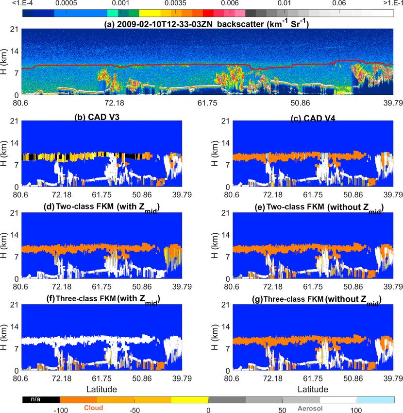
2262                                          S. Zeng et al.: Application of high-dimensional fuzzy k-means cluster analysis

   The Cloud-Aerosol Lidar with Orthogonal Polarization            dimensional probability density functions (PDFs) to dis-
(CALIOP), aboard CALIPSO, is the first satellite-borne             tinguish between clouds and aerosols (Liu et al., 2004,
polarization-sensitive lidar that specifically measures the ver-   2009, 2019). Using a larger number of layer attributes (i.e.,
tical distribution of clouds and aerosols along with their         higher-dimension PDFs) generally yields increasingly accu-
optical and geometrical properties. The level 1 CALIOP             rate cloud and aerosol discrimination. While both V3 and V4
data products report vertically resolved total atmospheric         COCA algorithms use the same five attributes to derive their
backscatter intensity at both 532 and 1064 nm, and the com-        classifications, substantial improvements have been made in
ponent of the 532 nm backscatter that is polarized perpen-         V4 due to much improved calibration, especially at 1064 nm
dicular to the laser polarization plane. The level 2 cloud and     (Liu et al., 2019; Vaughan et al., 2019). The V4 PDFs have
aerosol products are retrieved from the level 1 data and sepa-     been rebuilt to better discriminate dense dust over the Tak-
rately stored into two different file types: the cloud, aerosol,   lamakan Desert, lofted dust over Siberia and the American
and merged layer product files (CLay, ALay, and MLay, re-          Arctic regions, and high-altitude smoke and volcanic aerosol.
spectively) and the cloud and aerosol profile product files        Also, the application of the V4 PDFs has been extended,
(CPro and APro). The profile data are generated at 5 km hor-       and they are now used to discriminate between clouds and
izontal resolution for both clouds and aerosols, with vertical     aerosols in the stratosphere and to features detected at single-
resolutions of 60 m from − 0.5 to 20.2 km, and 180 m from          shot resolution (333 m) in the mid-to-lower troposphere.
20.2 to 30 km. The layer data are generated at 5 km horizon-          CALIPSO has been delivering separate cloud and aerosol
tal resolution for aerosols and at three different horizontal      data products throughout its 12+-year lifetime, and the re-
resolutions for clouds (1/3, 1 and 5 km). The layer products       liable segregation of these products clearly depends on the
consist of a sequence of column descriptors (e.g., latitude,       accuracy of the COCA. However, to the best of our knowl-
longitude, time) that provide information about the vertical       edge, no traditional validation study of the CALIOP CAD
column of atmosphere being evaluated. Each set of column           results has been published in the peer-reviewed literature.
descriptors is associated with a variable number of layer de-      Traditional validation studies typically compare coincident
scriptors that report the spatial and optical properties of each   measurements of identical phenomena acquired by previ-
layer detected in the column.                                      ously validated and well-established instruments to the mea-
   The CALIOP level 2 processing system is composed of             surements acquired by the instrument being validated. For
three modules, which have the general functions of detect-         example, radiometric calibration of the CALIOP attenuated
ing layers, classifying the layers, and performing extinc-         backscatter profiles have been extensively validated using
tion retrievals. These three modules are the selective iter-       ground-based Raman lidars (Mamouri et al., 2009; Mona
ated boundary locator (SIBYL), the scene classifier algo-          et al., 2009) and airborne high spectral resolution lidars
rithm (SCA), and the hybrid extinction retrieval algorithm         (HSRL) (Kar et al., 2018; Getzewich et al., 2018). Further-
(HERA) (Winker et al., 2009). The level 2 lidar processing         more, CALIOP level 2 products have also been thoroughly
begins with the SIBYL module that operates on a sequence of        validated: cirrus cloud heights and extinction coefficients
scenes consisting of segments of level 1 data covering 80 km       have been validated using measurements by Raman lidars
in along-track distance. The module averages these profiles        (Thorsen et al., 2011), Cloud Physics Lidar (CPL) measure-
to horizontal resolutions of 5, 20, and 80 km, respectively,       ments (Yorks et., 2011; Hlavka et al., 2012), and in situ
and detects features at each of these resolutions. Those fea-      observations (Mioche et al., 2010); CALIOP aerosol typ-
tures detected at 5 km are further inspected to determine if       ing has been assessed by HSRL measurements (Burton et
they can also be detected at finer spatial scales (Vaughan et      al., 2013) and Aerosol Robotic Network (AERONET) re-
al., 2009). The SCA is composed of three main submodules:          trievals (Mielonen et al., 2009); and CALIOP aerosol optical
the cloud and aerosol discrimination (CAD) algorithm (Liu          depth estimates have been validated using HSRL measure-
et al., 2004, 2009, 2019), the aerosol subtyping algorithm         ments (Rogers et al., 2014), Raman measurements (Tesche et
(Omar et al., 2009; Kim et al., 2018), and the cloud ice–water     al., 2013), AERONET measurements (Schuster et al., 2012;
phase discrimination algorithm (Hu et al., 2009; Avery et al.,     Omar et al., 2013), and Moderate Resolution Imaging Spec-
2019). Profiles of particulate (i.e., cloud or aerosol) extinc-    troradiometer (MODIS) retrievals (Redemann et al., 2012).
tion and backscatter coefficients and estimates of layer op-       These level 2 validation studies implicitly depend on the as-
tical depths are retrieved for all feature types by the HERA       sumption that the COCA classifications are essentially cor-
module.                                                            rect; however, this fundamental assumption has yet to be ver-
   Clouds and aerosols modulate the Earth’s radiation bal-         ified. This paper is, therefore, a first step in an ongoing pro-
ance in different ways, depending on their composition and         cess of verifying and validating the outputs of the CALIOP
spatial and temporal distributions, and thus being able to         operational CAD algorithm. But unlike traditional validation
accurately discriminate between them using global satellite        studies in which coincident measurements are compared, this
measurements is critical for better understanding trends in        study will compare the outputs of two wholly different clas-
global climate change (Trenberth et al., 2009). The CALIOP         sification schemes applied to the same measured input data.
operational CAD algorithm (COCA) uses a family of multi-           Clearly, one of these two schemes is COCA. The other is the

Atmos. Meas. Tech., 12, 2261–2285, 2019                                              www.atmos-meas-tech.net/12/2261/2019/
S. Zeng et al.: Application of high-dimensional fuzzy k-means cluster analysis                                                                       2263

venerable fuzzy k-means (FKM) clustering algorithm, which           2   CALIOP CAD PDF construction
has a long history of use in classifying features found in satel-
lite imagery (Harr and Elsberry, 1995; Metternicht, 1999;           The CALIOP operational CAD algorithm uses manually
Burrough et al., 2001; Olthof and Latifovic, 2007; Jabari and       derived, multi-dimensional PDFs together with a statisti-
Zhang, 2013).                                                       cal discrimination function to distinguish between clouds
   The rationale for comparing algorithm outputs rather than        and aerosols. Given a standard set of lidar measurements
measurements is twofold. First, no suitable set of coincident       (X1 , X2 , . . . Xm ), separate multi-dimensional PDFs are con-
observations is currently available for use in a global-scale       structed for clouds (P cloud (X1 , X2 , . . . Xm )) and aerosols
validation study. The spatial and temporal coincidence of           (P aerosol (X1 , X2 , . . . Xm )). Discrimination between clouds
ground-based and airborne measurements is extremely lim-            and aerosols for previously unclassified layers is then deter-
ited, and thus any validation exercise would require assump-        mined using
tions about the compositional persistence of features being
                                                                    f (X1 , X2 , . . ., Xm )
compared. (Paradoxically, these are precisely the sorts of as-
                                                                            P cloud (X1 , X2 , . . ., Xm ) − P aerosol (X1 , X2 , . . ., Xm ) k
sumptions that should be obviated by well-designed valida-              =                                                                       ..    (1)
                                                                            P cloud (X1 , X2 , . . ., Xm ) + P aerosol (X1 , X2 , . . ., Xm ) k
tion studies.) Coincident A-Train measurements can be used
in simple cases (Stubenrauch et al., 2013) but have little to       The function f is a normalized differential probability, with
offer in the complex scenes where clouds and aerosols in-           values that range between −1 and 1, and k is a scaling fac-
termingle; e.g., passive sensors cannot provide comparative         tor that is related to the ratio of the numbers of aerosol lay-
information in multi-layer scenes or at cloud–aerosol bound-        ers and cloud layers used to develop the PDFs (Liu et al.,
aries, and the CloudSat radar is only sensitive to large par-       2009, 2019). Within the CALIOP level 2 data products, a per-
ticles and thus cannot help to distinguish between scatter-         centile (integer) value of 100×f , ranging from −100 to 100,
ing targets that it cannot detect (e.g., lofted dust and thin       is reported as the “CAD score” characterizing each feature.
cirrus). Second, COCA is a highly supervised classification         Aerosol CAD scores range from −100 to 0, and cloud CAD
scheme whose decision-making prowess depends on human-              scores range from 0 to 100. Because the nature of clouds is
specified PDFs. FKM, on the other hand, is an unsupervised          quite different from aerosols, most clouds and aerosols can
learning algorithm that, after suitable training, delivers clas-    be distinguished unambiguously. Transition regions where
sifications based on the inherent structure found in the data.      clouds are embedded in aerosols, volcanic ash injected into
The results obtained from the two different algorithms will         the upper troposphere, and optically thick, strongly scatter-
help us better understand global cloud and aerosol distribu-        ing aerosols at relatively high altitudes (e.g., haboobs) can
tions, which is important for all the users of space lidar (e.g.,   still present significant discrimination challenges, but these
atmospheric scientists, weather and climate modelers, instru-       cases occur relatively infrequently.
ment developers). The flexibility of the FKM approach can              The initial version of COCA used only three layer at-
help determine which individual parameters are most influ-          tributes: layer mean attenuated backscatter at 532 nm, hβ532 0 i,

ential in discriminating clouds from aerosols and help eval-        layer-integrated attenuated backscatter color ratio, χ 0 =
uate the degree of improvement to be expected if/when new              0        0 i, and mid-layer altitude, z
                                                                    hβ1064 i/hβ532                              mid . Since then, the
observational dimensions are added to the COCA PDFs.                algorithm has been incrementally improved, and beginning
   Our paper is structured as follows. Section 2 briefly re-        in V3 the COCA PDFs were expanded to five dimensions
views the fundamentals of the COCA PDFs and their appli-            (5-D) by adding layer-integrated 532 nm volume depolariza-
cation to the CALIOP measurements. Section 3 provides an            tion, δv , and the latitude of the horizontal midpoint of the
overview of the FKM algorithm and describes how we have             layer (Liu et al., 2019). Within the CALIPSO analysis soft-
adapted it for use in the CALIOP cloud–aerosol discrimi-            ware, these PDFs are implemented as 5-D arrays that func-
nation task. Section 4 compares the FKM classifications to          tion as look-up tables. However, while the V3 and V4 al-
the V3 and V4 COCA results. These comparisons, which are            gorithms both use five independent measurements, the nu-
made for both individual cases and statistical aggregates, are      merical values in the underlying PDFs are significantly dif-
designed to assess the accuracy of the COCA algorithm in            ferent. The V3 PDFs were rendered obsolete by extensive
general and to quantify changes in performance that can be          changes to the V4 calibration algorithms (Kar et al., 2018;
attributed to the algorithm refinements incorporated in V4          Getzewich et al., 2018; Vaughan et al., 2019) that required
(Liu et al., 2019). Various FKM performance metrics are de-         revising a number of the hβ5320 i probabilities and a global re-

scribed in Sect. 5, including error propagation, key parame-        calculation of the color ratio probabilities. As a result, the V4
ter analysis, fuzzy discriminant analysis and principle com-        CAD algorithm can now be applied in the stratosphere and
ponent analysis. Conclusions and perspectives are given in          to layers detected at single-shot resolution and has greatly
Sect. 6.                                                            improved performance when identifying dense dust over the
                                                                    Taklamakan Desert, lofted dust over Siberian and American
                                                                    Arctic regions, and high-altitude aerosols in the upper tropo-
                                                                    sphere and lower stratosphere (Liu et al., 2019).

www.atmos-meas-tech.net/12/2261/2019/                                                        Atmos. Meas. Tech., 12, 2261–2285, 2019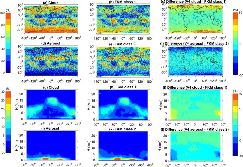
2264                                             S. Zeng et al.: Application of high-dimensional fuzzy k-means cluster analysis

3     Fuzzy k-means cluster analysis                                   the membership matrix, m = 1, an individual i belongs only
                                                                       to a single class j and has a class membership of 0 in all
Cluster analysis is a useful statistical tool to group data into       other classes. Note also that, in the standard (i.e., not fuzzy)
several categories and has been successfully applied to satel-         k-means algorithm, mij can be only 1 or 0 (i.e., a point can
lite observations to discriminate among different features of          only belong to one cluster) but that intermediate values are
interest (Key et al., 1989; Kubat et al., 1998; Omar et al.,           permitted in the FKM method (i.e., a point can partially be-
2005; Zhang et al., 2007; Usman, 2013; Luo et al., 2017;               long to a particular cluster). The sum of the fuzzy member-
Gharibzadeh et al., 2018). There are many different types              ships for an individual over all classes is equal to 1 (Eq. 3),
of clustering methods, such as connectivity-based, centroid-           and there will be at least one individual with some non-zero
based, density-based, and distribution clustering, and these           membership belonging to each class (Eq. 4). These defining
are typically trained using either supervised or unsupervised          relationships are written as
learning techniques. In this paper, we focus on a centroid-
based, unsupervised learning approach known as the fuzzy
k-means (FKM) method. As the name implies, classifica-
                                                                       mij ∈ [0, 1] , i = 1. . .n, j = 1. . .k                       (2)
tion ambiguities are expressed in terms of fuzzy logic (i.e.,
                                                                       k
as opposed to “crisp”/binary logic), and thus every point              X
processed by the clustering algorithm is assigned some de-                    mij = 1, i = 1. . .n, and                              (3)
                                                                       j =1
gree of membership in all categories, rather than belonging
                                                                         n
solely to just one category. FKM membership values range               X
                                                                              mij > 0, j = 1. . .k.                                  (4)
from 0 to 1 and thus are comparable to the operational CAD             i=1
scores. In addition, the shapes and density distributions of
multi-dimensional observations of clouds and aerosols from
lidar are well suited for the centroid-based clustering tech-
                                                                       To determine the best solution, based on minimization of the
nique used by the FKM classification method. With the ex-
                                                                       WCSS, a classic objective function, J , is built so that the best
ception of latitude, our FKM implementation uses the same
                            0 i, χ 0 , δ , and z                       solution is the one that minimizes J (Bezdek, 1981, 1984;
inputs as COCA; i.e., hβ532             v       mid . We make this
                                                                       McBratney and Moore, 1985). The functional form of J is
choice because clouds and aerosols show distinct centers in
       0 i, δ , χ 0 , z
the hβ532     v        mid attribute space, whereas adding lat-
itude degrades the separation between cluster centers and
adds significantly to class overlap. A key parameter analysis                           k
                                                                                      n X
                                                                                                  φ
                                                                                      X
                                                                                                 mij dij2 xil , cj l ,

(described in Sect. 5) demonstrates that latitude does not pro-        J (M, C) =                                                    (5)
vide intrinsic information that helps to distinguish between                          i=1 j =1

aerosols and cloud, nor does it improve the reliability of the
cluster membership values (e.g., Wilks’ lambda, a measure
of the difference between classes also introduced in Sect. 5.,         where C (cj l ; j = 1, . . . , k; l = 1, . . . , p) is a matrix of
deteriorates from ∼ 0.2 to ∼ 0.5). However, for probabilistic          class centers, and d 2 (xil , cj l ) is the squared distance be-
systems (e.g., COCA), latitude can be useful, simply because           tween individual xil and class center cj l according to a cho-
some feature types are more likely than others to occur within         sen definition of distance (e.g., the Mahalanobis distance; see
specific latitude–altitude bands (e.g., at altitudes of 9–11 km,       Sect. 2.3). The objective function is the squared error from
significant aerosol loading is much more likely at 45◦ N than          class centers weighted by the φth power (fuzzy weighting
at 60◦ S).                                                             exponent) of the membership values. For the least meaning-
                                                                       ful value, φ = 1, J minimizes only at crisp partitions (the
3.1    FKM algorithm architecture                                      memberships converge to either 0 or 1), with no overlap be-
                                                                       tween cluster boundaries. Increasing the value of φ tends
Given a set of observations X = (X1 , X2 , . . . , Xn ), where         to degrade memberships towards fuzzier states where there
each observation is a p-dimensional real vector, FKM log-              are more overlaps between the boundaries of clusters. For a
ical clustering aims to partition the n observations into k            specified value of φ, minimization of objective function J
(≤ n) sets S = {S1 , S2 , . . ., Sk } so as to “minimize the within-   optimizes the solutions for the membership matrix M and
cluster sum of squares (WCSS) and maximize the between-                its associated centroid matrix C (Bezdek, 1981; McBratney
cluster sum of squares (BCSS)” (Hartigan and Wang, 1979).              and deGruijter, 1992; Minasny and McBratney, 2002). Class
Points on the edge of a cluster may be in the cluster to have          centers are the averages of the individual samples weighted
a lesser degree than points in the center of the cluster. The          by their class membership values raised to the φth power
clustering results (i.e., fuzzy memberships, organized into a          (Eq. 6). The membership (mij ) of an individual belonging
matrix, M, with elements mij , i = 1. . .n; j = 1. . .k) are as-       to a class is the distance between the individual and the class
signed values between 0 and 1 (Eq. 2). When elements of                center divided by the sum of the distances between the indi-

Atmos. Meas. Tech., 12, 2261–2285, 2019                                                     www.atmos-meas-tech.net/12/2261/2019/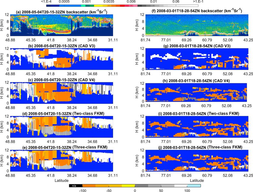
S. Zeng et al.: Application of high-dimensional fuzzy k-means cluster analysis                                                         2265

                                                                             Before running the FKM code (from Minasny and
                                                                          McBratney, 2002), we prepared our data by sampling, train-
                                                                          ing, and filtering (Sect. 2.1 and 2.2). We also selected a rea-
                                                                          sonable method to calculate the distance between individu-
                                                                          als and centers (Sect. 2.3) and determined optimal values for
                                                                          class number and fuzzy exponent (Sect. 2.4). Note the FKM
                                                                          method is directly applied to data to get membership instead
                                                                          of building PDF as in operational algorithm.

                                                                          3.2   Data sample and training

                                                                          As mentioned above, four level 2 parameters are used for
                                                                          our cluster analysis: layer mean attenuated backscatter at
                                                                          532 nm, hβ5320 i, layer-integrated volume depolarization ratio

                                                                          at 532 nm, δv , total attenuated backscatter color ratio, χ 0 , and
                                                                          mid-layer altitude, zmid . The selection of four dimensions is
                                                                          based on many previous studies (e.g., Liu et al., 2004, 2009;
                                                                          Hu et al., 2009; Omar et al., 2009; Burton et al., 2013), which
                                                                          show that clouds, aerosols, and their subtypes are quite dif-
Figure 1. Flowchart illustrating the operation of the fuzzy k-means                                               0 i, δ , and χ 0 are the
                                                                          ferent based on these observations. hβ532      v
algorithm.                                                                fundamental lidar-derived optical properties that form the ba-
                                                                          sis for our discrimination scheme. We also include altitude,
                                                                          as the joint distributions of altitude with the various lidar-
vidual and the centers of all classes (Eq. 7), or                         derived optical properties have proven to be highly effective
                                                                          in identifying different feature types.
         n
         P      φ                                                            In this study, we apply FKM at a global scale. For any
             mij xij                                                      given region, results derived from a localized cluster anal-
         j =1
cj l =      n           , j = 1, 2. . .k, l = 1, 2. . .p,           (6)   ysis will likely give us better classifications compared to
            P       φ                                                     the results from a global-scale analysis, but investigating
                mij
           i=1                                                            and/or characterizing these differences lies well beyond the
             −2/(φ−1)                                                     scope of this study. The data sample size also strongly in-
            dij
mj l =                   ,    i = 1, 2. . .n, j = 1, 2. . .k, and   (7)   fluences the clustering results. For example, clustering into
           k
          P     −2/(φ−1)                                                  two classes with a full complement of CALIPSO data could
              dij
         j =1                                                             identify clear and “not clear” scenes. If clear scenes are ex-
                                                                          cluded, clustering could separate clouds and aerosols. If only
To obtain centroid (Eq. 6) and membership (Eq. 7) solutions,              clear scenes are included, clustering could possibly provide
Picard iterations (Bezdek et al., 1984) are applied until the             a means of identifying different surface types. With only
centers or memberships are constant to within some small                  cloudy data, clustering could be used to derive thermody-
value (see the algorithm flowchart in Fig. 1). We first ini-              namic phase classification. With only aerosol data, cluster-
tialize the memberships as random values using a uniform                  ing is actually aerosol subtyping. With only liquid cloud data,
distribution that satisfies all conditions given by Eqs. (2),             clustering could separate cumulus and stratocumulus. So, the
(3) and (4). We then calculate class centers and recalculate              size and composition of the dataset is very important for our
memberships according to the new centers. If the new mem-                 analysis, which strongly depends on the objective of the clas-
berships do not change compared to the old ones (or change                sification.
only within a small difference ε), the clustering process ends.              To extrapolate the classification of identifiable elements
Otherwise, we recalculate the new centers and new member-                 using FKM from a small subset to a broader population,
ships. If the algorithm does not converge after a fixed number            we identify an appropriate training dataset from which the
of iterations, the procedure is reinitiated using newly (and              classifications can be derived (Burrough et al., 2000). This
again randomly) specified initial cluster centers. This pro-              training data should be representative of the broader sample
cess repeats until the algorithm converges to a point where               for which the classification will be implemented (i.e., both
the relative change in the objective function (calculated from            must span similar domains). To ensure the selection of an
Eq. 5, which quantifies the changes in both the memberships               appropriate training dataset, the shapes of the PDFs of the
and centers) is less than ε (0.001) and saves the best mem-               relevant parameters derived from any proposed training set
berships and centers that result from the optimum random                  should closely match the shapes of the corresponding param-
initiation corresponding to the least objective function.                 eter PDFs derived from the global long-term dataset. Data

www.atmos-meas-tech.net/12/2261/2019/                                                        Atmos. Meas. Tech., 12, 2261–2285, 2019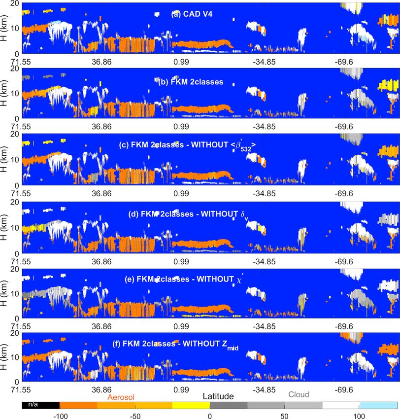
2266                                               S. Zeng et al.: Application of high-dimensional fuzzy k-means cluster analysis

Table 1. Filter thresholds for FKM lidar observables.                  et al. (2003), we should apply the Euclidean distance to un-
                                                                       correlated variables on the same scale when attributes are
       Lidar observable          Filter criteria                       independent and the clusters are spherically shaped clouds.
       Mean attenuated                  0 i ≤ 0.2 sr−1 km−1
                                 0 ≤ h β532                            The diagonal distance is also insensitive to statistically de-
       backscatter at 532 nm                                           pendent variables but clusters are not required to have spher-
       Integrated volume         0 ≤ δv ≤ 2                            ically shaped clouds. The Mahalanobis distance can be used
       depolarization ratio                                            for correlated variables on the same or different scales and
       Total attenuated          0 ≤ χ0 ≤ 2                            when the clusters are ellipsoid-shaped clouds. The Maha-
       backscatter color ratio                                         lanobis distance (dij ) of an observation i from a set of ob-
                                                                       servations (xil ) with centers cj l (xil -cj l is an l-dimensional
                                                                       vector) is defined in Eq. (8) (Mahalanobis, 1936):
from the month of January 2008 are used to determine the op-                               T
                                                                       dij2 = xil − cj l        S−1 xil − cj l , i = 1, 2. . .n,

timal number of classes (k) and fuzzy exponent (φ) required
for classification and optimal values of the performance pa-              j = 1, 2. . .k, l = 1, 2. . .p.                            (8)
rameters, and to calculate class centroids for interpretation of
similarities and differences between classes. To avoid errors          S−1 (an l × l matrix) is the inverse of the covariance ma-
due to small sample sizes, we used the same month of global            trix of the observations. Note superscript T indicates that the
observations (January 2008) to do the subsequent compar-               vector should be transposed. If the covariance matrix is a di-
isons with COCA results.                                               agonal matrix, the Mahalanobis distance calculation returns
   Figure 2 shows approximate probability density functions            the normalized Euclidean distance. In this work, we use the
(computed by normalizing the sum of the occurrence fre-                Mahalanobis distance specifically because the three lidar ob-
quencies to 1) for different lidar observables for liquid wa-          servables used both in FKM and COCA are not independent.
ter clouds, ice clouds composed of either randomly or hori-            Each is a sum (or mean) of the measured backscatter sig-
zontally oriented ice crystals, and aerosols during all of Jan-        nal over some altitude range, with the relationships between
uary 2008. Liquid water clouds have the largest hβ532 0 i and χ 0      them given as follows:
values compared with other species. Aerosols generally have
                              0 i, and ice clouds have the largest                     N
the smallest χ 0 , δv , and hβ532                                        0          1 X
                                                                        β532 =           β0              0
                                                                                                (zn ) + β532,⊥ (zn ) ,              (9a)
δv compared with the other two species. There is overlap be-                        N n=1 532,k
tween species, but these three parameters are still sufficient                N
to separate aerosols and different phases of cloud in most                           0
                                                                              P
                                                                                    β532,⊥ (zn )
cases. Figure 2d, e, and f are from a single half orbit (2008-                n=1
                                                                       δv =                         ,                               (9b)
09-06T01-35-29ZN) of observations. The PDFs of one half                        N
                                                                               P     0
orbit and 1 month of observations appear to agree very well,                        β532,k (zn )
                                                                              n=1
which means that focused feature clustering studies that use                                        N
the FKM method can be applied to a small sample such as                                             P      0
                                                                                                          β1064 (zn )
                                                                                       0
                                                                                     β1064
one-half orbit of observations and not cause significant bi-                                        n=1
                                                                       and χ 0 =        0 i     =                       .           (9c)
ases to the standard full dataset.                                                   hβ532           N
                                                                                                     P     0 (z )
                                                                                                          β532 n
                                                                                                    n=1
3.3    Data filtering
                                                                       In these expressions, the subscripts k and ⊥ represent contri-
We filtered the training data to eliminate outliers in the             butions from the 532 nm parallel and perpendicular channels,
   0 i, δ , and χ 0 measurements that were physically un-
hβ532     v                                                            respectively. Note in particular that the signals measured in
realistic (i.e., either too high or too low). Eliminating these        the 532 nm parallel channel contribute to all three quantities.
extreme values speeds up the processing, and the training al-
gorithm converges more rapidly. The selected filter thresh-            3.5    The choice of class k and fuzzy exponent φ
olds retain more than 98 % of all features within the original
dataset. A summary of the thresholds is given in Table 1. The          The selection of an optimal number of classes k (1 < k < n)
selection of these thresholds is based on the PDFs shown in            and degree of fuzziness φ (φ > 1) has been discussed in many
Fig. 2.                                                                previous studies (Bezdek, 1981; Roubens, 1982; McBratney
                                                                       and Moore, 1985; Gorsevski, 2003). The number of classes
3.4    Distance calculation                                            specified should be meaningful in reality and the partition-
                                                                       ing of each class should be stable. For each generated clas-
The distances between attributes can be calculated in dif-             sification, analyses need to be performed to validate the re-
ferent ways (e.g., Euclidean distance, diagonal distance and           sults. Among different validation functions, the fuzzy perfor-
Mahalanobis distance). According to a study by Gorsevski               mance index (FPI) and the modified partition entropy (MPE)

Atmos. Meas. Tech., 12, 2261–2285, 2019                                                         www.atmos-meas-tech.net/12/2261/2019/
S. Zeng et al.: Application of high-dimensional fuzzy k-means cluster analysis                                                           2267

Figure 2. Comparisons of approximate probability density functions computed by normalizing the sum of the occurrence frequencies to 1; the
top row (a–c) shows data from all of January 2008; bottom row (d–f) shows data from a single half orbit (6 September 2008, 01:35:29 GMT).
The left column (a, d) compares total attenuated backscatter PDFs; the center column (b, e) compares volume depolarization ratio PDFs;
and the right column (c, f) compares total attenuated backscatter color ratio PDFs. Black lines represent aerosols, blue lines represent liquid
water clouds, red lines represent ice clouds dominated by horizontal oriented ice (HOI), and magenta lines represent ice clouds dominated
by random oriented ice (ROI).

are considered two of the most useful indices among seven                 maximum of the objective function, where
examined by Roubens (1982) to evaluate the effects of vary-
ing class number. The FPI is defined as in Eq. (10), where                         k×F −1
                                                                          FPI = 1 −          , and                                        (10)
F is the partition coefficient calculated from Eq. (11). The                           k−1
MPE is defined as in Eq. (12), with the entropy function (H )                1X n X  k
calculated from Eq. (13).                                                 F=            m2 ;                                              (11)
                                                                             n i=1 j =1 ij
   The ideal number of continuous and structured classes (k)
can be established by simultaneously minimizing both FPI                          H
                                                                          MPE =        , and                                              (12)
and MPE. For the fuzziness exponent, if the value of φ is                       log k
too low, the classes become more discrete and the member-                       n X  k
                                                                             1X
ship values either approach 0 or 1. But if φ is too high, the             H=            mij × log mij ; and                               (13)
classes will not provide useful discrimination among samples                 n i=1 j =1
and classification calculations may fail to converge. McBrat-                         n X  k
                                                                          ∂J (M, C) X          φ
                                                                                              mij log mij dij2 .

ney and Moore (1985) suggested that the objective function                         =                                                      (14)
(Eq. 14, Bezdek, 1981) decreases with increasing of both                      ∂φ     i=1 j =1
fuzzy exponent (φ) and the number of classes (k). They plot-
ted a series of objective functions versus the fuzzy exponent             Using 1 month of layer optical properties reported in the
(φ) for a given class where the best value of φ for that class            CALIOP level 2 merged layer products, we created Fig. 3
is at the first maximum of objective function curves (Odeh                to determine optimal values for k and φ. From this figure,
et al., 1992a; McBratney and Moore, 1985; Triantafilis et al.,            we conclude that the ideal number classes for CALIOP layer
2003). Therefore, choosing an optimal combination of class                classification is either three or four, with corresponding fuzzy
number (k) and fuzzy exponent (φ) is established on the ba-               exponents equal to 1.4 or 1.6 (we use 1.4 for the analy-
sis of minimizing both values of FPI and MPE and the least                ses in this paper). Before exploring the clustering results to
                                                                          see what each class represents, we can immediately confirm
                                                                          that using three classes would be physically meaningful (i.e.,
                                                                          these three classes may be aerosols, liquid water clouds, and
                                                                          ice clouds). Similarly, two classes could represent aerosols
                                                                          and clouds. In the following study, we will choose k equal to
                                                                          2 or 3 and φ equal to 1.4.

www.atmos-meas-tech.net/12/2261/2019/                                                        Atmos. Meas. Tech., 12, 2261–2285, 2019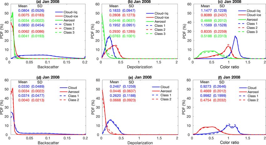
2268                                             S. Zeng et al.: Application of high-dimensional fuzzy k-means cluster analysis

Figure 3. Determination of the number of classes, k, and the fuzzy exponent, φ, for the FKM cloud–aerosol discrimination algorithm: (a) FPI
(y axis) versus class number k (x axis) for different values of fuzzy exponent φ (different colors); (b) MPE (y axis) versus class number k
(x axis) for different values of fuzzy exponent φ (different colors); and (c) objective function values (y axis) versus the fuzzy exponent φ (x
axis) for various class numbers (different colors).

4     Cluster results and comparison with V3 and V4 data                  class CADFKM (Fig. 4c and d) but are correctly classified
                                                                          as clouds by the operational V4 algorithms.
4.1    CAD from the fuzzy k-means algorithm                                  The differences between the FKM and V4 COCA classifi-
                                                                          cations are most prominent for layers detected in the strato-
According to Liu et al. (2009), the CAD score for any layer               sphere (i.e., layers rendered in black in Fig. 4b). In the
is the difference between the probability of being a cloud and            Northern Hemisphere, between 71.55 and 36.86◦ N, a dif-
the probability of being an aerosol (Eq. 15). We calculate the            fuse, weakly scattering layer is intermittently detected at al-
FKM CAD score in a similar way, where the COCA proba-                     titudes between 12 and 18 km. This layer most likely origi-
bilities are replaced with FKM membership values. For the                 nated with the eruption of the Kasatochi volcano on 7 Au-
three-class FKM analyses, the cloud membership value is the               gust 2008 (Krotkov et al., 2010). But while V4 COCA clas-
sum of memberships of ice and water clouds (two classes).                 sifies these layers as aerosols, both FKM methods iden-
The FKM CAD score is found using                                          tify them as clouds. In the Southern Hemisphere, south of
                                                                          69.6◦ S, a faint polar stratospheric layer is detected continu-
              M cloud − M aerosol
CADFKM =                          × 100.                       (15)       ously, with a mean base altitude at ∼ 11 km and a mean top at
              M cloud + M aerosol                                         ∼ 15 km. Once again, the V4 COCA classifies this feature as
Figure 4 compares the operational V3 and V4 CAD products                  a moderate- to high-confidence aerosol layer and the three-
and our CADFKM classifications for a single nighttime orbit               class FKM classifies it as a high-confidence cloud. However,
segment (6 September 2008, beginning at 01:35:29 GMT).                    unlike the Northern Hemisphere case, the two-class FKM
Generally speaking, CADFKM values from both the two-class                 identifies this as low-confidence aerosol. Correctly classify-
and three-class analyses are quite similar to both the V3                 ing stratospheric features that occupy the “twilight zone” be-
and V4 COCA values. When COCA CAD scores are pos-                         tween aerosols and highly tenuous clouds (Koren et al., 2007)
itive (namely clouds, shown in whitish colors in Fig. 4) in               is likely to be difficult for unsupervised learning methods,
V3 and V4, the two-class and three-class CADFKM values                    due to the extensive overlap in the available lidar observables
are also positive. Likewise, when COCA CAD scores are                     for the two classes. Class separation is typically (though not
negative (namely aerosols, yellowish colors in Fig. 4), the               always) more distinct within the troposphere.
two-class and three-class CADFKM values are also negative.
Furthermore, the particular orbit selected here includes the              4.2   Uncertainties: class overlap
observations of a plume of high, dense smoke lofted over
low water clouds (latitudes between 0◦ and 20◦ S, shown                   The confusion index (CI) is a measure of the degree of class
within the red oval in Fig. 4a). For these water clouds be-               overlap or uncertainty between classes (Burrough and Mc-
neath dense smoke, both the V3 operational CAD and the                    Donnell, 1998). In effect, it measures how confidently each
two-class CADFKM label them as clouds with low positive                   individual observation has been classified. CI values are cal-
values. On the other hand, the V4 operational CAD and the                 culated from Eq. (16), where mmax denotes the biggest mem-
three-class CADFKM return higher values much closer to                    bership value and mmax−1 is the second biggest membership
100. The reasons for these differences will be discussed in               value for each individual observation (i):
Sect. 5.2 and 5.4. Note too that weakly scattering edges of
cirrus clouds (hereafter, cirrus fringes) beyond 69.6◦ S are
misclassified as aerosols by both the two-class and three-                CI = 1 − mmaxi − m(max−1)i .                                    (16)

Atmos. Meas. Tech., 12, 2261–2285, 2019                                                       www.atmos-meas-tech.net/12/2261/2019/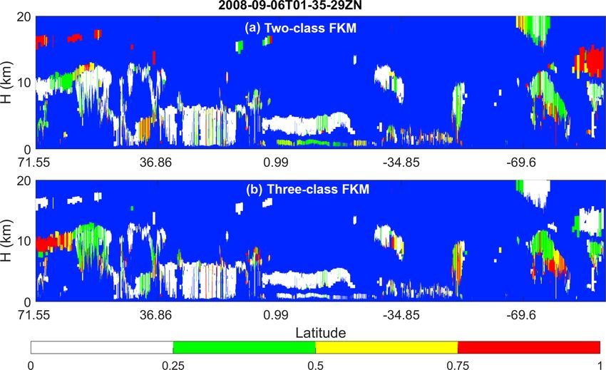
S. Zeng et al.: Application of high-dimensional fuzzy k-means cluster analysis                                                   2269

                                                                       Figure 5. For the same data as shown in Fig. 4; the upper
                                                                       panel (a) shows the confusion index for two-class CADFKM , and
                                                                       the lower panel (b) shows the confusion index for three-class
                                                                       CADFKM . The pure blue color once again indicates those regions
                                                                       where no atmospheric layers were detected.

                                                                       values indicate low-confidence classifications where the ob-
                                                                       servation has roughly equal membership in two classes. For
Figure 4. Nighttime orbit segment from 6 September 2008, begin-        the liquid water clouds beneath dense smoke, the member-
ning at 01:35:29 UTC. The upper panel (a) shows 532 nm atten-          ship values determined by the two-class CADFKM are larger
uated backscatter coefficients. The panels below show the CAD          than 0.5. However, the three-class CADFKM results for these
results as determined by (b) the V3 operational CAD algorithm,         water clouds have low CI values, indicating high-confidence
(c) the V4 operational CAD algorithm, (d) the two-class FKM CAD        classifications into one dominant class, and suggesting that
algorithm, and (e) the three-class FKM CAD algorithm. The red el-
                                                                       the separation between the aerosols and low water clouds is
lipse in the upper panel highlights a dense smoke layer lying above
                                                                       better accomplished when three classes are used. For cloud
an opaque stratus deck. In the CAD images (b–e), stratospheric lay-
ers are shown in black, cirrus fringes are shown in pale blue, and     fringes, the CI values are high for both the two-class and
regions of “clear air” where no features were detected are shown in    three-class CADFKM . According to the CADFKM results, cir-
pure blue. Latitude units are in degrees; positive: north, negative:   rus fringes are somewhat different from the neighboring por-
south.                                                                 tions of the cirrus layer, as they also bear some similarity to
                                                                       the dust particles that are the predominant sources of ice nu-
                                                                       clei (DeMott et al., 2010).
The CI value approaches zero when mmax is much larger than
mmax−1 , indicating that the observation is more likely to be-         4.3   Statistical comparisons of clouds and aerosols
long to one dominant class. CI approaches 1 when mmax is
almost equal to mmax-1 . In such cases, the difference between         In this subsection, we present statistical analyses of our re-
the dominant and subdominant classes is negligible, which              sults for all of January 2008, followed by explorations of in-
creates confusion in the classification of that particular obser-      dividual case studies in the next subsection. We first com-
vation. Note the value (1 – CI) ×100 for the two-class FKM             pare the PDFs of the different lidar-derived optical param-
algorithm is equivalent to the absolute value of the CADFKM            eters used in the two-class and three-class CADFKM classi-
score.                                                                 fications to the PDFs of those same parameters derived for
   Figure 5 shows CI values for two-class and three-class              the COCA classifications (Fig. 6). We also compare the spa-
CADFKM calculated for all layers in the sample orbit. From             tial distribution patterns of the clouds and aerosols identified
the figure, we see that, in most cases, the CI values are low          by FKM and COCA (Fig. 7) and use confusion matrices to
for both the two-class and three-class CADFKM classifica-              quantify the similarity of the corresponding FKM and COCA
tions. The exceptions are stratospheric features (mostly near          classes (Table 2).
polar regions), cloud fringes, high-altitude aerosols, and, for           From Fig. 6, it is evident that the PDFs of hβ532   0 i, δ ,
                                                                                                                                      v
two-class CADFKM only, the liquid water clouds beneath                        0
                                                                       and χ that characterize the clouds and aerosols determined
dense smoke. Low CI values for the CADFKM classifications              by the FKM classifications agree well with the PDFs from
are analogous to high CAD scores assigned by the opera-                the V4 CAD classifications. Figure 6d, e, and f compare
tional CAD algorithm: both indicate high-confidence clas-              the two-class CADFKM results to the operational algorithm.
sifications. Similarly, CADFKM classifications with high CI            In these figures, the PDFs of hβ532 0 i (Fig. 6d), δ (Fig. 6e),
                                                                                                                           v

www.atmos-meas-tech.net/12/2261/2019/                                                    Atmos. Meas. Tech., 12, 2261–2285, 2019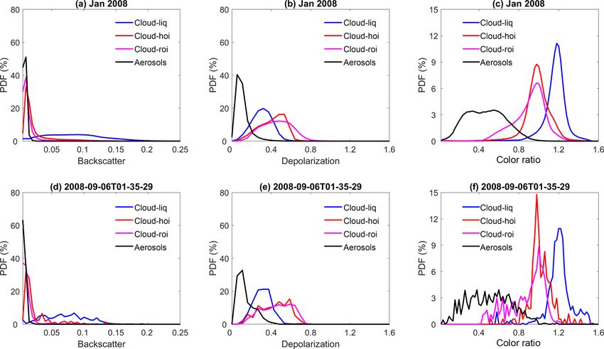
2270                                         S. Zeng et al.: Application of high-dimensional fuzzy k-means cluster analysis

and χ 0 (Fig. 6f) of FKM class 1 (dashed blue lines) agree        ing an unsupervised FKM method is statistically consistent
well with those of V4 cloud PDFs (solid blue lines), while        with the classifications produced by the operational V4 CAD
the PDFs of these different parameters of FKM class 2             algorithm.
(dashed red lines) agree well with those of V4 aerosol               Above, we qualitatively show the operational classification
(solid red lines) PDFs. Figure 6a, b, and c compare the           algorithm agrees well with FKM algorithm. To quantify the
three-class CADFKM results to the operational algorithm.          degree to which the different methods agree with each other,
Once again, the comparisons are quite good: the shapes of         we construct confusion matrices, which use the January 2008
the PDFs of FKM class 1 (dashed blue) agree well with             5 km merged layer data between 60◦ S and 60◦ N to calculate
the V4 water cloud (blue solid) PDFs, while the PDFs of           the concurrent frequency of cloud and aerosol identifications
FKM class 2 (dashed red) and 3 (dashed green) individ-            made by the COCA and CADFKM algorithms. We summa-
ually agree well with, respectively, the V4 ice cloud (red        rize the occurrence frequency statistics in Table 2. From the
solid) and aerosol (green solid) PDFs. The class means for        table, we find that for our test month COCA V3 agrees with
   0 i are smallest for aerosols/class 3 (0.0034 ± 0.0022
hβ532                                                             COCA V4 CAD for 96.6 % of the cases. The agreements are
and 0.0041 ± 0.0193 (km−1 sr−1 ), respectively) and slightly      around 90 % for the entire globe including regions beyond
larger for ice clouds/class 2 (0.0075 ± 0.0086 and 0.0062 ±       60◦ (not shown here). The FKM two-class and three-class
0.0183 (km−1 sr−1 ), respectively). Water clouds/class 1 have     results agree with both V3 and V4 for more than 93 % of the
               0 i mean values (0.0804 ± 0.0526 (km−1 sr−1 )
the largest iβ532                                                 cases. The FKM results agree slightly better with V3 than
and 0.0850 ± 0.0454 (km−1 sr−1 ), respectively). For δv , the     with V4. All algorithms and versions agree on cloud cover-
largest mean values are found for ice clouds/class 2, fol-        age of around 58 % to 66 % of the globe. These values are
lowed by water clouds/class 1 and then aerosol/class 3. Class     well within typical cloud climatology estimates of 50 % to
mean χ 0 is largest for water clouds/class 1 and smallest for     70 % (Stubenrauch et al., 2013). Compared to the two-class
aerosols/class 3. These means and standard deviations are         CADFKM , results from the three-class CADFKM agree some-
also comparable between COCA and FKM classes.                     what better with the classifications from both the V3 and V4
   Figure 7 compares the geographical (panels a–f) and            CAD algorithms. Consistent with previous results in this pa-
zonally averaged (panels g–l) distributions of two-class          per, the three-class CADFKM appears better able to separate
CADFKM occurrence frequencies to the COCA cloud and               clouds and aerosols than the two-class CADFKM . Figure 4
aerosol occurrence frequencies for all data acquired dur-         provides an additional example. For those water clouds be-
ing January 2008. The spatial distributions of clouds and         neath dense smoke, the three-class CADFKM scores are sub-
aerosols are quite different. In January, clouds are mostly lo-   stantially higher than both the two-class CADFKM scores and
cated in the storm tracks, to the east of continents, over the    the operation V3 CAD scores, indicating that the three-class
Intertropical Convergence Zone (ITCZ) and in polar regions.       CADFKM algorithm correctly identifies these features with
Aerosols are more often found over the Sahara, over the sub-      much higher classification confidence. While the discrepan-
tropical oceans, and in south-central and east Asia (Fig. 7a–     cies between the two techniques are pleasingly small, their
f). In the zonal mean plots (Fig. 7g–l), cloud tops are seen      root causes are still of some interest. For example, we note
to extend up to the local tropopause, whereas aerosols are        that the FKM algorithm shows a slight bias toward aerosols
largely confined to the boundary layer. The geographical and      relative to the V4 COCA (a 2.4 % bias for the three-class
vertical distributions of FKM class 1 are quite similar to the    FKM versus a 1.5 % bias for the two-class FKM). At present,
COCA V4 cloud distributions. Likewise, the distributions of       we speculate that the bulk of these differences can be traced
FKM class 2 closely resemble the COCA V4 aerosol distri-          to the dichotomy between supervised (COCA) and unsuper-
butions. Looking at the difference plots (right-hand column       vised (FKM) learning techniques. Given the scope and qual-
of Fig. 7), some fairly large differences are seen in the polar   ity of the data currently available for use by the COCA and
regions, where the composition and intermingling of clouds        FKM methods, the correct classification of layers occupy-
and aerosols are notably different from other regions of the      ing the twilight zone separating clouds and aerosols remains
globe. Many of the layers observed in the polar regions are       somewhat uncertain, and hence different learning strategies
spatially diffuse and optically thin, and thus occupy the mor-    are likely to come to different conclusions, even when pro-
phological twilight zone between clouds and aerosols (Ko-         vided the same evidence. We also calculated the concurrent
ren et al., 2007). Observationally based validation of the fea-   occurrence frequencies for only those features with CI val-
ture types in these regions would likely require extensive in     ues less than 0.75 (or 0.5). When the data are restricted to
situ measurements coincident with CALIPSO observations.           only relatively high-confidence classifications, the FKM re-
Consequently, correctly interpreting the classifications by the   sults agree with V3 and V4 for better than 96 % (or 97 %) of
two algorithms in polar regions based on our knowledge is         the samples tested.
too challenging to draw useful conclusions and lies well be-
yond the scope of this work. Nevertheless, the PDFs and geo-
graphic analyses presented here establish that, excluding the
polar regions, the cloud–aerosol discrimination derived us-

Atmos. Meas. Tech., 12, 2261–2285, 2019                                            www.atmos-meas-tech.net/12/2261/2019/
S. Zeng et al.: Application of high-dimensional fuzzy k-means cluster analysis 2271
Figure 6. PDFs derived from all data from January 2008. The top row compares V4 operational CAD PDFs to the PDFs derived from
CADFKM three-class results. V4 CAD PDFs for liquid water clouds, ice clouds, and aerosols are plotted in, respectively, solid blue, red, and
green lines. Similarly, CADFKM three-class PDFs for classes 1, 2, and 3 are plotted in, respectively, dashed blue, red, and green lines. The
bottom row compares V4 operational CAD PDFs to the PDFs derived from CADFKM two-class results, where once again the V4 CAD PDFs
are shown in solid lines and the CADFKM two-class PDFs are shown in dashed lines. PDFs of hβ532 0 i are shown in the left column (a, d), δ
v
PDFs in the center column (b, e), and χ 0 PDFs in the right column (c, f).
Figure 7. Distributions of feature type occurrence frequencies during January 2008. Panels in the left column show V4 COCA results; panels
in the center column show CADFKM two-class results; and the panels in the right column show the percentages of differences between the
left and center columns. The top two rows show maps of occurrence frequencies as a function of latitude and longitude for clouds (a–c) and
aerosols (d–f). The bottom two rows show the zonal mean occurrence frequencies of clouds (g–i) and aerosols (j–l).
www.atmos-meas-tech.net/12/2261/2019/ Atmos. Meas. Tech., 12, 2261–2285, 20192272 S. Zeng et al.: Application of high-dimensional fuzzy k-means cluster analysis
Table 2. Statistical confusion matrix of a 1-month (January 2008) CAD analysis that shows the agreement percentages (detected as clouds:
C, aerosols: A, or total of clouds and aerosols: T for both algorithms) between different methods (V3: version 3, V4: version 4; FKM: fuzzy
k means).
Agreement (%) V4 FKM (two classes) FKM (three classes)
C A T C A T C A T
V3 C 66.1 2.1 63.8 4.5 64.6 3.7
A 1.2 30.5 1.1 30.6 1.9 29.9
T 96.6 94.4 94.5
V4 C – 59.3 4.9 60.6 3.6
A 1.5 34.4 2.4 33.4
T 93.6 94.0
FKM (two classes) C – – 60.1 0.6
A 2.8 36.5
T 96.7
4.4 Special case studies 1 (also not shown). As seen between ∼ 44 and ∼ 40◦ N, lay-
ers with this combination of layer optical properties are fre-
In this section, we investigate several of the challenging clas- quently misclassified as ice clouds in COCA V3 (Fig. 8b).
sification cases that motivated the extensive changes made However, in COCA V4, these same layers are much more
in COCA in the transition from V3 to V4 (Liu et al., 2019). likely to be correctly classified as aerosol (Fig. 8c). The two-
Comparisons are done for those cases between different al- class and three-class CADFKM classifications both agree with
gorithms and different algorithm versions to see how well COCA V4 for the lofted aerosols but misclassify the dens-
each algorithm or version compares to “the truth” (i.e., as ob- est portions of the dust plume as a low-confidence cloud.
tained by expert judgments). In addition to the dense smoke For the lofted Asian dust case shown in Fig. 8f–j, COCA
over opaque water cloud case shown in Fig. 4, the CADFKM V3 frequently misclassifies dust filaments as clouds, whereas
algorithm, like the operational CAD algorithm, can occasion- COCA V4 correctly identifies the vast majority as dust. (Note
ally have difficulty correctly identifying high-altitude smoke, too that many more layers are detected in V4 as a conse-
dense dust, lofted dust, cirrus fringes, polar stratospheric quence of the changes made to the CALIOP 532 nm calibra-
clouds (PSCs), and stratospheric volcanic ash (Figs. 8–10). tion algorithms (Kar et al., 2018; Getzewich et al., 2018; Liu
We briefly review each of these cases below. et al., 2019).) The two-class and three-class CADFKM clas-
sifications are essentially identical to those determined by
4.4.1 Dust COCA V4 but show higher confidence values for the aerosol
layers.
Two different dust cases are selected for this study (Fig. 8).
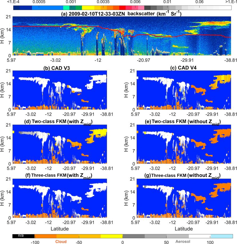
The first case examines nighttime measurements of a deep 4.4.2 High-altitude smoke
and sometimes extremely dense dust plume in the Takla-
makan Desert beginning at 20:15:32 UTC on 4 May 2008, An unprecedented example of high-altitude smoke plumes
as shown in Fig. 8a–e. The second case investigates spatially was observed by CALIPSO during the “Black Saturday” fires
diffuse Asian dust lofted high into the atmosphere while be- that started 7 February 2009, quickly spread across the Aus-
ing transported toward the Arctic during a nighttime orbit tralian state of Victoria, and eventually lofted well into the
segment beginning at 18:28:54 UTC on 1 March 2008, as stratosphere (de Laat et al., 2012). Figure 9 shows extensive
shown in Fig. 8f–j. CAD classifications are color-coded as smoke layers at 10 km and higher on Monday, 10 February,
follows: regions where no features were detected are shown between 20 and 40◦ S. In the V3 CALIOP data products,
in pure blue; V3 stratospheric features are shown in black; stratospheric layers (i.e., layers with base altitudes above
cirrus fringes are shown in pale blue; aerosol-like features are the local tropopause) were not further classified as clouds
shown using an orange-to-yellow spectrum, with orange in- or aerosols but instead were designated as generic “strato-
dicating higher confidence and yellow lower confidence; and spheric features” (Liu et al., 2019). Consequently, COCA V3
cloud-like features are rendered in grayscale, with brighter misclassifies these smoke layers as clouds when their base
and whiter hues indicating higher classification confidence. altitude is below the tropopause and as stratospheric features
Dust layers in the Taklamakan Desert exhibit high (532 nm) when the base altitude is higher (Fig. 9b). On the other hand,
attenuated backscatter coefficients, high depolarization ratios the V4 CAD correctly identifies them as aerosols (Fig. 9c).
(not shown), and attenuated backscatter color ratios close to In analyzing this scene, we used two separate versions of the
Atmos. Meas. Tech., 12, 2261–2285, 2019 www.atmos-meas-tech.net/12/2261/2019/S. Zeng et al.: Application of high-dimensional fuzzy k-means cluster analysis 2273
Figure 8. The top row shows 532 nm attenuated backscatter coefficients for (a) dust in the Taklamakan basin on 4 May 2008 and (f) lofted
Asian dust being transported into the Arctic on 1 March 2008. The rows below show the CAD results reported by four different algorithms:
COCA V3 (b, g), COCA V4 (c, h), the two-class CADFKM (d, i), and the three-class CADFKM (e, j).
FKM algorithm. Our standard configuration used zmid as one 7–8 August 2008 in the central Aleutian Islands. Volcanic
of the classification attributions, while a second, trial con- aerosols remained readily visible in the CALIOP images
figuration omitted zmid . For the two-class FKM, both con- for over 3 months after the eruption (Prata, et al., 2017).
figurations successfully identified the high-altitude smoke as On 5 October 2008, CALIOP observed the “aerosol plume”
aerosol (Fig. 9d and e). But for the three-class FKM, includ- near the tropopause at ∼ 17:30:18 UTC. COCA V3 classi-
ing zmid as a classification attribute introduced uniform mis- fied those layers with base altitudes above the tropopause
classification of the lofted smoke as cloud (Fig. 9f). How- as “stratospheric features” (black regions in Fig. 10b) and
ever, when zmid is omitted, the three-class FKM correctly misclassified a substantial portion of the lower tropospheric
recognizes the smoke as aerosol (Fig. 9g). This is because in- layers as clouds. Those segments that were correctly classi-
cluding altitude information can introduce unwanted classifi- fied as aerosol were frequently assigned low CAD scores. In
cation uncertainties when attempting to distinguish between contrast, COCA V4 and both versions of the CADFKM with
high-altitude clouds and aerosols, both of which are located zmid as inputs show greatly reduced cloud classifications, and
at similar altitudes and have similar optical properties. Alti- the aerosols have high-confidence CAD scores. Again, when
tude is not a driving factor for classifications and adds confu- altitude information is not included, the FKM algorithm pro-
sion in the memberships defined by the Mahalanobis distance duces a better separation of clouds and aerosols at high al-
(see Eqs. 7 and 8) in these particular cases. More details are titudes, for the same reasons as in the high-altitude smoke
given in Sect. 5.1. When high-altitude depolarizing aerosols case.
and ice clouds appear at the same time, either increasing the
number of classes to four or omitting zmid as an input will re-
solve large fractions of the potential misclassifications from 5 Discussion
the FKM method.
Section 5 compares FKM and COCA using statistical anal-
4.4.3 Volcanic ash yses and individual case studies. In this section, we explore
the application of various metrics used to evaluate the quality
Figure 10 shows an example of ash from the Kasatochi vol- of the FKM and COCA classifications. The questions we ad-
cano (52.2◦ N, 175.5◦ W), which erupted unexpectedly on dress are (a) how much improvement can be made by adding
www.atmos-meas-tech.net/12/2261/2019/ Atmos. Meas. Tech., 12, 2261–2285, 2019You can also read