Information: to Harvest, to Have and to Hold * - arXiv

Information: to Harvest, to Have and to Hold *
 Marin van Heel 1,2,3 ** and Michael Schatz 4
 **corresponding author
1
 Brazilian Nanotechnology National Laboratory (LNNano), Brazilian Centre for Research in
Energy and Materials (CNPEM), 13083-970 Campinas, São Paulo, Brazil.
2
 Emeritus Professor, Leiden University, Biology Department (NeCEN), The Netherlands.
3
 Emeritus Professor of Structural Biology, Imperial College London, London, UK.
4
 Image Science Software GmbH, Berlin, Germany.

 Abstract
Signal-to-Noise Ratios (SNRs) and the Shannon-Hartley channel capacity are metrics
that help define the loss of known information while transferring data through a noisy
channel. These metrics cannot be used for quantifying the opposite process: the
harvesting of new information. Correlation functions and correlation coefficients do play
an important role in collecting new information from noisy sources. However, Bershad
and Rockmore [Bershad & Rockmore, 1974] based their correlation-to-SNR formulas on
a priori assumptions in Real-space and in Fourier-space, which cannot be fulfilled
simultaneously. Their formulations were subsequently copied literally to the practical
science of electron microscopy, where those a priori assumptions now distort most
quality metrics in Cryogenic Electron Microscopy (cryo-EM). Cryo-EM became a great
success in recent years [Wiley Award 2017; Nobel prize for Chemistry 2017] and became
the method of choice for revealing structures of biological complexes like ribosomes,
viruses, or corona-virus spikes, vitally important during the current COVID-19 pandemic.
Those early misconceptions, however, now interfere with the objective comparison of
independently obtained results, especially where it concerns local details. We found that
the roots of these problems significantly pre-date those 1970s publications and were
already inherent in the original SNR definitions, introduced more than a century ago. We
here propose novel metrics to assess the amount of information harvested in an
experiment, information which is measured in bits. These new metrics assess the total
amount of information collected on an object, as well as the information density
distribution within that object. The new metrics can be applied everywhere where data is
collected, processed, compressed, or compared. As an example, we compare the
structures of two recently published SARS-CoV-2 spike proteins. We also introduce new
metrics for transducer-quality assessment in many sciences including: cryo-EM,
biomedical imaging, microscopy, signal processing, photography, tomography, etc.

Keywords: SNR, Shannon Information, DQE, FRC, FSC, FRI, FSI, Cryo-EM,
 SARS-CoV-2, Sampling Theorem, Channel Capacity, TIE,
 Transducer Information Efficiency, Degrees of Freedom.

*This paper is dedicated to the memory of Professor James Barber (1940-2020)

 1

I) Introduction

We here discuss the collection of new information on objects present in noisy data. Such
information harvesting has not been properly integrated into information theory. The
Signal-to-Noise Ratio (SNR) and Shannon’s information capacity concepts are focused on
not losing the information contained in a message while transferring that message through a
channel. The channel can be a physical telephone line or an abstract operation like the
storing and retrieving of messages from a computer hard-drive. The very concept of a
mathematical theory of communication [Shannon 1948], implies one knows all information
deterministically at point A that one wants to send through the channel to point B. If there
is no signal entering the channel at A, there is also no way for an observer at B to know from
the arriving noise that it does not contain some hidden signal and that thus the SNR is zero.
The observer needs to have the a priori knowledge that no signal was sent from A.

Collecting new information from a noisy source is an entirely different matter. The signal
enters a transducer in the form of waves which are detected as intensities, and integrated
over a certain time in order to form a measurement (a measurement vector). The integration
time τ is an important concept: when using a very short integration time, the measurement
vectors will be very noisy and the cross-correlation coefficient (CCC) between different
measurement vectors will be small and noisy. What we want to emphasise here is that the
CCC is not an intrinsic property of the source, but rather a property of the measurement.
CCC-based approaches can be used to harvest new information which is not possible with
the SNR-oriented approaches. One can use cross-correlations to search for similarities
between two independent Real-space measurements from the same source. Correlations can
also be used to find multiple copies of signals in noisy measurements. Once identified, one
can compare such signals (or averaged signals) by Real-space CCCs.

The CCCs in Real-space are, however, mostly only of limited use in 2D or 3D data analysis,
due to the typical overwhelming presence of low-frequency components in normal images
[Van Heel 1992]. It makes more sense to study CCCs in Fourier-space as function of spatial
frequency. Fourier-space metrics like the Fourier Ring Correlation (FRC) [Van Heel 1982;
Saxton 1982] and the Fourier Shell Correlation (FSC) [Harauz 1986] are now used routinely
to assess the similarity between two images or two 3D volumes. Originally used primarily
in electron microscopy, they have now proliferated into most fields of scientific imaging
(see: [Baksh 2020; Donnelly 2020; Loetgering 2020]). The CCCs in Fourier-space are
measured over rings in 2D Fourier-space (FRC), or shells in 3D Fourier-space (FSC). The
FRC/FSC cross-correlation coefficients, are neither SNRs nor information in the sense of
Shannon. Their values increase when more data is accumulated, but the question remains:
how to integrate these metrics into the world of SNRs, and Shannon’s information concepts?

To get to the heart of the matter, we will first cover some underlying fundamental signal-
and image-processing concepts, starting with the more historical ones, to then focus on more
recent methodological insights and developments. We will need this basis to evaluate the
current state of affairs, and to then be able to build upon sound foundations.

 2

II) Persistent early-days signal-processing flaws

The Signal-to-Noise Ratio (SNR) of a dataset, defined as the ratio of the signal power over
noise power: = / , is not a directly measurable entity, but SNRs are nevertheless
generally accepted as important metrics for estimating the information content of a
measurement. In fact, the SNR is either known a priori, say, in a model experiment, or can
otherwise at best be estimated, since the signal cannot be measured separately from the noise
in an incoming measurement. In contrast, the normalised Cross-Correlation Coefficient
(CCC), also known as the Pearson correlation coefficient, between two measurements, can
always be determined and returns a normalised value between -1 and +1. In the absence of
noise, the values +1 or -1 will result for two fully identical measurements, and for two fully
anti-correlating measurements, respectively. In the absence of a signal, the CCC between
two noisy measurements will oscillate around the 0 mark. In the case of the SNR, we need
to know a priori that no signal is present in the measurement in order to conclude that the
measurement represents pure random noise, and the associated SNR is thus zero!

The SNR being so difficult to assess, Bershad and Rockmore [1974] suggested to estimate
the SNR indirectly from the always accessible CCC between subsequent measurements.
These authors considered the case that the same signal ( ) was measured twice, each
deteriorated by different realisations of additive random noise, ( ) and ( ), to yield two
measurement vectors: ( ), and ( ), respectively (Fig 1A). The measurements ( ), and
 ( ) were also assumed to be band-limited with a maximum bandwidth of (Fig 1A). A
limited bandwidth implies that the sampling for these measurements must be performed at
a sampling frequency higher than 2 , in adherence to the Shannon-Nyquist sampling rules
for 1D data. These sampling rules also imply that the power-spectrum of both ( ) and ( ),
(and their signal and additive noise vector components), cannot be white but must have
gradually dropped to zero prior to reaching the Nyquist frequency.

At the same time, Bershad and Rockmore assume that the expectation value of the cross-
correlations between all different elements, including those between neighbouring elements,
to be zero (Fig 1A). In their own words: ⟨ ⟩ = ( + ) (their formula (2)). When
the signal and noise vectors are band-limited in Fourier-space, that implies that neighbouring
elements in Real-space are correlated; framing that in their notation: ⟨ + ⟩ ≠ , and
⟨ + ⟩ ≠ . All cross-correlation terms between neighbours (in 1D) therefore can also not
be zero: ⟨ + ⟩ ≠ . The a priori assumptions made by Bershad and Rockmore, in
Fourier-space and in Real-space are thus mutually contradictory! There simply cannot be a
sufficiently-sampled Real-space measurement (in the sense of the Shannon-Nyquist
sampling theorem), where neighbouring sampling points are uncorrelated. There thus cannot
be any real-life application of this mathematical/statistical theory. (Side remark: the smaller
the number of samples in a measurement, the larger the relative number of close-to-
Nyquist elements, and the more serious the violation of these a priori assumptions become.)
Note that, since the measurements are assumed to contain a fixed signal and additive random
noise, ( ) = ( ) + ( ), the inner-products between measurement vectors generate
signal versus noise cross terms that must be assessed individually.

 3

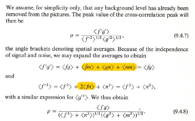
Indicative of the fundamental problems with the Bershad and Rockmore CCC-to-SNR
relation is that their final formula is fatally flawed (SNR=CCC/(1-CCC); Fig 1B). Whereas
the SNR is – per definition – positive, the CCC can assume values from: -1 ≤ CCC ≤ +1. In
the absence of a signal, for example, the CCC oscillates around zero. Any negative value for
the CCC in this formula, directly translates to a negative value for the resulting SNR value,
incompatible with its very definition. This CCC-to-SNR relation therefore could, at best,
only give reasonable SNR approximations in the case where the CCC is very close to
positive unity, that is, for data with a very high SNR value. In information harvesting,
however, we are primarily interested in the case where a small signal emerges from a noisy
background. It is in that limit that the CCC-to-SNR relation fails completely.

 A) B)

 C) D)

 Figure 1: Excerpts from the original CCC-to-SNR papers.
 We reproduced these exact excerpts to show the literal form in which a priori assumptions
 are made in these papers: (A-B) [Bershad & Rockmore 1974]; and in the follow-up papers:
 (C) [Frank & Al-Ali 1975] and (D) [Saxton 1978]. In the latter paper the explicitly deleted
 cross-terms are marked in yellow.

This CCC-to-SNR formula was then copied literally to microscopy in [Frank & Al-Ali,
1975], thus violating the (impossibly) strict boundary conditions of [Bershad & Rockmore
1974]. No justifications were given for this extended applicability other than: “In image

 4

processing application where N is of the order of 10,000, the Gaussian assumption can
therefore be dropped” (Fig 1C). Saxton [Saxton 1978] then provided a comprehensive
derivation of the CCC-to-SNR formula, pinpointing precisely the cross-terms that were
assumed to be zero (“because of the independence of signal and noise”) and which were
taken out of the equations (Fig 1D). In all three papers, the same fundamental mistake was
made: concluding from a zero-expectation value of a cross-term, that each individual cross-
correlation would be zero. Instead of this being an independence assumption, it therewith
became an orthogonality assumption, violating the Central Limit Theorem (CLT), with
serious long-term consequences.

III) Important differences in Fourier-space between 1D and 2D/3D data

As discussed above, CCCs depend on , the number of elements in the vectors to be
correlated. For 1D data, as used in [Bershad & Rockmore 1974], a random white noise vector
translates to a random white noise vector in Fourier-space. In the case of 2D data or 3D data
[Van Heel & Schatz 2005] the noise is also white in a (Cartesian) 2D or 3D Fourier-space.
However, we are interested in data as function of an isotropic spatial frequency, irrespective
of the orientation of the sample within the (Cartesian) 2D image or 3D volume. We are thus
looking at the data in terms of their distance to the origin: in rings in 2D Fourier-space
(Fig 2), or in shells in 3D Fourier-space. In these cases, the number of pixels/voxels in
the Fourier-space rings/shells varies as function of or respectively (Fig 2). Note that
the presence of symmetries in the data reduces the number of independent sampling points
 R in a ring/shell.

The Shannon-Nyquist sampling theorem requires that the sampling frequency for one-
dimensional (1D) data is higher than twice the maximum bandwidth B. For two-dimensional
(2D) and three-dimensional (3D) data, in a Cartesian co-ordinate system, however, the
corresponding maximum bandwidths in the x-, the y-, and z-directions (Bx, By, Bz), are not
the bandwidths we are interested in primarily. The maximum isotropic bandwidth, in the 2D
case, has a ring shape (up to touching the edges of the square 2D Cartesian Fourier-space).
The Shannon-Nyquist sampling rule – in a strict isotropic interpretation – therefore demands
that the rest of this Cartesian Fourier-space remains empty (the area beyond the disk-shaped
Br bandwidth). No information may be present in the corners of this Fourier-space since that
would make the orientation of an object in the Real-space image anisotropically influence
its representation. Thus, in the Cartesian Fourier transform of 2D images, at least ~22% of
the outer area must remain empty in order to comply with this isotropic 2D sampling rule.
In the 3D case, the maximum isotropic bandwidth has the shape of a sphere inscribing the
cubic 3D Cartesian Fourier-space. Here also, we require that the Fourier-space stays empty
beyond the Br bandwidth sphere: at least ~48% of that sampling cube (the corners) must
remain empty. We have not yet seen this issue discussed in the literature.

 5

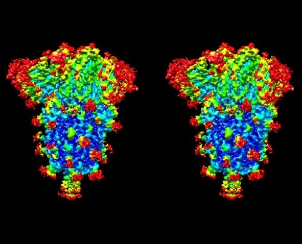
Figure 2: In a Cartesian 2D (or 3D) Fourier-space, the sampling is in the X, Y, (and
 Z,) directions. This Cartesian sampling scheme is not uniform as function of spatial
 frequency r. Therefore, the sampling rings far from the origin (high-frequency data
 components) have many more sampling points N1 than the low-frequency N2 sampling
 rings closer to the origin. This issue is of crucial importance in understanding the noise
 and signal contributions in spatial-frequency dependent metrics. Close to the origin,
 the number of sample points Nr in a ring/shell drops to just a few. As a consequence,
 the inner products of signal or noise vectors have a large relative variance, which is
 very relevant for determining FSC-resolution thresholds (see main text).

IV) The sampling theorem is valid in Real-space AND in Fourier-space

The Shannon-Nyquist sampling theorem in Real-space requires that the power spectrum of
the measurement being sampled drops to zero prior to reaching the (isotropic) Nyquist
frequency. In Real-space this means that we cannot have abrupt changes in the measured
densities such as a sharp mask delineating an object of interest, or just the sharp border of
the Cartesian sampling space cutting away the measured densities. Any such sharp changes
in Real-space will lead to the power spectrum in Fourier-space exceeding the Nyquist limits
and introducing wrap-around artefacts. We used this classical Shannon-Nyquist sampling
theorem explicitly in criticising the CCC-to-SNR formula boundary conditions in [Bershad
& Rockmore 1974]. To comply with the sampling theorem, neighbouring sampling points
in Real-space must necessarily be correlated.

It is, however, not enough that the power in Fourier-space gradually drops to zero prior to
reaching the (isotropic) Nyquist frequency! In fact, the measurements in neighbouring
sampling points in Fourier-space must also be correlated for the same reason that
neighbouring sampling point in Real-space must be correlated. In Fourier-space the
measurement will normally be sampled with the same number of sampling points as the

 6

measurements in Real-space (keyword: Fast Fourier Transform: FFT). From the Fourier-
space measurement’s perspective, the Real-space measurement is just its Fourier transform!
By the very same Shannon-Nyquist sampling rule, we thus cannot allow for Real-space
intensity components to exceed the original (Cartesian) sampling-space boundaries. Such
overstepping of the boundaries in Real-space will also cause aliasing (wrap-around)
artefacts, but now in Real-space. In terms of the Real-space measurement, the object or
“area-of-interest” must thus also be contained within the central part of the sampling space
and the information must be apodized to zero prior to reaching the edges of sampling space.

This sampling rule is the Fourier-space equivalent of the classical Shannon-Nyquist
sampling rule requiring that all Fourier-space power must have gradually dropped to zero
prior to reaching the (isotropic) Nyquist frequency. A rule of thumb in signal processing is
to limit the data in 2D/3D Fourier-space to, say, ~2/3 of the Nyquist frequency. The Real-
space equivalent of that requirement is that the object of interest should be contained within
~2/3 of the Real-space inner radius. The sampling theorem is thus a Janus-faced theorem
with one face in Real-space and one face in Fourier-space! In both spaces there cannot be
any power left anywhere close to the (isotropic) edges of the (Cartesian) sampling space in
order to properly represent the data. We call this the Janus apodization rule. This rule has
direct links to the Gabor-Heisenberg uncertainty principle [Gabor 1946; Hsieh 2016]. In
both Real-space and Fourier-space, the sampling must be fine enough to be able to
sufficiently sample the smallest relevant detail, which, in turn, is related to the overall spread
of the data in the conjugate space by the Gabor-Heisenberg uncertainty principle.

To illustrate the consequences: A Real-space spherical object like an 666Å-diameter
icosahedral virus, sampled at 1.0Å3 / voxel, must best be contained within a box with edges
of at least 1000Å. Thus, in Real-space, only (4/3·π·3333Å3) of the 109Å3 voxels, may be
occupied. That implies only ~15% of the Real-space voxels may contain information for the
data to not violate the ad hoc ~2/3rd Nyquist sampling rule, and that requirement is matched
by the equivalent requirement applying to the power distribution in 3D Fourier-space.

V) Traditional thinking about signals, noise, SNRs, and CCCs

We now focus on the classical measurement consisting of a fixed signal deteriorated by
an independent additive noise ; their respective powers being: and . The traditional
“saloppe” way of thinking about this is that, because of the independence of signal and noise,
the overall variance or the power of measurement = + , is given by its square: ≈
 + , assuming that the signal and the noise are independent. The SNR definition then
follows equally saloppe as: = / . However, this over-simplification leads us in a
conceptually incorrect direction, when looking at the cross terms between signal and noise,
and when discussing the concept of information.

The SNR of a measurement always depends on the integration time used for attaining that
measurement of an incoming noisy signal. Let us for simplicity first assume that we submit
the incoming intensities to an integration time to obtain measurement ( ). If we integrate

 7

the random-noise deteriorated signal over time , the random-noise components average to
a relatively lower value, while the signal, during that time , averages to a relatively higher
value. The associated = / value thus increases as function of an increased
integration time . There is no such thing as an SNR value of a source without considering
the integration time applied for collecting the vector ( ). Again, the SNR is a property of
a specific measurement ( ), collected with integration time , and not an intrinsic property
of the incoming noisy signal. (The same applies to the CCC, as stated in the introduction.)

In the single particle cryo-EM example, this integration time τ contains two elements:
a) the integration time in terms of electron counts per pixel used to collect an image, and
b) the number of identical particle images averaged to form the measurement vector.
In the latter case, if one were to average an infinite number of particle images, the noise
would average out and the SNR of the measurement would be infinite, through the division
by the 0 noise. The SNR issue will be elaborated upon in chapter VIII, below.

The variances and co-variances of an additive-noise-deteriorated signal are defined through
the correlation values between two measurement vectors and , as in:

 = ( ) · ( )
 = { ( ) + ( )} · { ( ) + ( )} ( ).
 = ( ) + ( ) · ( ) + ( ) · ( ) + ( ) · ( )

There are four (cross-) terms to be considered. The first and most straight-forward term is
the square of the constant signal ( ); for a signal vector of length the power thus becomes
proportional to . The second term is the inner product between two independent noise
vectors ( ) and ( ). The inner product of two random vectors of (sufficient) length 
is given by the Central Limit Theorem (CLT) [Wikipedia] and yields: . This is because
the two random vectors and have the same standard deviation n. For the same CLT
reason, the cross terms between signal and noise ( ) · ( ) and ( ) · ( ) together yield
an expected power of · · .

The fact that the two independent random noise vectors and yield a power contribution
proportional to has never been disputed. However, the inner products between a signal
vector ( ) and an independent noise ( ) have, strangely enough, mostly been taken out
of the equations, using the same argumentation as used for the noise-to-noise correlations,
namely, that those two vectors are independent or uncorrelated. These authors therewith
defined any noise vector and the signal vector to be orthogonal (zero inner product).

VI) Inventory of methodological issues discussed so far

(A) The Shannon-Nyquist sampling theorem (in 1D) requires that a signal is sampled at a
 frequency higher than twice the bandwidth . This implies that the power of the signal
 must gradually drop to zero prior to reaching the Nyquist frequency in Fourier-space.

 8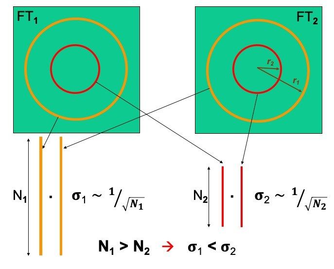

(B) Sufficiently sampled band-limited data will, because of (A), exhibit correlations
 between neighbouring sampling points in Real-space.

(C) Two random-noise vectors will have an inner product with a standard deviation
 proportional to √ ; where is the length of those vectors. This is because the two
 vectors are statistically independent (keyword: Central Limits Theorem, CLT).

(D) The inner product of a noise vector and a signal vector will also have a standard
 deviation proportional to √ because of their independence (using the same CLT
 argument (C)). Seen from the noise vector, the signal is just another noise vector.

(E) For 2D/3D data, the radius dependency of in Fourier-space must enter into the
 equations explicitly since that does not come naturally in a Cartesian sampling space.

(F) Any symmetry creates repetitions in the data. The number of effective voxels Nr must
 be balanced against the number of symmetrical repeats.

(G) Isotropicity, together with the Shannon-Nyquist sampling rules, requires that for 2D
 and 3D data the Fourier-space power approaches zero prior to reaching the maximum
 inner radius . For an isotropic data representation, the excess space must remain
 empty beyond that radius up into the corners of the Cartesian sampling space.

(H) The Janus apodization rule, a direct consequence of the sampling theorem, requires
 that measurements in Real-space are apodized to zero towards the edges of the
 sampling space, just as their power in Fourier-space must drop to zero in time (A).

VII) The accumulation of flaws over time

Resuming: The CCC-to-SNR idea introduced by Bershad and Rockmore [Bershad &
Rockmore 1974] included contradictory boundary conditions in Fourier-space (A) and Real-
space (B, H) making the theory not applicable in practice. The orthogonality assumptions
imply that all cross-terms (C) and (D) were zero. Such mathematical a priori assumptions,
requiring abrupt changes in the data both Real-space and in Fourier-space, are unphysical
while violation the Gabor-Heisenberg uncertainty principle (and the CLT). Frank and Al-
Ali [Frank & Al-Ali 1975] copied the CCC-to-SNR formula literally to the field of
experimental image processing, ignoring those boundary conditions arguing that Real-space
images are large (N>>1), thus implicitly accepting (A-D, and H). Moreover, Frank and Al-
Ali applied the formula in 2D Fourier-space (E), where the number Nr can be very small
when close to the origin (Fig 2). Saxton [Saxton 1978] assumed explicitly that the
independence of signal and noise (D) justified removing the cross-terms. Removing those
terms, however, assumes those vectors are orthogonal, not independent. The argumentation
(E) in [Saxton and Baumeister 1982] that Nr is a function of R in 2D Fourier-space is correct.
The influence of point-group symmetry (F) entered the discussion in [Orlova 1997] and was
supported by unambiguous computational model experiments in [Van Heel & Schatz 2005],

 9

an argument mostly ignored by cryo-EM workers. An ad-hoc 0.5 FSC threshold, introduced
in [Böttcher 1997], was endorsed in [Malhotra 1998]. However, that justification ignored all
arguments (A-F) and did not provide credible arguments for that specific fixed threshold
value. The new issues (G-H) had not yet emerged, and were obviously also violated.

The main problem in this chronological list remains the intrinsic orthogonality assumption
(D) which was also used to deny the radial-dependency argumentation (E). These basic
issues have been negated/ignored in many more recent methodology discussions and
especially in [Rosenthal & Henderson 2003] in which paper the popular, yet incorrect, 0.143
threshold for the FSC was postulated. In that paper all arguments (A-F) were declared
inappropriate using incomprehensible circular logics – no citations provided – such as:
“However, a map with or without symmetry will be equally interpretable when the FSC is the
same. Any threshold criterion that depends on the number of pixels in the map is not an absolute
criterion for the evaluation of resolution”.

In our supplementary materials we perform a simple model calculation in which we refute
this orthogonality assumption (D). Our minimalistic counter example contains exactly the
elements postulated in all theoretical papers, namely, that the two 3D volumes to be
compared, contain the same signal but different realisations of additive random noise. The
advantage of such model calculations, is that we know a priori what part of the correlations
represent signal and what part noise. It is thus simple to assess the influence of each cross-
term separately! Our model calculations show that the largest noise contributions stem from
the cross-terms between the signal and the random noise, thus refuting most papers on the
issue. Typically, the cross-terms are dismissed in their first mentioning, like in: “Assuming
signal and noise are uncorrelated, and for data on the same scale, the above expression may
be written as follows: …” (cited literally from: [Rosenthal & Henderson 2003]).

The fact that those cross-term contributions actually represent the largest noise contributions
makes perfect sense. Since we are especially interested in the information carried by signals
that are larger than the background noise, these s·n cross-terms will represent a larger noise
contribution than will the pure noise-to-noise cross terms, at the critical frequencies. A
sobering aspect of such methodological errors surviving for so long in the literature is that
second- and third-generation methods appear in which errors have accumulated with time.
An example is the recent trend towards claiming reproducible resolution levels very close
to the Nyquist frequency. Such under-sampling of the data adds a violation of the sampling
theorem (G), while using the FSC metric beyond its validity range, and using a refuted 0.143
threshold, which itself violates all arguments (A-F) listed above, etc.

VIII) Your Signal-to-Noise Ratio (SNR) may not be what you think it is

Having shown that the formula used for estimating SNR values from CCC measurements is
wrong, the question arises whether the formula can be corrected! Unfortunately, that is
impossible because of the fundamentally different nature of the CCC and SNR metrics. The
CCC can always be measured, the SNR, in contrast, is a positive-definite target that is not

 10

measurable, failing the exact a priori knowledge of the original signal. The historical
motivation for deriving the SNR from the CCC stems from the general belief that SNRs are
universal information metrics, a reputation we will here put under scrutiny.

The SNR, as a quality metric, can only make some very limited sense within one experiment
with otherwise constant experimental conditions. It cannot serve for comparing the results
of independently conducted experiments. As a simple counter example: if one bins a normal
noisy image of 4096x4096 pixels by averaging 2x2 pixels into one, the SNR of the resulting
2048x2048 pixel image will typically increase significantly! Normal images contain strong
low-frequency signal components, and significant high-frequency noise components. Thus,
by reducing the number of pixels through binning, the SNR of the image will increase even
though this will necessarily also cut out any high-resolution signal information present in
the data. This simple example illustrates that the SNR is not a useful metric for characterising
the information content of an image. In other words, the often-seen generic statements like:
“Our algorithm X works well for images with a SNR level above M”, have no absolute
meaning. They cannot be used to support claims that algorithm X is better than algorithm Y
because it still works at lower SNR levels [Wikipedia SNR].

The SNR can also be defined in Fourier-space in the form of a Spectral SNR (SSNR) [Unser
1987]. In Fourier-space the arguments for a frequency-dependent SSNR are significantly
more favourable than for a Real-space SNR. When a Real-space image is binned from
4096x4096 pixels to 2048x2048 pixels, for example, the central part of the 2D Fourier
transform of image remains virtually unchanged for both the signal and the noise part of the
data and therefore the SSNR at low frequency also remains unchanged. The low-frequency
rings used for FSC calculations (Fig 2) also remain constant, a reason why the FSCs are
also stable for sufficiently sampled data. However, even when we focus on the SSNR, we
cannot compare the results of different experiments on the same scale. For example, when
using the same-sized images in Real-space, but gradually reducing our area of interest by
masking, the SSNR in Fourier-space will increase gradually! This is because of the
increasing correlation levels in Fourier-space. In its extreme limit, the area of interest will
be a single point in the centre of the Real-space image and its Fourier transform will
therefore be a constant everywhere in Fourier-space. The SSNR will then become infinite
for all frequencies f, whereas any information metric should then asymptotically yield zero.
Bottom line: SSNRs are not information metrics, not in Fourier-space and not in Real-space!

IX) Information is maybe also not what you think it is

The Signal-to-Noise ratio (SNR) concept originated primarily in electrical engineering and
was designed to quantify how well a channel (a telegraph line, or a telephone line) transports
a known input signal to its output, in spite of noise sources deteriorating that signal
underway. In other words, the popular SNR is associated with the loss of the information
when a known signal is transmitted through a channel. The fact that the SNR is a positive
function already indicates that one assumes a-priori that there is a signal at the input of the
channel. In data-harvesting, the story is different: we are receiving very noisy measurements

 11

at the end of the channel and we wonder whether there is some systematic signal hidden in
that noise. We are interested in collecting information we knew nothing about to start with.
We thus rather need metrics that measure how much information has been harvested from a
source, not how much information has been lost since a known message left the source.

Real-space SNRs may be useful ad-hoc metrics in electrical engineering to describe the
transport of known information from A to B, but they cannot be used to quantify small
signals emerging from a background of noise. Even in the absence of a signal, the outcome
of any SNR measurement must – per definition – be positive! Information theory was
developed from that same perspective: how much of the known signal is lost by transporting
it through a noisy channel. As per Shannon’s famous rule of thumb [Shannon 1948], the
information capacity of a channel is assumed to be: ≈ ⋅ ( + / ).

Shannon himself defines the white additive noise to be independent of the known signal in
terms of noise power being independent of the signal power . We note that defining
the noise power to be independent of the signal power is a very different from defining the
noise n to be independent of the signal s. This is because the noise-associated power
components in a recorded intensity, will contain three cross-terms, as discussed above
(chapter V). Of these cross-terms, the most important cross-terms are those between signal
and noise: · and · (see appendix). Shannon’s choice defines the signal versus noise
cross-terms to be non-existent from the start. That definition must be seen in the context of
the deterministic physics of around the turn of the 19th to the 20th century when the attitude
was one of, we know it all and don’t want to lose what we know. It is however, not
compatible with more modern physics encompassing wave-particle duality from of
beginning of the 20th century, where the square of the wave function determines the
probability of finding an arriving photon or electron.

We are now facing a serious problem: the metric everybody associates with information
and information collection, the SNR, is a definite positive metric that can actually not be
used to measure new incoming information. Since this metric is defined as a positive entity,
that makes it impossible for it to not collect information, even if there is none to be recorded.
The CCC, in contrast, can always be recorded and it will naturally oscillate around the zero
value in the absence of a signal. When deriving the SNR, through the experimental CCC-
to-SNR formula of [Frank & Al-Ali 1975], the SNR is then also forced to oscillate around
the zero mark, in violation with the very definition of the SNR. The SNR can thus– at best
– be used to assess the loss of information. As a consequence, Shannon’s information
measure also can also only – at best – be used to define the loss of information, as per the
Shannon-Hartley theorem on the channel capacity [Wikipedia Shannon]. How to resolve
this conundrum? The solution is to start all over again, and create a new information metric
based on the measurable and well-behaved CCC rather than on the evasive SNR. We can
thus create a metric that covers both aspects of signal processing: measure the information
lost in a noisy channel, or measure new information harvested from a noisy source.

 12

X) What if you don’t a priori know the signal we are looking for?

Let us assume we want to collect a signal/message we know virtually nothing about prior to
the experiment. Say, we purified a small protein and prepared it on an EM grid which we
then imaged in an electron microscope. We have no idea whether the small protein will
actually stick to the grid and what it will look like. We are thus essentially entering the
territory of SETI logics (Search for Extra Terrestrial Intelligence). To grab our attention, the
extra-terrestrials could choose to modulate some strong radiation source with a signal, which
they would then probably repeat to emphasize that the message is intentional. We humans
would then be trying to make sense out of the noisy measurements by searching for multiple
copies of the message using correlation techniques [Harp 2018]. Periodic repeats of a signal
will especially catch our attention (see for example [Amiri 2020]). Recognising a protein in
a cryo-EM sample is probably simpler than trying to understand extra-terrestrial messages:
in the case of a small protein we already have a good a priori idea of what a small protein
would looks like in the microscope. However, trusting too much on what you think the
answer will be is by itself risk-prone, as we will discuss below.

An important first parameter for data collection is the integration time τ within the
transducer: each pixel of a camera – a 2D image transducer – is an independent 1D signal
transducer. This recording phase is then followed by a detection-phase and an alignment-
phase (also known as phasing) of the received measurements. At this time, we still don’t
know whether we have recorded some useful information in the noisy data. One can detect
the presence of messages/objects in the incoming noisy measurements by detecting peaks in
the local modulation or the local variance of the incoming noisy measurements [Van Heel
1982, Burgess 1999], or using correlation functions like: cross-correlations [Saxton 1976,
Van Heel 1992]; auto correlations [Harp 2018]; or triple-correlations [Kam & Gafni 1985].

Having collected what we think is useful information, we then reach a fundamental aspect
of collecting unknown information: the apparently relevant new information needs to be
validated. Control experiments running parallel to the results experiment are of fundamental
importance to verify that genuine information has indeed been collected. When authors work
towards a preconceived result, science becomes very tricky. We call attention to the
exchange in PNAS on cryo-EM structures of the HIV outer-membrane trimer, a primary
drug target for the prevention of HIV infections. Mao, Sodrosky, and co-workers [Mao
2013] had published papers on that structure that were questionable given their processing
approach. Their papers were refuted in three PNAS papers [Subramaniam 2013, Henderson
2013, Van Heel 2013]. Mao and co-workers appeared to have been working towards a
preconceived answer (“Looking for Einstein in random white noise. The criticised work has
since been superseded by a number of reliable high-resolution structures by others, but the
contested papers have still not been withdrawn. This controversy illustrates that it remains
difficult to prove a falsehood, especially when the underlying data is not available. When
looking for something specific in random noise, one will always find matches. These
techniques must be used conscientiously and be properly validated. Objective metrics help
defining what information has been collected and help prevent misuse. As an introduction
to our new metrics, we first discuss the classical Fourier-space correlation metrics.

 13

XI) The FRC and FSC metrics

The CCC has always been a very popular metric in signal and image-processing, in spite of
its disadvantage of being indiscriminative in the case of 2D and 3D data processing. Fourier-
space versions of the CCC like the FRC/FSC were proposed for that reason: they are much
more detailed than the Real-space CCC, since they are calculated for each resolution interval
separately (Fig 2). The principle behind those Fourier-space metrics is the same as for the
CCC: to compare two signals by cross correlation. The FRC/FSC metrics have become very
popular in structural biology, but they are general metrics that can be applied everywhere
2D or 3D data is being collected or compared. They are now proliferating to all fields of 2D
image science and 3D tomography. The FRC was first used to compare the results of
negative-stain EM with the results of X-ray crystallography of the same molecule [van Heel
1982]. The FSC was first used for comparing different 3D-reconstruction algorithms
[Harauz 1986]. The FRC/FSC is a cross-correlation coefficient, in which the cross
correlation is normalised by the square-root of the power in the corresponding rings/shells
in Fourier-space (Fig 2). The FSC is defined as:

 ∑ ∈ ( ) ⋅ ∗ ( )
 ( ) = ( ).
 √∑ ∈ | ( )| ⋅ ∑ ∈ | ( )| 

Although the product { 1 ( ) ⋅ 2 ∗ ( )} yields a complex value, its integral over each
shell/ring gives a real result, of the Hermitian symmetry of the data. The FSC is thus a real-
valued metric, fully equivalent to the Pearson cross-correlation coefficient. When the two
volumes to be compared are identical, the FSC yields a value of +1, over all spatial
frequencies. When, in contrast, one volume is the negative version of the other, the FSC
comparison yields a -1 over all spatial frequencies. The general behaviour of this metric has
been described elsewhere in extenso (cf. [Van Heel & Schatz 2005]).

The FRC/FSC has historically been used mainly as a metric for resolution assessment. But
for what kind of resolution? We distinguish two main types of resolution. Firstly, there is
the instrumental resolution of an imaging device like a light microscope, which would be
determined by the physical properties of the instrument such as the numerical aperture of
the lens and the wavelength of the light (electrons) used [Goodman 2004]. The instrumental
resolution will ideally have a constant value over the whole object plane (isotropic imaging).
The instrumental resolution is a characteristic of the instrument, that is valid even when the
device is switched off and safely stored in a cupboard. In the 1D case one would speak of,
say, the bandwidth of an audio amplifier, but the whole idea is the same: defining the
properties of the linear system, independent of the specific signals it transfers.

The FRC/FSC type of resolution metrics, in contrast, are primarily intended to assess the
resolution actually achieved for a given sample: we call those the results resolution. They
focus on the object we image and can refer to one specific data-collection experiment. If one
here forgets to switch on the illumination, the results resolution will be very bad indeed.

 14

Since the objects of our attention will typically be smaller than the size of the object plane,
the results-resolution will not be isotropic over the instrument’s field of view. The object
plane beyond the object of interest, may even be masked off. All FRC/FSC results
resolutions are thus de facto local resolutions when compared to an isotropic instrumental
resolution. We tend to nevertheless call the FRC/FSC results-resolution of an area
containing the full object of interest, a global resolution. The FRC/FSC results resolution
may be limited by the instrument’s maximum resolution, but in most cases the results
resolution is more likely to be limited by, say, the radiation sensitivity of a decaying sample.
Moreover, the results resolution can be compromised locally within the object, such as a
full-chest tomogram, which may be blurred locally by the movement of a beating heart.

When we gradually mask off an area in Real-space to focus on a smaller area within the
object of interest, the number of independent voxels in Fourier-space will be reduced due to
the increasing influence of the convolution with the Fourier transform of the decreasing
Real-space mask. The smaller number of independent voxels in each shell, Nr, must be
properly be taken into account as was done for the ½-bit threshold criterion [Van Heel &
Schatz 2005; 2017]. Similarly, when dealing with a structure with a high degree of
symmetry, that symmetry is also reflected in information duplications in Fourier-space. The
influence of these effects enters through the ½-bit threshold function, which is a function of
the effective number of voxels NR at each radius (Fig 2-3).

 A) B) C)

 Figure 3: The FSC used globally and locally.
 The FSC, in combination with the ½-bit threshold function [Van Heel & Schatz 2005],
 make global and local resolution values comparable on the same scale. All three curves
 show a ½-bit cut-off at ~1/0.27=3.7Å, although the threshold levels differ for the
 global FSC (A) and the local FSCs (B-C) (from [Van Heel & Schatz 2017]).
 A) FSC calculated for two full 3D volumes (3603 voxels, 0.6 Gaussian mask)
 B) FSC for two corresponding 3D sub-volumes (243 voxels, 0.6 Gaussian mask) cut
 out from the volumes used in A).
 C) FSC calculated for two other corresponding 3D sub-volumes (again: 243 voxels,
 0.6 Gaussian mask) cut from the volumes used in A).

 15

XII) The new FRI and FSI metrics

When the FSC/FRC curves get very close to their -1 or their +1 limits, they no longer reflect
the similarity level between the two measurements proportionally. A 1% difference in value
between an FSC(ri) of 0.99, and one of 0.999, does not correctly reflect their huge
significance difference. To compensate for this disproportionality, we apply a Fisher
transform [Fisher 1915, Wikipedia Fisher], to the FSC or FRC. The resulting function we
call the Fourier-Shell-Information FSI, or Fourier-Ring-Information FRI respectively:

 + ( )
 ( ) = · { } ( ),
 − ( )

(see: Figs 4,5). The constant K in this equation is a proportionality/calibration constant with
a real physical meaning, equivalent to the bandwidth B in the Shannon-Hartley channel
information capacity ( = ⋅ { + / }). The constant K will be discussed in
more detail below. An alternative form of equation (3), emphasising the similarity to Real-
space Shannon-Hartley channel information capacity is:

 · ( )
 ( ) = · { + } ( ).
 − ( )

The FSI(ri) information metric is closely related to the FSC(ri) at the same radius, but is
now measured directly in bits, thereby eliminating the need to define a separate threshold
curve. Note that these FRI and FSI information metrics are, like the FSC and FRC, subject
to the rules and boundary conditions listed above, including the Janus apodization rule,
requiring the power in the data to drop off to zero towards the (isotropic) edges of the
sampling space, not only in Fourier-space but also in Real-space. Let us now scrutinize the
behaviour of the FSI. First, in the limit of the FSC approaching the zero mark, the FSI also
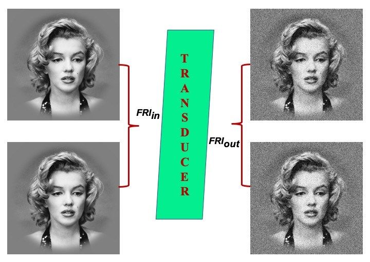
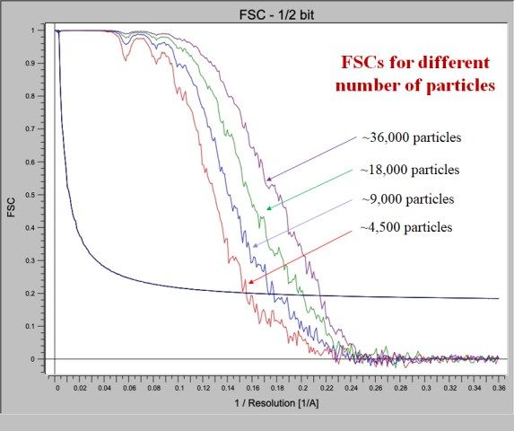
goes to zero (because for |x|

Figure 4: Information harvesting in a Linear System.
 In linear systems, given a deterministically known object (here a portrait of Marylin
 Monroe by Richard Avedon), the output image can be predicted, provided we know
 the transfer properties of the linear system. Associated with this Gedankenexperiment
 is – in the absence of noise – the concept of the instrumental resolution. It is, of course,
 unphysical to ever have a deterministic knowledge of an object because all information
 we have on the object stems from the noisy output images we have collected previously
 through the noisy linear imaging system. We can accumulate all images collected in an
 experiment into two half-dataset sums to then compare them in Fourier-space by
 Fourier Ring Correlation: FRC (Fig 2). The FRC increases with an increasing number
 of images being summed but it soon reaches a maximum plateau at the level 1. More
 useful is to express the harvested information operating on a logarithmic scale, using
 the proposed Fourier Ring Information FRI metric.

To illustrate the procedures, we use an arbitrary, large experimental dataset resulting from
standard cryo-EM procedures such as explained in [Afanasyev 2017]. The importance of
having a large experimental dataset is that we can split it into smaller sub-sets. As long as a
dataset is in a noise-limited regime, a doubling of the size of that dataset leads to a doubling
of the amount of information collected at that resolution level! At resolution levels where
we already have collected much information the increase in information harvested becomes
logarithmic and the doubling of the data set thus leads to a linear information increase. From
a large dataset with ~36000 aligned molecular images, we randomly extracted four different
sub-groups, containing: 4500, 9000, 18000, and 36000 images, respectively. The FSC and
FSI results from each of these four experimental datasets are shown in the same graphs, to
the same scale (Fig 5). Different methods/algorithms discussed in this paper were used to
generate the different plots (Fig 5B-C-D).

 17

A B

 C D

 Figure 5: Behaviour of the FSC, the FSI and the FSIr, as function of dataset size.
 A) The FSC curve starts off close to the maximum value of 1 and gradually drops to a low
 value oscillating around the zero mark. Oscillations close to the origin are due to the small
 number of voxels in that area (Fig 2). A threshold curve indicates where enough data was
 collected for a reliable interpretation (the ½-bit resolution threshold).
 B) The FSC curves for four different groups of the dataset (1/8th; 1/4th; 1/2; and full dataset),
 calculated, with explanatory markings. The orange line, shows maxima of the FSCs very close
 together, close to the “1” maximum. The four coloured vertical lines assist in the mutual
 comparison of the FSC, the FSI and FSIr metrics resolution thresholds.
 C) The FSI curve starts at the zero and increases gradually. The FSI at low resolution, however,
 still gives a too strong representation of the poorly defined low-frequency data (red circle).
 D) The r2-weighted FSI (FSIr) gives the best representation of the collected information as
 function of spatial frequency. The brunt of the collected information is here seen in the mid-
 spatial frequencies, a frequency range where the amount of information collected increases
 rapidly with an increasing size of the dataset (see main text).

The four FSC curves in (Fig 5A-B) are all visually touching the 1 maximum, at around the
1/5th of the Nyquist frequency, marked with a vertical orange bar (Fig 5B). The four FSI

 18

curves (Fig 5C) are already showing a 30% vertical variation at 1/5th Nyquist. Moreover,
for the FSC, the resolution threshold idea applies only in combination with the ½-bit
threshold curve. In the case of the four FSI curves, however, the curves themselves reflect
the information level achieved at each frequency. Any horizontal line will have an
information content interpretation (Fig 5C). Note that the straight-line threshold (Fig 5C)
on the four FSI curves closely match the ½-bit threshold curve crossing points on the
corresponding FSC plots. On the low-resolution end, close to the origin, the FSC already
oscillates away from the expected maximum value of 1 due to the small number of sampling
points (Fig 5A-B). The few very low-frequency components hold very little information.
Those contributions are better reflected in the FSI curves which show a real drop in the
information at the low-resolution information level. The bare FSI, however, directly derived
from the FSC, does not sufficiently reflect the low information content close to the origin.

XIII) Radially weighting the FRI and FSI metrics

The FRC/FSC curves are normalised per ring/shell in Fourier-space to a value between
minus and plus unity. However, the number of sampling points per ring/shell in these metrics
will vary proportional to or . The farther away from the origin, the more information
each ring/shell can contain (Fig 2) and that information capacity needs to be weighted
correctly in information metrics like the FRI/FSI. Other factors like the point-group
symmetry and the limited spatial extent of the objects, are also needed to define the ½-bit
threshold curve [Van Heel & Schatz 2005]. In the 2D and 3D cases, we thus need to weight
the information contributions of the FRI/FSI as function of radius: the FRI must be
weighted by the number of sampling points at each ring , and the FSI must be weighed
by number of sampling points contained in each Fourier-space shell (proportional to ).
These versions of the metrics we call the and the , respectively. An example of
the -weighted , metric is given in (Fig 5D). Note that the and the are the
metrics intended for real use: the unweighted the and the have been introduced
more for didactical reasons. We will thus drop the r subscript in these and will refer to the
radially weighted versions of these 2D and 3D information metrics. However, we must note
here that where the classical ½-bit threshold in the and the become a straight line
through the origin, or a parabolic function, respectively. What becomes more of a horizontal
line with these metrics, are the total amount of information collected per frequency range.

XIV) The constant K contains the radial weight and the κ-factor

The constant K is a proportionality constant with an important physical meaning comparable
to the bandwidth B in the Shannon information capacity, albeit that K is rather associated
with the width of the object, than with the Fourier-space bandwidth B. The constant K has a
broader meaning than the analogue bandwidth B. The closest relative of K is the historical
number of degrees of freedom introduced in [Gabor 1961] and in [Toraldo di Francia 1969].
We discussed the influence of the Fourier-space radius ri on the FRI and FSI, where, the

 19

farther from the origin, the more information a given spatial-frequency shell can carry. For
3D data (FSI) we can readily factorise as:

 ~ · ( ),
or, in the case of 2D data (FRI):
 ~ · ( ).

This - or -weighting has become our standard mode of operation and we will mostly
drop the r subscript when no explicit reference is required. Parameter has the interpretation
of a Real-space filling degree. For a three-dimensional object, with a linear dimension D,
within a volume of linear size L, the filling degree is D/L and the value of becomes:

 ( ).
 ~ ( )
 
Similarly, in the 2D-case (images) this formula applies, but using a power of 2. With this
formulation one may first think of a cubic box of width D, within a three-dimensional space
of width L, but sharp edges are not permissible neither in Real-space nor in Fourier-space
since that would violate the Janus apodization rule. We must rather think of a soft-edged
area of linear dimension D containing the object of interest in a Carthesian sampling space
with linear dimension L. The parameter also has a normalisation role to play: in the limit
of the object size D → 0, the information content of the object also approaches zero.

The influence of symmetry in terms of the ½-bit resolution threshold is clear [Van Heel &
Schatz 2005]: in the case of a 60-fold symmetrical viral capsid structure, for example, each
viral image contributes 60 individual noisy images of the asymmetric unit to the final result.
In terms of the total amount information collected, as measured by the FSI, however, the
situation is tricky. With multiple copies of the same subunit in the final 3D results, each
copy will carry the same information. One must thus scale the experiment correctly: while
multiplying the collected information by the number of asymmetric units Nsym, we must
simultaneously reduce the effective size of D to represent only one asymmetric unit. Since
these effects cancel each other out, however, they are best just left out of the equations.

XV) Local Resolution, Local Information Density, and Global Information Content

With the FSC plus ½-bit threshold combination, we have a reliable global as well as local
resolution metric (Fig 3). Better for general use still are the metrics for assessing both
types of resolution as was argued above. Often the most useful metrics in the processing and
interpretation of 3D maps, is the Integrated , whereby we integrate the over all
relevant spatial frequencies, say, from 0.2 to 0.6 Nyquist (see information distribution over
spatial frequencies of Fig 5D). This integrated global information content (GIC) metric
yields a single value for the information harvested on the global object and is suitable as a
target optimisation parameter in iterative refinements. The FSC is often used for this purpose

 20

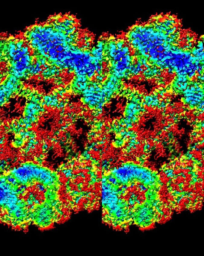
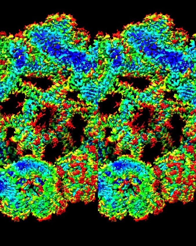
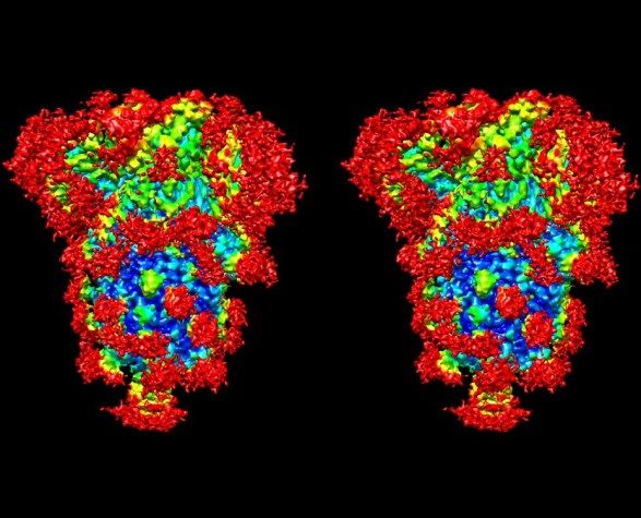
in combination with a specific fixed-value FSC threshold value. However, that is often an
inappropriate combination violating the linearity of processing (see: Discussion).

Used as a local integrated metric, the assesses the local information density (LID) of
a 3D volume as function of position. Because of the integration over the full range of relevant
spatial frequencies, the LID is less sensitive to noise than a local FSC used for local
resolution assessment (Fig 3). The LID can thus be calculated over much smaller local areas
than the local FSC and, although their interpretation is similar, the LID is more “to the
point”! If a 3D volume is (rain-bow) colour-coded by the LID one can directly visualize the
different information levels in different parts of the object and those information levels are
often directly associated with specific physical properties of that type of sample. Those
physical properties could be, for example, the type of tissue in a medical tomogram or the
type of rock-formation in geophysical imaging.

In cryo-EM a high level of information can be associated with rigid structural elements,
whereas low LID values can refer to flexible parts. The LID in the structure of biological
complexes differentiates between different areas of the structures, discriminating between
protein, nucleic acid, phospholipids and glycans, contributing directly to the structural
interpretation of the object. As an example, we used the hemoglobin of Lumbricus terrestris
[Afanasyev 2017]. In the stereo-picture given in Fig 6A-B the LID is directly associated
with the structural properties of the hemoglobin. The dark-blue areas of the map are strong,
high-density beta-barrel structures that form the rigid mechanical backbone of this biological
structure. The red areas are primarily the more flexible parts and especially the
glycosylations on outer parts of the complex. By depicting the map at different threshold
levels, one can directly follow how the glycosylation extends, filling much of the remaining
space between the 1/12th subunits [Afanasyev 2017].

Our new metrics thus allow the assessment of the local information density, given the
availability of two half dataset volumes. We can also apply these metrics for a cross-
comparison between two independent volumes of identical or closely related-structures,
provided the structures are properly aligned and sampled at a sufficiently high sampling rate.
We call the resulting information map local cross information density (LCID).

In an ongoing study, we compare cryo-EM structures of the S-protein of the SARS-CoV-2
virus which have been deposited in the Electron Microscopy Data Bank [EMDB]. These S-
protein trimer structures have mostly been released without supporting validation
information such as half datasets or FSC curves, such that they cannot be verified
independently. (The L. terrestris hemoglobin half-datasets (Fig 6A-B) were also not
available through the EMDB entry emd-3434, but were already in our possession). Most
deposited S-protein trimer densities are under-sampled for the claimed level of resolution,
since they do not adhere to the sampling rules discussed above. Most released structures
have also been refined by iterative non-linear procedures to boost their 0.143-threshold
based FSC resolution assessment but breaking the linearity prerequisite.

 21