The agricultural impact of the 2015-2016 floods in Ireland as mapped through Sentinel 1 satellite imagery
←
→
Page content transcription
If your browser does not render page correctly, please read the page content below
Research Article • DOI: 10.2478/ijafr-2019-0006 IJAFR • 58 • 2019 • 44-65

                Irish Journal of Agricultural and Food Research

                The agricultural impact of the 2015–2016 floods in
                Ireland as mapped through Sentinel 1 satellite imagery
                R. O’Hara1,2†, S. Green1, T. McCarthy2

                1
                    Teagasc, Ashtown Food Research Centre, Ashtown, Dublin, Ireland
                2
                    National Centre for Geocomputation, Maynooth University, Maynooth, Kildare, Ireland
Abstract
                The capability of Sentinel 1 C-band (5 cm wavelength) synthetic aperture radio detection and ranging (RADAR) (abbreviated
                as SAR) for flood mapping is demonstrated, and this approach is used to map the extent of the extensive floods that
                occurred throughout the Republic of Ireland in the winter of 2015–2016. Thirty-three Sentinel 1 images were used to map
                the area and duration of floods over a 6-mo period from November 2015 to April 2016. Flood maps for 11 separate dates
                charted the development and persistence of floods nationally. The maximum flood extent during this period was estimated
                to be ~24,356 ha. The depth of rainfall influenced the magnitude of flood in the preceding 5 d and over more extended
                periods to a lesser degree. Reduced photosynthetic activity on farms affected by flooding was observed in Landsat 8
                vegetation index difference images compared to the previous spring. The accuracy of the flood map was assessed against
                reports of flooding from affected farms, as well as other satellite-derived maps from Copernicus Emergency Management
                Service and Sentinel 2. Monte Carlo simulated elevation data (20 m resolution, 2.5 m root mean square error [RMSE]) were
                used to estimate the flood’s depth and volume. Although the modelled flood height showed a strong correlation with the
                measured river heights, differences of several metres were observed. Future mapping strategies are discussed, which
                include high–temporal-resolution soil moisture data, as part of an integrated multisensor approach to flood response over
                a range of spatial scales.
Keywords
                Agriculture • flooding • Landsat • mitigation • remote sensing • Sentinel

Introduction

In the winter of 2015–2016, the British Isles were struck by                                Efficient monitoring of flood events is fundamental to minimising
a series of devastating storms, which brought extensive and                                 the impact on life and property. Satellite remote sensing, due
persistent flooding to many areas. In the Republic of Ireland,                              to its wide field of view and continuous coverage, is widely
the volume of seasonal precipitation was unprecedented.                                     used in flood mapping and monitoring. The Sentinel 1 mission
Three major winter storms in December 2015 (storms                                          is ESA’s most recent synthetic aperture C-band radio detection
Desmond, Eva and Frank) resulted in >50% of synoptic                                        and ranging (RADAR) (abbreviated as SAR) satellite with flood
stations reporting their wettest winter on record. Stations in                              mapping capability (Malenovský et al., 2012; Amitrano et al.,
the South and Midlands had >350% their long-term average                                    2014), continuing the work of the earlier European Remote
(LTA) precipitation (Met Éireann 2016a, 2016b). Nearly 50%                                  Sensing (ERS) and Environmental Satellite (ENVISAT) missions.
of river gauges operated by the Office of Public Works (OPW)                                Now fully operational, the Sentinel 1 mission deploys two polar-
reported their highest-ever river heights (National Directorate                             orbiting satellites that can map surface water and flood water
for Fire and Emergency Management, 2016). The heavy rains                                   at 10 m spatial resolution every 6 d. Several additional SAR
also brought extensive pluvial floods to the saturated ground                               satellite missions (e.g. ALOS-2, RADARSAT-2 and TerraSAR-X)
beyond traditional floodplains. During Storm Desmond, the                                   also provide flood mapping capability (Arnesen et al., 2013;
European Space Agency (ESA) Copernicus Emergency                                            Bolanos et al., 2016). These and other RADAR missions
Management Service (Copernicus EMS) began monitoring                                        contribute information to Copernicus EMS projects globally. In
flood development at several at-risk towns to provide high-                                 addition to flood delineation, SAR has been used elsewhere in
resolution spatial data to assist in emergency response. Rural                              surface hydrology to estimate surface soil moisture (Moran et al.,
parts of the Midlands and Western region, areas not routinely                               2004), to monitor river stage (Schumann et al., 2009) and to
monitored by Copernicus EMS, were already flooded before                                    map preferential hydrological pathways (Manfreda et al., 2011).
Storm Desmond and would continue to be for several weeks.                                   The use of optical and microwave satellite systems to map

†
    Corresponding author: R. O’Hara
E-mail: r_o_hara@yahoo.com

                                                                                                                                                               44
                                                                          Bereitgestellt von St. Patrick's College, Maynooth University | Heruntergeladen 21.10.19 12:57 UTC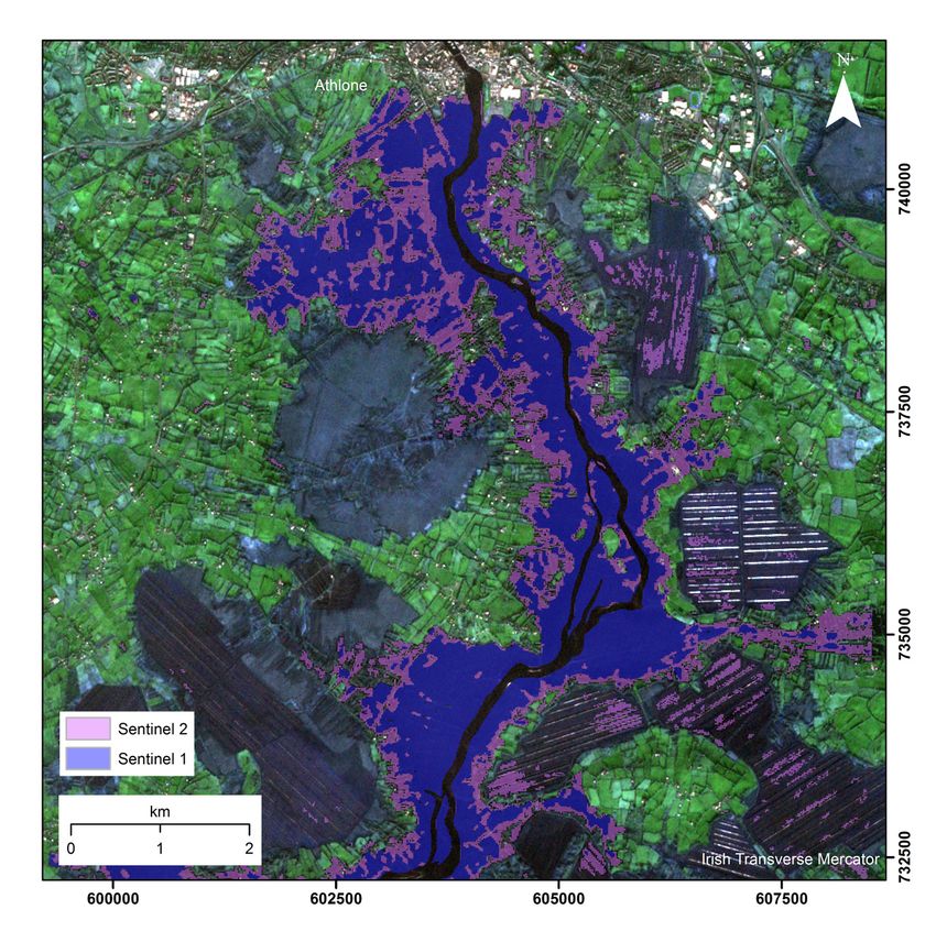
O’Hara et al.: Impact of winter floods 2015–2016

flooding and monitor recovery is well established (Rango              optical sensors, SAR can operate day or night, regardless of
and Solomonson, 1974; Profeti and MacIntosh, 1997; Joyce              atmospheric conditions (Gibson 2000). Interpreting RADAR
et al., 2009, Twele et al., 2016). Optical sensors (e.g. Sentinel     images is not as straightforward as for optical data. The
2, Landsat 8) map surface water based on the different                strength of the returned signal, measured as a backscattering
reflectance characteristics for soil, vegetation and water in         coefficient (sº), is a function of sensor specification
the visible, infrared spectrum. Reflectance-based mapping             (wavelength, polarisation and incidence angle), as well as
typically uses band combinations of near-infrared (NIR; ~0.7          environmental factors at the surface (roughness, geometry
mm–1.4 mm), shortwave infrared (SWIR; 1.4 mm–3 mm) and                and water content) (Campbell 2002). SAR flood mapping is
green (0.55 mm) light to record changes in flood extent (Ouma         usually undertaken at the X-band (3 cm wavelength), C-band
and Tateishi 2006, Ji et al., 2011; Du et al., 2016). Thermal         (5 cm wavelength) or L-band (23 cm wavelength). Longer
infrared images (8 mm–13 mm) may also be used (LeBlanc                wavelengths can penetrate deeper into thick vegetation
et al., 2014). The high thermal inertia (resistance to change in      canopy, although both X- and C-band SAR techniques have
water temperature) and emissivity of water appear as areas            demonstrated capability in mapping wetlands and regions
of homogeneous surface temperatures when flooded. The                 underlying a forest canopy (Lang and Kasischke, 2008).
potential of optical data for flood mapping is severely restricted    A surface is considered rough when it has dimensions
by vegetation canopies, a dependence on solar energy and              comparable to the incident wavelength. Smooth water
interference from clouds (Musa et al., 2015). Compositing             surfaces have low backscatter due to specular reflection and
daily images from high-temporal-resolution imagery (e.g.              appear very dark, while rougher land surfaces reflect more
Moderate Resolution Imaging Spectroradiometer [MODIS]                 energy and look brighter. Roughened water surfaces from
sensor aboard the Terra and Aqua satellites) can minimise             strong winds, precipitation, high-flow velocity or partially
cloud interference but at the loss of spatial resolution and          flooded vegetation appear in different levels of grey and
mapping accuracy (Chen et al., 2013). Unmanned aerial                 can be difficult to distinguish from land surfaces (Martinis
vehicles (UAVs) have been applied to flood mapping over               et al., 2015). In certain instances, surface water below the
small areas using high-resolution imagery (Feng et al. 2015).         canopy will increase backscatter relative to dry conditions
Multispectral images can observe the effect of stress on crops        due to increased signal reflectance (the double bounce effect)
(reduced photosynthesis production, stomata closure and               (Horritt et al., 2003).
decreased respiration; Carter and Miller, 1994), which can            SAR systems transmit and receive signals in single (horizontal
be used to infer prolonged soil waterlogging and to measure           [H] or vertical [V]) or dual polarisations (H and V), along the
vegetation recovery. In broadband sensors, these stresses are         geometric plane a RADAR pulse propagates. Four polarisation
typically characterised by reduced reflectance in the NIR region      combinations are possible (HH, HV, VH and VV), and all can
and increased reflection in red light. A normalised ratio of red      potentially be used for flood mapping. The HH (horizontal
and NIR bands, known as a normalised difference vegetation            transmit, horizontal receive) polarisation often displays the
index (NDVI), exploits this relationship to identify healthy and      highest contrast between water and land (Manjusree et al.,
senescent plants and is often used as a proxy for photosynthetic      2012). Sentinel 1 can collect HH polarisation, but it is not
activity and plants biomass (Pettorelli, 2014). NDVI is a unitless    systematically acquired over land surfaces (Sentinel 1 SAR
index ranging from –1 to 1; healthy vegetation has high positive      User Guide, https://sentinel.esa.int/web/sentinel/user-guides/
values, stressed vegetation has lower values, while bare soil         sentinel-1-sar). VV polarisation (vertical transmit, vertical
and water have values around or less than zero, respectively.         receive) data have generally been viewed as less capable than
Several studies have shown a correlation between wet soil             the HH data (Bourgeau-Chavez et al., 2001; Gstaiger et al.,
and NDVI values (Lozano-Garcia, 1991; Levine, 1994; Ciallela          2012), although VV polarisation has demonstrated superior
et al., 1997) and demonstrated crop response to inundation            ability in identifying partially submerged fields and features in
(Streyer et al., 2013; Džubáková et al., 2015) or other weather-      certain circumstances (Manjusree et al., 2012). Using Sentinel
based natural disasters (Rodgers et al. 2009; Fu et al. 2014).        1 imagery, Twele et al. (2016) reported high classification
Pantaleoni et al. (2007) used Landsat 5 Thematic Mapper NDVI          accuracy (>94%) using VV polarisation relative to that for VH,
images to quantify crop damage following severe flooding and          the latter having a greater misclassification rate in agricultural
the subsequent ponding of water on low-infiltration soils. A          lands. Clement et al. (2017) achieved similar accuracy (97%)
negative response was observed in difference images taken             mapping winter floods in the UK in 2015–2016. Their study
before and after submergence. NDVI differencing highlighted           highlighted the utility of Sentinel 1 in identifying pluvial flooding
inter-annual disparity caused by flood damage (Michener and           at distances from water bodies, as well as a strong correlation
Houhoulis, 1997).                                                     between Sentinel 1 and Sentinel 2 flood maps.
SAR is an active remote sensing technology that emits a               Flood extents are generally derived from SAR images using
RADAR pulse and measures returning backscatter. Unlike                a histogram-based, backscatter thresholding approach. This

                                                                                                                                            45
                                                       Bereitgestellt von St. Patrick's College, Maynooth University | Heruntergeladen 21.10.19 12:57 UTC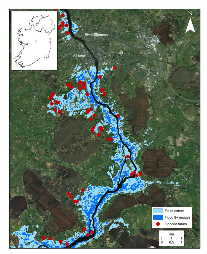
Irish Journal of Agricultural and Food Research

computationally fast and effective pixel-based method works             EMS) and optical (Sentinel 2) flood maps;
by splitting the histogram into “water” and “non-water” classes      5. To observe post-flood recovery in vegetation canopy using
based on a single backscatter value taken from the image                Landsat 8 NDVI images.
histogram (Di Baldassarre et al., 2011; Sahoo et al., 1988).
The threshold can be optimised using the Otsu algorithm or
                                                                     Materials and methods
through careful manual adjustment (Otsu 1979). Its major
limitation is that it provides a global threshold, which may
not be suitable in all areas of the image. Other methods of
segmentation include change detection (Brivio et al., 2002;          Satellite data
Wang, 2002; Martinis et al., 2011), image segmentation and           A total of 33 RADAR images were created from Sentinel 1A
clustering (Horritt, 1999; Mason et al., 2012), or a combination     backscatter data captured every 12 d from 19 November 2016
of these techniques (Martinis et al., 2009; Matgen et al.,           until 23 February 2016, and intermittingly after that, on 30
2011). Others have proposed artificial neural networks               March and 11 April. Data were downloaded from ESA’s Sentinel
(Kussul et al., 2008) or support vector machines (Insom              Scientific Data Hub (SciHub; https://scihub.copernicus.eu).
et al., 2015) for supervised classification of SAR images.           The selected imagery provided almost national coverage.
Long et al. (2014) and Clement et al. (2017) have defined            Two narrow strips of land along the eastern and western
thresholds based on image differencing between wet and dry           coasts, which lay outside the chosen image swaths, were
periods, where regions with the greatest negative change in          omitted from the study to reduce processing time. RADAR
backscatter were classified as inundated. Huang et al. (2017)        scenes are available for these areas. The area of land in the
have proposed a threshold based on terrain indices derived           omitted swaths is relatively small and predominantly coastal
from coarse-resolution digital elevation models (DEMs), as a         or mountainous. They were considered unlikely to contain
way of defining surface water and shadow effects.                    regions of flooding pertinent to this study. Data specifications
Flood depth and volume can be estimated by combining                 for the Sentinel missions are provided in Table 1. To allow
RADAR imagery with DEMs to determine the elevation of the            a comparison with currently available RADAR flood maps,
land–water interface (Puech and Raclot, 2002; Matgen et al.,         Copernicus EMS flood maps (EMS rapid mapping [EMSR];
2007). Water height extraction at coarse (~30 m) spatial             EMSR149) for an area surrounding Athlone, Westmeath (13
resolution is possible (LeFavour and Alsdorf, 2005; Kiel et al.,     December 2015) were downloaded from the Copernicus EMS
2006); however, such DEMs are generally associated with low          website (http://emergency.copernicus.eu/mapping).
vertical accuracy and are unsuited to terrain or hydrological        Multispectral imagery (21 December 2015) from Sentinel 2A
modelling (Li and Wong, 2010). At coarse resolution, the loss        was also downloaded from SciHub to allow a comparison
of definition of fine-scale topographic information (e.g. river      with Sentinel 1 flood maps. These were downloaded as top-
embankments, hedges and walls, ditches, etc.) through pixel          of-atmosphere (TOA) products (Level 1C) and converted to
aggregation can lead to overprediction of flood extents and          surface reflectance using a dark-object subtraction algorithm
depth (Sanders, 2007; Cook and Merwade, 2009). High-                 (Chavez, 1996) in the Semi-Automatic Classification plugin
resolution elevation data from laser scanning (light detection       (v.5.2.2) in the geographic information system software QGIS
and ranging [LIDAR]) and aerial photogrammetry can more              (v.14.2). Satellite images require several stages of processing
accurately model topographical surfaces and improve                  to geometrically and radiometrically correct raw data. TOA
estimates of flood extent and depth (Charlton et al., 2003;          data have higher reflectance values as the dataset includes
Coveney and Roberts, 2017).                                          scattered light reflecting off atmospheric particles (dust,
In response to extensive flooding in winter 2015–2016, the           molecules and water vapour), as well as cloud and cloud
goal of this pilot study was to investigate the feasibility of       shadow on the surface. These can be a source of error in earth
extending RADAR mapping coverage for the Republic of                 observation studies and need to be eliminated or minimised to
Ireland using Sentinel 1 backscatter data. The objectives of         provide actual surface reflectance values.
the study were as follows:                                           To demonstrate the effect of persistent flooding on pasture
1. To create flood maps at regular intervals to monitor the         yields the following spring, a mosaic of 18 NDVI images from
   development of flooding at a national scale, with a focus         April and May 2016 covering the Border, Midland and Western
   on rural areas;                                                   regions were compiled from United States Geological Survey
2. To determine the worst-affected areas and identify areas of      (USGS) Landsat 8 scenes. Mosaics were created for flood
   persistent flooding;                                              (spring 2016) and non-flood (spring 2015) years. NDVI
3. To estimate flood depth and volume;                              images were created using the established equation (NIR
4. To assess the accuracy of the produced map against               – red)/(NIR + red) (Tucker 1979). Landsat was preferred to
   ground truth, as well as in relation to RADAR (Copernicus         Sentinel 2 because of its extensive image archive, which

46
                                                      Bereitgestellt von St. Patrick's College, Maynooth University | Heruntergeladen 21.10.19 12:57 UTC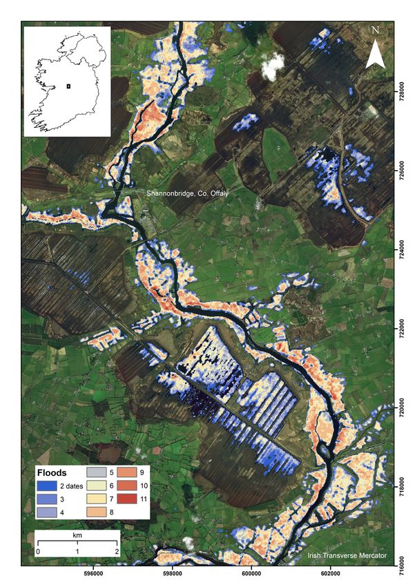
O’Hara et al.: Impact of winter floods 2015–2016

                                       Table 1. Data specifications for the Sentinel satellites
                                                 Sentinel 1A                                                Sentinel 2A

 Frequency/wavelength                         C-band (5.4 GHz)                                    0.443 mm–2.150 mm (VIS–SWIR)

 Orbit                                    693 km (sun-synchronous)                                   786 km (sun-synchronous)

 Interval                                           12 d                                                        10 d

 Acquisition dates                               19 Nov. 2015                                               21 Dec. 2015
                                             1, 13, 25 Dec. 2015
                                             6, 18, 30 Jan. 2016
                                              11, 23 Feb. 2016
                                                 30 Mar. 2016
                                                 11 Apr. 2016
 Mode                                     Interferometric wide swath                                     Multispectral imager

 Swath width                                       250 km                                                      290 km

 Product                                Level-1 ground range detection                         Level-1C top of atmosphere reflectance

 Spatial resolution                                 10 m                                                     10 m, 20 m

 Polarisation                                     VV + VH                                                         -

 % cloud cover                                        -                                                          3%

covered the duration of the study period. TOA images                   maxima and topographic depressions, which can overpredict
were downloaded from the USGS website (Earth Explorer;                 flood area (Brandt 2005; Zandbergen 2006). Monte Carlo
https:/earthexplorer.usgs.gov). Masking of cloud and cloud             simulations have been widely applied to DEM to quantify
shadow was accomplished using the F-mask algorithm (Zhu                error propagation from positional uncertainty (Heuvelink
et al., 2015) and converted to surface reflectance using the           et al., 1989; Wechsler and Kroll, 2006; Zandbergen, 2011;
Landsat Ecosystem Disturbance Adaptive Processing System               Leon et al., 2014). They have been used in flood and surface
(LEDAPS) algorithm (Schmidt et al., 2013). NDVI values,                hydrological modelling (Wu et al., 2008; Domeneghetti et al.,
based on mean pixel values within a 25 m radius, were                  2013; Bodoque et al., 2016). A Monte Carlo simulation of
extracted at ~4,000 randomly selected locations.                       500 perturbed DEMs was created, which included a random
Existing water bodies (rivers and lakes) were extracted from           error term drawn from the original root mean square error
Ordnance Survey Ireland (OSI) vector data and used to mask             (RMSE). These were produced in geographic information
the normal extent of surface water. This mask included the             system software ArcGIS using the methodology proposed
locations of 128 turloughs, seasonally flooded wetlands in             by Zandbergen (2011). Errors were normally distributed and
karst regions, which were obtained from the Environmental              spatially autocorrelated based on a five-cell neighbourhood
Protection Agency (EPA) (Johnston, Turlough Database).                 (50 m). The modified DEM was resampled to 10 m (ArcGIS)
Hydrograph data for river gauge stations were obtained                 using bilinear interpolation to match the spatial resolution of
from the OPW. Daily average river heights were extracted               Sentinel 1. Maximum elevation heights beneath individual
from 10 stations within the River Shannon catchment. Daily             flood regions were extracted from the modified DEMs using a
precipitation data were downloaded from the meteorological             zonal statistics algorithm (ArcGIS), which calculates summary
service for 391 stations distributed across the country. Daily         statistics on raster values based on zones within another
values were aggregated to give mean rainfall values. Land              dataset. The maximum DEM elevation value below each zone
cover data were extracted from the 25 ha Coordination of               was assumed to represent the maximum height reached by
Information on the Environment (CORINE) database, available            the flood waters. The difference between the DEM elevation
at the EPA. Soil and subsoil information was available through         and this maximum value permitted a pixel-by-pixel estimate
the Teagasc Soils and Subsoils database (Fealy et al., 2009).          of flood depth (in metres), which was converted to volume by
This subsoil map had a nominal working scale of 1:50,000 and           multiplying by the pixel area.
included a classification of soils into poor and well drained.
A 20 m spatial resolution DEM (± 2.5 m vertical error) from            Flood mapping procedure
the OSI was used to estimate flood depth and volume.                   Map creation followed the recommended practice
DEM resolution and accuracy have a significant impact on               published by the United Nations Space-based Information
water surface elevations and flood extent (Darnell et al.,             for Disaster Management and Emergency Response (UN-
2008; Fisher and Tate, 2006). The averaging of elevation               SPIDER) portal (UN-SPIDER Knowledge Portal 2016). The
values within coarse footprints can subdue local elevation             image processing workflow was executed through ESA’s

                                                                                                                                           47
                                                      Bereitgestellt von St. Patrick's College, Maynooth University | Heruntergeladen 21.10.19 12:57 UTC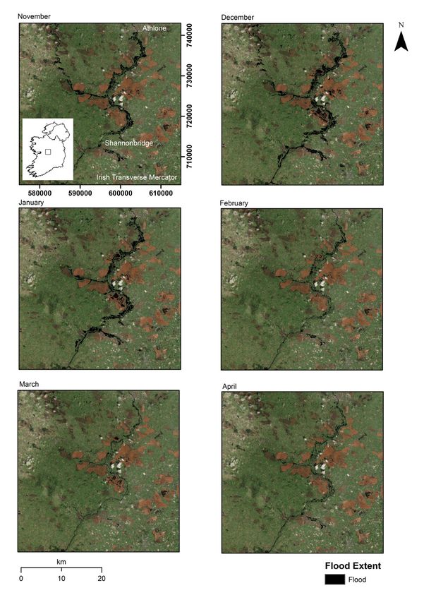
Irish Journal of Agricultural and Food Research

Sentinel Application Platform, SNAP (v.4.0), following a                speckle follows a Gaussian distribution and replaces central
step-by-step procedure of calibration, filtering, masking               pixels within a 7 × 7 pixel moving window with the average
and rectification. The subsequent analysis used ArcGIS                  of all values that fall within 2 s.d. (Lee, 1983). A backscatter
(v.10.2.2), QGIS and R statistical software (v.3.2.3). The              value for flood water was manually determined for each of the
map (Figure 1) is available as a download (raster format)               33 scenes through visual inspection of the image histograms.
from the Teagasc data repository T-stór (www.t-stor.                    Each histogram typically displayed a bimodal or multimodal
teagasc.ie) and through the ArcGIS Online portal (www.                  distribution. Low backscatter values corresponded to flat
esri.com). Displayed projection coordinates are Irish                   water (including noise) and high values corresponded to non-
Transverse Mercator (European Petroleum Survey Group                    water classes, allowing a binary segmentation on the images
[EPSG] code 2157).                                                      into water or non-water pixels. A mean threshold was defined
                                                                        for each image from backscatter values recorded at known
                                                                        surface water locations. Images were then transformed from
                                                                        internal sensor geometry to a projected coordinate reference
                                                                        system (World Geodetic System [WGS] 1984) using inherent
                                                                        ground control references and National Aeronautics and
                                                                        Space Administration (NASA)’s Shuttle RADAR Topography
                                                                        Mission (SRTM) Global 3 arc-second DEM. Individual scene
                                                                        masks were mosaicked into one image for each acquisition
                                                                        date in ArcGIS. To reduce potential misclassification arising
                                                                        from erroneous threshold definition and uncorrected speckle
                                                                        effect, isolated single-pixel flooded areas (0.01 ha) and pixels
                                                                        classified as inundated on just one occasion were excluded
                                                                        from analysis (24,166 ha in total).

                                                                        Noise removal
                                                                        Thresholding invariably misclassifies pixels at the class
                                                                        boundary due to the binary nature of the thresholding
                                                                        process. Regardless of the method used, thresholding
                                                                        uses a single point to separate pixels. This creates noise,
                                                                        which must be reduced. Noise in this study is defined as
                                                                        low backscatter values not associated with flooding. The
                                                                        principal sources of noise included topographic shadow
                                                                        (where slopes in the opposite direction of image acquisition
                                                                        are observed with very low or zero backscatter), estuaries
                                                                        and beaches (which appeared as water or not, depending
                                                                        on the tidal regime); flat constructed surfaces (e.g. car
                                                                        parks, extensive flat roofs, airport runways); and anomalies
                                                                        created during processing (banding along the swath’s
                                                                        edges and merged boundaries). Most scene- and sensor-
                                                                        related noise was masked using a summer RADAR image
                                                                        by identifying normally occurring low-backscatter regions. A
Figure 1. Estimated extent of flooding in the winter of 2015–2016       slope mask filtered out surface gradients greater than 5°,
(areas >0.01 ha and flooded on >1 occasion).                            which could cause shadowing. Masking turloughs entirely
                                                                        was challenging and, hence, these remained a source of
The initial step created a calibrated backscatter image (10             unknown error within the final map. These are low-lying
m × 10 m pixel) in decibels (dB) in VV polarisation. These              areas of limestone geology, which become flooded in wet
images contain inherent speckle, which is the random                    weather through the rising of groundwater. Defining a fixed
granular noise in SAR images caused by heterogeneous                    boundary for these wetlands is difficult as water levels are
scattering surfaces within a pixel. Speckle changes scene               dynamic. The weather on the date of acquisition is a further
backscatter values, which can hinder accurate image                     source of noise. Surface waters roughened by high-velocity
segmentation and classification (Mansourpour et al., 2006).             flow, rainfall and speedy winds during acquisition may not
It was removed using a Lee-Sigma filter, which assumes that             appear smooth with C-band SAR.

48
                                                         Bereitgestellt von St. Patrick's College, Maynooth University | Heruntergeladen 21.10.19 12:57 UTC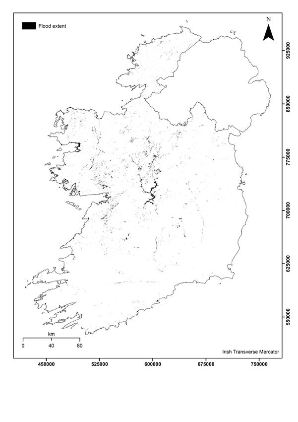
O’Hara et al.: Impact of winter floods 2015–2016

Results                                                                  they were classified as flooded. Most of the region depicted
                                                                         in this figure was inundated for a period between six and nine
                                                                         acquisition dates. Smaller areas were flooded in this figure for
Extent                                                                   the entire period of the study.
The final flooded area (Figure 1) on each acquisition was
calculated as the summed area of pixels remaining after                   Table 3. Number of times a pixel was classified as flooded, indicat-
                                                                                        ing the extent of persistent flooding
noise removal. The calculated area was 24,356 ha, which
is greater than the combined surface area of Loughs Ree                   Number of times flooded        Area (ha)

and Derg (22,300 ha), two lakes on the River Shannon. To                  1                                  22,160
account for the 7 m positional inaccuracy (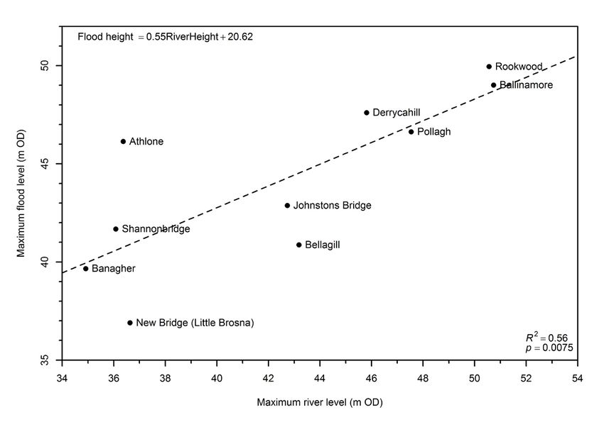
Irish Journal of Agricultural and Food Research

Figure 2. Flood extent at Shannonbridge, Offaly (November 2015–April 2016).

1 d rainfall (P = 0.217), with an adjusted R2 of 0.07. Results        inundated land mapped by Sentinel 1. The remaining ~13%
from models with rainfall for 4 d and 6 d (P = 0.13 and P =           was made up of several categories of land cover (e.g. marine
0.22, respectively). Beyond 6 d, significant effects were found       and inland waterways, beaches, quarries etc.).
at each interval; however, the explanatory power of these
models was weaker compared with the model for 5 d rainfall            Depth/volume
(Figure 4).                                                           Using mean flood heights derived from the Monte Carlo
The majority of affected soils were alluvial or lacustrine (8,100     simulations, flood volumes were estimated at 528,863,333 m3
ha, or 33% of the flooded area), cut-over peat (7,000 ha, 28%)        (95% confidence interval: 482,078,000 m3, 575,648,500 m3).
or poorly drained soils (1,500 ha, 6%). However, approximately        In comparison, Lough Ree, the second largest lake on the
3,000 ha (13%) was previously classified as “well drained”            River Shannon, has an estimated volume of ~650,000,000 m3.
(mainly brown earths and brown podzols; Fealy et al. 2009).           To further determine the error distribution of the estimated
A large proportion of flooded land (~61%) was agricultural,           flood depth, a further 2,500 Monte Carlo simulations were
of which ~50% was pasture, with an additional 11% in areas            run on a subset region using the “spup” package (v.0.1-1) in
principally dominated by agriculture but with significant natural     R. Confidence intervals around the estimated mean values
vegetation also. The area of arable and forested land affected        decreased with increasing number of simulations (Figure 5).
was negligible (each
O’Hara et al.: Impact of winter floods 2015–2016

Figure 3. Persistence of flooding at Shannonbridge, Offaly. Each colour represents the number of times a pixel was classified as flooded.

Figure 4. Flood extent vs. rainfall in the previous 5 d.

                                                                                                                                               51
                                                          Bereitgestellt von St. Patrick's College, Maynooth University | Heruntergeladen 21.10.19 12:57 UTC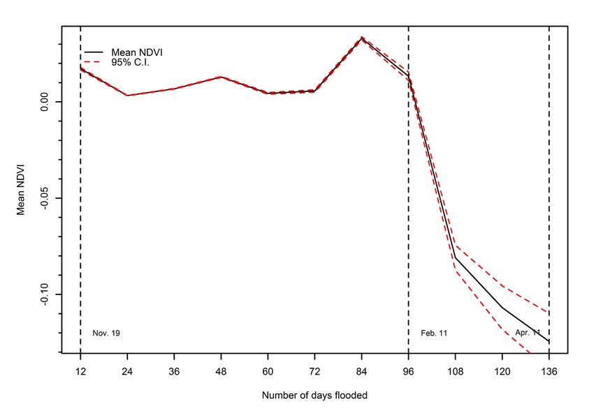
Irish Journal of Agricultural and Food Research

Figure 5. Example of variable mean and 95% confidence intervals for flood depth at a sample location with increased Monte
Carlo simulations.

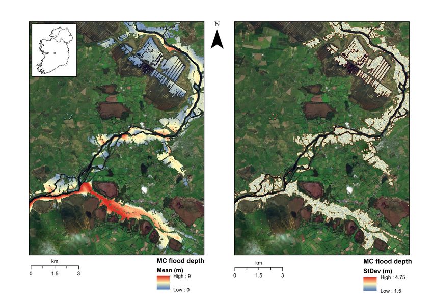
depths generated using this modified DEM are illustrated in          aerial imagery. When areas flooded only once were included,
Figure 6. As expected, areas closest to river channels are           the number of flooded agricultural buildings was 35 of 125
deeper, and depth decreases with Euclidean distance from             (28%). The remaining structures were predominantly rural
the channel. Standard deviations for each pixel illustrate           domestic properties (many in coastal locations), riverside and
the error range present within a small and topographically           lakeside buildings (sheds, boat houses) and structures within
homogeneous area. Histograms for four randomly selected              sports facilities and industrial/transport sites.
points further illustrate the error distribution for depths at       The effect on crops may not have been immediately evident.
these grid cells. Mean flood depths vary by location. However,       Mean NDVI values for pastures within the flooded area the
the s.d. across the subset region is approximately 1.95 m.           following spring 2016 was 0.70 (s.d.: 0.18). By comparison, in
                                                                     the same period, mean NDVI values for non-flooded grassland
Damage to farms                                                      on poorly drained and well-drained soils were 0.78 (s.d.: 0.11)
Teagasc farm advisors nationwide conveyed damage reports             and 0.80 (s.d.: 0.12), respectively. A non-parametric Kruskal–
from affected farmers, including lost bales of hay or silage,        Wallis rank sum test carried out using the “stats” (v.3.4.1), and
drowned animals and flooded buildings and yards (Teagasc,            “dunn.test” packages (v.1.3.4) in R found that flooding had
personal communication). A greater proportion of the                 a significant effect on grassland NDVI values the following
buildings flooded on >1 occasion were agricultural buildings.        spring (P-value < 0.001). Pairwise multiple comparisons
Intersecting the map with building location data from the OSI,       showed no evidence for different median NDVI values during
13 of 24 buildings (54%) identified as within the national flood     the first eight events. There were significant differences in
extent could be classified as agricultural in high-resolution        NDVI values for flood events numbering between eight and

52
                                                      Bereitgestellt von St. Patrick's College, Maynooth University | Heruntergeladen 21.10.19 12:57 UTC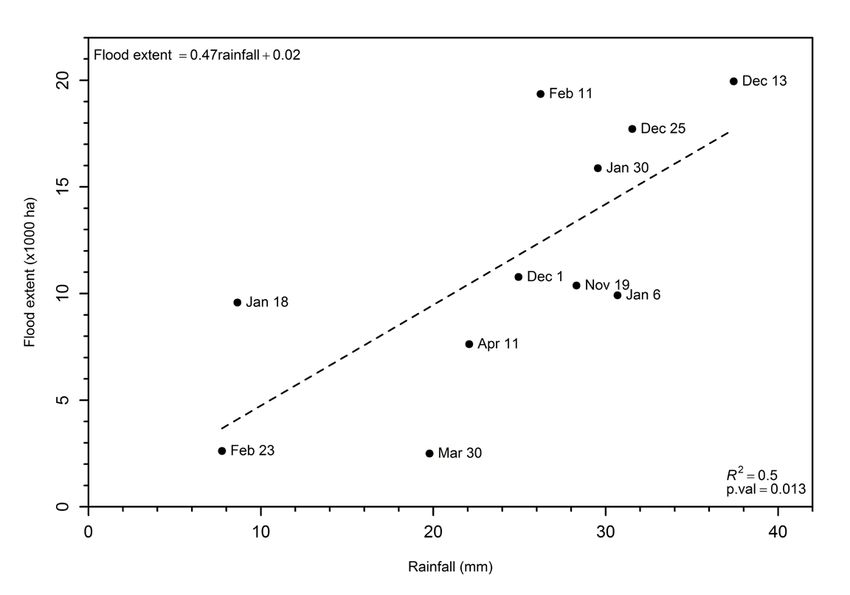
O’Hara et al.: Impact of winter floods 2015–2016

Figure 6. Mean and s.d. of estimated flood depths at Athlone, Westmeath. Depth uncertainty is shown as the error distribution histograms at
four randomly selected points.

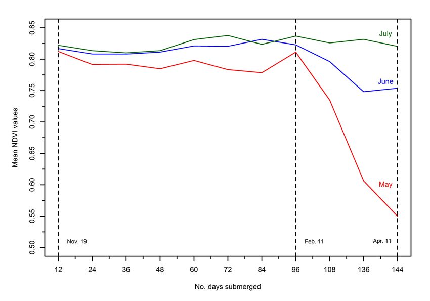
Figure 7. Mean NDVI values for flooded pasture (April/May 2016) as a function of flood duration. Values are based on mean NDVI values
within 25 m of sample locations (n = 4,000).

nine (P-value < 0.001) and between nine and 10 (P-value                 Validation
< 0.001) (Figure 7). An inter-annual comparison between                 The map was validated against three independent sources:
NDVI values in 2016 and 2015 showed a similar trend with                1. R
                                                                            eports of flooded fields from individual farmers;
no significant differences between the years until after eight          2. F
                                                                            lood map created from Sentinel 2 optical data of Athlone,
flood events (Figure 8). Spring 2015 weather conditions were               Westmeath;
typical, with air temperatures at or marginally lower than LTAs.        3. C
                                                                            opernicus EMS flood map (EMSR149) of Athlone,
Growing conditions may have been depressed in certain areas                Westmeath.
as a result of the above-average rainfall, which was heavy in           Reports of flooded farms directed to Teagasc advisors
places (Met Éireann, 2015).                                             provided a direct means of validating the map. A database

                                                                                                                                              53
                                                         Bereitgestellt von St. Patrick's College, Maynooth University | Heruntergeladen 21.10.19 12:57 UTC
Irish Journal of Agricultural and Food Research
Figure 8. Difference in NDVI values between spring 2015 and spring 2016 for flooded pasture. Values are based on mean NDVI values within
25 m of sample locations (n = 5,422).
of 57 farms that reported flood damage was overlaid with the bands (commonly called a normalised difference water index,
estimated extents. Accordingly, 49 farms intersected the flood NDWI) (McFeeters, 1996) was used to map the floods for a
boundary, an 86% agreement between field and satellite data. region of interest south of Athlone, Westmeath. The green
There was no way of identifying Type 1 errors (false positives) shaded area in Figure 10 shows the inundated area seen by
among these reports, as only flooded properties were listed. Sentinel 2 on 21 December, and the blue shaded area is the
The mean inundated area on these farms was ~3 ha, with flood extent obtained from Sentinel 1 on 25 December. There
the area maximum flooded for any one farm reaching 176 ha. was a 58% overlap between these maps within this region of
Most flooded farms were immediately adjacent to the River interest. The disparity is probably due to a 4-d separation in
Shannon. Moreover, 55 flooded fields were >500 m from a overpasses, as well as concomitant changes in water levels
water body, emphasising the extensive reach of flood waters over this period. It is also worth noting that during the Sentinel
and the role of pluvial flooding in the overall flood magnitude. 1 overpass, weather stations recorded 17 mm of rain that
Flooded farms in the Shannonbridge/Athlone areas are day (more than the LTA for December), with a wind speed of
illustrated in Figure 9. approximately 4 m/s gusting to 11 m/s. These conditions could
Clear skies across the Midlands on the morning of 21 have sufficiently roughened the water surface to increase
December (3% cloud cover) allowed Sentinel 2 to capture backscatter above the defined threshold values.
surface reflectance. This facilitated a comparison of optical The final validation of the flood extent was a comparison with
and microwave methods of map creation at the same spatial the Copernicus EMS map. Maps from 13 December were
resolution (10 m). A normalised difference of green and SWIR compared with Sentinel 1 maps from 25 December using an
54
Bereitgestellt von St. Patrick's College, Maynooth University | Heruntergeladen 21.10.19 12:57 UTCO’Hara et al.: Impact of winter floods 2015–2016
Figure 9. Farms reporting floods in the environs of Athlone, Westmeath. Areas flooded on >8 dates are coloured dark blue.
Figure 10. Comparison of flood maps from Sentinel 1 (25th December) and Sentinel 2 (21st December) imagery. Base map is an ESA Sen-
tinel 2 red, green and blue (RGB) image at 10 m resolution.
55
Bereitgestellt von St. Patrick's College, Maynooth University | Heruntergeladen 21.10.19 12:57 UTCIrish Journal of Agricultural and Food Research
error matrix (Congalton and Green, 2008). As Copernicus At two locations, flood maxima were within 25 cm of the
draws data from a number of sensors and polarisations, it measured river heights. The largest difference was at the
was assumed to have greater accuracy. The Sentinel map Athlone station, where flood levels were overestimated by
showed good agreement to Copernicus data, with 79.5% of 9.70 m. A Grubbs outlier test conducted using the “outliers”
pixels matching (Table 5). Local meteorological conditions package in R (v.0.41) identified Athlone as a probable outlier
on 13 December were mild (3 mm rainfall, speed 4 m/s (G = 2.09, U = 0.45, P = 0.075). Removing this station from
gusting to 10 m/s), so weather conditions are unlikely to the linear model increased the correlation to 0.85 (P = 0.006)
be responsible for the difference in classification. Low user and improved the R2 value of the fitted model to 0.8 (P <
accuracy of the Sentinel 1 data for flooded areas (66%) 0.001).
probably reflected the reduced ability of the C-band sensor
to resolve flooding in the presence of canopy vegetation. It
Discussion
may also reflect actual differences in flood height on different
acquisition dates. Copernicus EMS maps are compiled from
multiple sensors at different wavelengths and polarisations.
This improves the detection accuracy of Copernicus relative Flood extent
to single-wavelength and single-polarisation maps. Although Flooding is a common occurrence in Ireland, particularly in
the imagery was acquired on different days, combining both the Midlands, where the low gradient and poor flow capacity
Sentinel 1 and Sentinel 2 images improved classification of many rivers lead to floods under typical winter weather
agreement (91%; Table 6), underlining the complementary (Charlton et al., 2006). Many Irish soils have a natural
nature of the two Sentinel missions and emphasising the disposition towards saturation during winter months, or at any
potential of Sentinel 2 data for both flood classification and time under heavy rain, allowing surface ponding to develop.
map validation. In this instance, Sentinel 2 was better able to While there is an increase in the number of severe floods
define flood extent based on apparent differences in NDWI across Europe (Kundzewicz et al., 2013), flooding of the
values between flooded and non-flooded pixels. magnitude witnessed in winter 2015–2016 remains unusual
Estimated flood depths were validated against a time series in Ireland. A long-term, upward trend in the annual number
of river heights maintained by the OPW for the Shannon River of rain days and volume of precipitation will, however, likely
Basin District (SRDB). Maximum river levels were recorded see higher flood risk in the future (Kiely et al., 2009). In a
for 10 monitoring locations in the Shannon catchment, where study of future climate scenarios in terms of water supply and
flooding was recorded within a 500 m radius. Ordinary least flooding, Charlton et al. (2006) predicted a probable increase
squares linear regression was used to predict flood extent in the magnitude and frequency of winter floods in the western
based on river gauge data. A significant relationship was half of Ireland before the end of this century in response to
found (P = 0.007), with an adjusted R2 of 0.56 (Figure 11). increased surface runoff.
Table 5. Accuracy assessment of Sentinel 1 flood map versus Copernicus EMS data
Sentinel 1 flood map
No flood Flood Total User accuracy.
Copernicus EMS
No flood 37 1 38 97.4%
Flood 17 33 50 66.0%
Total 54 34 88
Producer accuracy. 68.5% 97.1% Overall accuracy 79.5%
Table 6. Accuracy assessment of combined Sentinel 1 and Sentinel 2 maps versus Copernicus EMS data
Combined Sentinel 1 and Sentinel 2 flood maps
No flood Flood Total User accuracy
Copernicus EMS
No flood 31 7 38 81.6%
Flood 1 49 50 98.0%
Total 32 56 88
Producer accuracy 96.9% 87.5% Overall accuracy 91.0%
56
Bereitgestellt von St. Patrick's College, Maynooth University | Heruntergeladen 21.10.19 12:57 UTCO’Hara et al.: Impact of winter floods 2015–2016 Figure 11. Relationship between estimated maximum flood levels and maximum river heights at 10 monitoring stations across the Shannon catchment. Flood heights are based on mean elevation values within 500 m of each station. Athlone is identified as an outlier (see text). Approximately 24,356 ha were inundated between 19 (Manjusree et al., 2012). Additional bands can allow more November 2015 and 11 April 2016. Where misclassification accurate segmentation of each scene. The thresholding errors were noted, they were predominantly from specular method used in the paper was based on manually adjusting surfaces (e.g. airport runways, parking facilities and flat roofs) histograms to an appropriate grey level (Di Baldassarre et al., not removed by the masking process, although, in some 2011). This method is widely used, fast and computationally instances, these could reflect actual cases of surface water. efficient, but it is also labour intensive when the number Higher accuracy in flood delineation would be expected had of scenes is large. Twele et al. (2016) presented a fully both Sentinel satellites been available at the time. Using both automated processing chain designed for Sentinel flood polarisations could also have increased accuracy (Twele detection and monitoring in near-real time (
Irish Journal of Agricultural and Food Research

1984), and the flood extent had a significant response to                 poor penetration of the canopy due to the C-band and VV
total rainfall depth over several preceding days. The best                polarisation used (Townsend, 2002). Longer wavelengths
explanatory model for flood extent was that for 5 d rainfall,             (L-band) and HH polarisation provide greater penetration into
which explained 51% of the variance in flood extent. In the               forest canopies (Wang et al., 1995). It may also reflect a mostly
short term, this likely reflects the rapid expansion of floods            upland distribution of Irish forests (Upton et al., 2014), where
where rain was unable to infiltrate saturated or flooded soils.           extensive flooding would be unlikely to occur. Poor delineation
The continued significant effect over a more extended period              in urban areas is generally a result of RADAR shadow caused
may reflect the slow retreat of waters once an area was                   by high buildings. These are areas that cannot be detected
flooded (see Figure 2). Unusually high rainfall over the winter           as the RADAR pulse is either obstructed from reaching them
period maintained flood extents longer than would be normally             or reflected away (e.g. off flat or sloping surfaces, such as
expected. When soils are at field capacity or saturation, any             roofs). Flood mapping of urban environments requires higher-
further precipitation will lead to increased surface runoff.              resolution SAR and elevation data (Mason et al., 2012;
Infiltration-excess overland flow is triggered when the rainfall          Brown et al., 2016). This study concentrated on rural areas
rate exceeds the infiltration capacity of a soil. It is rare but          and did not seek to identify flooding in urban/forested regions
not unknown on Irish soils (Schulte et al., 2006), where it               specifically. Floods on areas of cut-over peat accounted for
can happen at any time during the year (Doody et al., 2010).              ~7,000 ha, which before reclamation, would have acted as
The risk is higher in winter, when the water infiltration rates           hydrological sinks for excess surface water.
can be as low as of 6.9 × 10⁻⁸ m/s (6 mm/d) on some soils
(Diamond and Shanley, 2003). An example infiltration-excess               Flood map uncertainty
pluvial flooding may be seen following intense rain over a                DEM uncertainty increases error propagation in hydrological
24-h period on 10–11 April (Met Éireann 2016c): 31–58 mm                  and topographical modelling (Casas et al., 2006; Fisher and
rain fell in 24 h in parts of the southwest, while stations in            Tate, 2006; Weschler, 2007). Cook and Merwade (2009)
Dublin reported their wettest day in half a century. This rainfall        demonstrated how flood inundation area was reduced
was immediately reflected in a three-fold increase in flood               with improved and increased resolution and accuracy in
area from 2,500 ha on 30 March to 7,600 ha flood on 11 April.             topographic data. To better quantify the vertical error that the
Saturation-excess overland flow occurs when the rain falling              DEM had on our estimates of depth and volume, a Monte
onto saturated areas does not have a chance to infiltrate due             Carlo simulation was used to estimate pixel-wise uncertainty
to rising groundwater or the discharge of lateral subsurface              across the map. Flood volume was determined with 95%
flow, and runoff is initiated (Davie, 2008). Saturation-excess            certainty to be between 482,078,000 m3 and 575,648,500 m3.
overland flow is mainly independent of rainfall intensity;                Estimate accuracy would have been considerably improved
instead, it is a factor of total rainfall and the soil and topographic    using a DEM with higher spatial resolution and a lower RMSE
factors. Areas prone to saturation expand and contract over               (from LIDAR and aerial photogrammetry), as demonstrated
different time scales as soil wetness increases (Hewlett and              in several studies (Charlton et al., 2003; Lane et al., 2003;
Hibbert 1967; Walter et al. 2000). This is the dominant type of           Mason et al., 2007; Schumann et al., 2009; Coveney and
overland flow generated under Irish conditions (Tunney et al.,            Roberts, 2017).
2000). Pluvial flooding would have contributed to the flooding
extent throughout the period. We can observe its impact                   Measuring post-flood recovery
on the 13 February map, when a steady period of flood                     In many areas of the world, flooding, and the excessive soil
contraction in January 2016 was reversed by persistent rain               moisture that accompanies it, can be a significant constraint
over several days. The result was a flood covering ~19,357               on agricultural productivity (Schulte et al., 2012). Persistent
ha, only marginally smaller than the post-Storm Desmond                   waterlogging presents several challenges for farmers after
maximum in mid-December. Other factors beyond rainfall                    surface waters subside. Excessive moisture can result in a
likely contributed to the flood extent. At catchment scale, this          collapse of soil aggregates (Hillel, 1998), and the subsequent
may be drainage density (Schottler et al., 2014) or the level             loss of trafficability can harm farm operations (Vero et al.,
of arterial drainage (Harrigan et al., 2014). At smaller scales,          2014). The elimination of air pores creates hypoxic conditions
flood persistence may reflect either differences in soil texture          in the root zone, which is detrimental to plant health (Jackson
or the presence and design of artificial drainage systems                 and Colmer 2005). Studies have found a reduction in
(Wiskow and van der Ploeg, 2007).                                         growth, leaf extension rate and chlorophyll concentrations of
Using the CORINE dataset, the greatest impact was on                      perennial ryegrass (Lolium perenne L.) following short-term
agricultural land, primarily grassland, which accounted for               waterlogging and submergence. For example, reduction in
~50% of the flooded area. Both forestry and urban regions                 plant biomass was demonstrated by McFarland et al. (2003)
constituted
O’Hara et al.: Impact of winter floods 2015–2016

were reduced by up to 70% and photosynthesis was reduced              an overall flood classification accuracy of 96% using a fusion
by 30%–50%.                                                           of data from SAR (COSMO-SkyMed) and multispectral images
Our findings indicated that the spring NDVI value for flooded         (RapidEye). For many areas, excessive cloud cover will limit
pasture was lower when measured against non-flooded                   the potential of optical data for flood mapping and damage
areas. NDVI values were only significantly different after the        assessment. Adopting a multisensor integration approach
period of submergence exceeded eight flood events (96 d).             increases the likelihood of imaging flood extent when cloud
There was no statistical difference in NDVI values for pixels         contamination is low; however, there are integration issues
flooded once up to eight times. After nine flood events (108 d),      between Landsat 8 and Sentinel 2 regarding differences in
a significant decrease in NDVI value was recorded during              spectral bandwidth, which can affect data fusion (Mandanici
the preceding period. This decline continued in subsequent            and Bitelli, 2016; Flood, 2017).
days, with NDVI value after 10 flood events (120 d) becoming          When carried out initially, this study was the first national
significantly lower again. This suggests that short-term              flood map prepared for Ireland using Sentinel 1 SAR.
waterlogging had little impact on spring NDVI. As flood               Sentinel provides an opportunity to monitor surface water and
duration increased, so too did the likelihood of flooding in late     inundation levels at weekly intervals nationally. Flood maps
winter and early spring (February and early March). As the            have been developed in the past over smaller areas. For
Sentinel 2 mission continues, its enhanced spectral resolution        example, in response to flooding in 2009, Service Régional
compared to Landsat 8 will be invaluable in monitoring post-          de Traitement d’Image et de Télédétection (SERTIT) mapped
event vegetation recovery. Sentinel 2 has three additional            the Shannon catchment as part of the Strategies and Actions
bands between 0.7 mm and 0.8 mm capable of detecting                  for Flood Emergency Risk Management (SAFER) programme
small changes in plant chlorophyll production (Delegido et al.,       (http://sertit.u-strasbg.fr/SITE_RMS/2009/18_rms_
2011). At local scales (
Irish Journal of Agricultural and Food Research

make use of both VV and VH polarisation. Greater automation          Conclusions
will be required, and the approach of Twele et al. (2016) is
promising. High-resolution topographic data will be essential        Sentinel 1 SAR images have been used to map the 2015–2016
to quantify flood depths and volumes accurately. The national        winter floods in the Republic of Ireland. Map accuracy was
mapping agency (OSI) is currently (summer 2017) laser                validated against three independent sources (farm reports,
scanning 185,000 ha nationally at high point density (https://       optical flood map and RADAR flood map). There was 86%
www.osi.ie/products/bluesky-aerial-imagery-lidar/bluesky-            agreement between the reported flooding and farm reports.
ireland). These elevation models will facilitate more accurate       Lower accuracy between different satellite-derived flood
flood modelling. For national-scale modelling, however,              maps probably reflected actual differences in flood height
the financial cost of acquiring high-resolution data can be          on different acquisition dates and under different weather
prohibitive. Some European countries have recently taken             conditions. Mapping accuracy could be improved using both
steps to make national, or near-national, coverage of LIDAR          available polarisations (VV and VH) on Sentinel 1 and through
elevation data freely available. The UK, e.g. provides free          combining RADAR data with optical data where possible. The
LIDAR-derived raster datasets at 0.25–2 m spatial resolution         spatial resolution and vertical accuracy of the DEM used to
with a vertical accuracy of ~5 cm (Environment Agency,               determine flood depth and volume were not suited to extracting
https://data.gov.uk/dataset/lidar-composite-dsm-1m1).                accurate flood metrics. Monte Carlo simulations were used to
At small scales (several hundred hectares), high-resolution          reduce potential measurement errors. However, flood depths
elevation data can be captured using imagery from UAVs to            were still overestimated by several metres in some areas. Both
build surface models. UAV-derived DEMs have the capability           Sentinel missions have huge application potential to the Irish
of obtaining high spatial- and vertical-resolution data              agricultural industry. For the local and national governments,
comparable to LiDAR data. Serban et al. (2016) and Coveney           they are an essential resource to map flooding and inform
and Roberts (2017) have demonstrated the applicability of            preventive strategies. For rural communities and businesses,
UAV-derived DEM in high-resolution flood modelling and               these missions can map flood events and highlight (identify)
prediction.                                                          at-risk areas. The effect of flooding on farming communities
Flood extent was closely related to antecedent soil moisture.        was demonstrated by identifying affected farm buildings.
To accurately predict flood risk from either extreme weather         Longer effects of submergence and saturation were seen in
events or the cumulative effects of prolonged precipitation          multispectral images the following spring, whereby prolonged
on infiltration-impeded soils, accurate and timely data on           flooding had a significant impact on pasture growth. An
soil moisture content are required (Brindlish et al., 2009).         integrated monitoring approach is necessary to identify
Currently, Irish soil moisture measurement is modelled               problematic soils and catchments where high soil saturation not
using precipitation and evapotranspiration data from a small         only drives flood magnitude but limits agricultural productivity.
number of synoptic stations maintained by Met Éireann                A fusion of existing remote and proximal sensing technologies
(Schulte et al., 2005; Schulte et al., 2015). Several studies        could provide routine, nationwide soil moisture estimates under
have estimated antecedent soil moisture condition from               all conditions.
remotely sensed soil moisture data (Pauwels et al., 2001;
et al., 2010; Wanders et al., 2014). An integrated, multisensor
                                                                     Acknowledgements
(terrestrial and satellite) approach at field and catchment
scales could allow for continuous monitoring and validation
of independent soil moisture data using a distributed network        This paper was supported by the Teagasc Walsh Fellowship
of discrete soil moisture measurements (Ritsema et al., 2009;        programme and was developed from a presentation at the
Nicolai-Shaw et al., 2015). Networking of ground-based               10th Irish Earth Observation Symposium in October 2016. The
proximal methods for estimating soil moisture can validate           manuscript was significantly improved following comments
satellite-derived moisture estimates (Albergel et al., 2012).        from the editor and two anonymous reviewers.
Proximal methods capable of estimating soil moisture over
several hundred metres include cosmic-ray neutron probes
                                                                     References
(Robinson et al., 2008) and L-band reflectometry at global
positioning system (GPS) ground stations (Larsson et al.,
2008). The ability to monitor flood development in conjunction       Albergel, C., de Rosnay, P., Gruhier, C., Muñoz-Sabater, J., Hasenau-
with hydrographic and meteorological data has excellent                 er, S. Isaksen, L., Kerr, Y. and Wagner, W. 2016. Evaluation of
potential for flood prediction and mitigation in at-risk regions        remotely sensed and modelled soil moisture products using global
(van Dijk and Renzullo, 2011).                                          ground-based in situ observations. Remote Sensing of Environ-
                                                                        ment 180: 361–376.

60
                                                      Bereitgestellt von St. Patrick's College, Maynooth University | Heruntergeladen 21.10.19 12:57 UTC
O’Hara et al.: Impact of winter floods 2015–2016
Amitrano, D., Di Martino, G., Iodice, A., Mitidieri, F., Papa, M.N., Ric- the Gulf of Mexico. Hydrological Processes 26: 1617–1628.
cio, D. and Ruello, G. 2014. Sentinel-1 for monitoring reservoirs: a Charlton, M.E., Large, A.R.G. and Fuller, I.C. 2003. Application of air-
performance analysis. Remote Sensing 6: 10676–10693. borne LiDAR in river environments: the River Coquet, Northumber-
Arnesen, A.S., Silva, T.S.F., Hess, L.L., Novo, E.M.L.M., Rudorff, land, UK. Earth Surface Processes and Landforms 28: 299–306.
C.M., Chapman, B.D. and McDonald, K.C. 2013. Monitoring flood Charlton, R., Fealy, R., Moore, S., Sweeney, J. and Murphy, C. 2006.
extent in the lower Amazon River floodplain using ALOS/PALSAR Assessing the impact of climate change on water supply and flood
ScanSAR images. Remote Sensing of Environment 130: 51–61. hazard in Ireland using statistical downscaling and hydrological
Bindlish, R., Crow, W.T. and Jackson, T.J. 2009. Potential role of pas- modelling techniques. Climatic Change 74: 475–491.
sive microwave remote sensing in improving flood forecasts. IEEE Chavez, P. S. 1996. Image-based atmospheric corrections - revisited
Geoscience and Remote Sensing Letters 6: 112–116. and improved. Photogrammetric Engineering and Remote Sens-
Bodoque, J.M., Guardiola-Albert, C., Aroca-Jiménez, E., Eguibar, ing 62: 1025–1036.
M.Á. and Martínez-Chenoll, M.L. 2016. Flood damage analysis: Chen, Y., Huang, C., Ticehurst, C., Merrin, L. and Thew, P. 2013.
first floor elevation uncertainty resulting from LiDAR-derived Digital An Evaluation of MODIS Daily and 8-day composite products for
Surface Models. Remote Sensing 8: 604. floodplain and wetland inundation mapping. Wetlands 33: 823–
Bolanos, S., Stiff, D., Brisco, B. and Pietroniro, A. 2016. Operational 835.
surface water detection and monitoring using Radarsat 2. Remote Cialella, A.T., Dubayah, R., Lawrence, W. and Levine, E. 1997. Pre-
Sensing 8: 285. dicting soil drainage class using remotely sensed and digital el-
Bourbigot, M., Johnsen, H. and Piantanida, R. 2016. Sentinel 1 evation data. Photogrammetric Engineering and Remote Sensing
product definition. Available online: https://sentinel.esa.int/docu- 63: 171–178.
ments/247904/1877131/Sentinel-1-Product-Definition [Accessed Clement, M.A., Kilsby, C.G. and Moore, P. 2017. “Multi-temporal
25 August 2017], 129 pages. synthetic aperture RADAR flood mapping using change detec-
Bourgeau-Chavez, L.L., Kasischke, E.S., Brunzell, S.M., Mudd, J.P., tion”. Available online: http://onlinelibrary.wiley.com/doi/10.1111/
Smith, K.B. and Frick, A.L. 2001. Analysis of space-borne SAR jfr3.12303/pdf [Accessed 21 August 2017], 17 pages.
data for wetland mapping in Virginia riparian ecosystems. Interna- Congalton, R.G. and Green. K. 2008. “Assessing the Accuracy of Re-
tional Journal of Remote Sensing 22: 3665–3687. motely Sensed Data: Principles and Practices”. CRC Press, Boca
Brandt, S. 2005. Resolution issues of elevation data during inunda- Raton, 200 pages.
tion modelling of river floods. Proceedings of the 31st International Cook, A. and Merwade, V. 2009. Effect of topographic data, geomet-
Association of Hydraulic Engineering and Research Congress, ric configuration and modeling approach on flood inundation map-
Seoul, South Korea, pages 3573–3581. ping. Journal of Hydrology 377: 131–142.
Brivio, P.A., Colombo, R., Maggi, M. and Tomasoni, R. 2002. Integra- Coveney, S. and Roberts, K. 2017. Lightweight UAV digital elevation
tion of remote sensing data and GIS for accurate mapping of flood- models and orthoimagery for environmental applications: data ac-
ed areas. International Journal of Remote Sensing, 23: 429–441. curacy evaluation and potential for river flood risk modelling. Inter-
Brocca, L., Melone, F., Moramarco, T., Wagner, W., Naeimi, V. Barta- national Journal of Remote Sensing 38: 3159–3180.
lis, Z. and Hasenauer, S. 2010. Improving runoff prediction through D’Addabbo, A., Refice, A., Pasquariello, G., Lovergine, F.P. Capo-
the assimilation of the ASCAT soil moisture product. Hydrology longo, D. and Manfreda, S. 2016. A Bayesian network for flood
and Earth System Sciences 14: 1881–1893. detection combining SAR imagery and ancillary data. IEEE Trans-
Brown, K.M., Hambidge, C.H. and Brownett, J.M. 2016. Progress in actions on Geoscience and Remote Sensing 54: 3612–3625.
operational flood mapping using satellite synthetic aperture RA- Darnell, A.R., Tate, N.J. and Brunsdon, C. 2008. Improving user as-
DAR (SAR) and airborne light detection and ranging (LiDAR) data. sessment of error implications in digital elevation models. Comput-
Progress in Physical Geography 40: 196–214. ers, Environment and Urban Systems 32: 268–277.
Campbell, B.A. 2002. “Radar Remote Sensing of Planetary Surfaces”. Davie, T. 2008. “Fundamentals of Hydrology”. Routledge, New York,
Cambridge University Press, London, 342 pages. 200 pages.
Carter, G.A. and Miller, R.L. 1994. Early detection of plant stress by Delegido, J., Verrelst, J., Alonso, L. and Moreno, J. 2011. Evaluation
digital imaging within narrow stress-sensitive wavebands. Remote of Sentinel-2 red-edge bands for empirical estimation of green LAI
Sensing of the Environment 50: 295–302. and chlorophyll content. Sensors 11: 7063–7081.
Casas, A., Benito, G., Thorndycraft, V.R. and Rico, M. 2006. The De Moel, H., van Alphen, J. and Aerts, J.C.J.H. 2009. Flood maps
topographic data source of digital terrain models as a key element in Europe – methods, availability and use. Natural Hazards and
in the accuracy of hydraulic flood modelling. Earth Surfaces, Pro- Earth System Sciences 9: 289–301.
cesses and Landforms 31: 444–456. Di Baldassarre, D., Schumann, G., Brandimarte, L. and Bates, P.
Chaouch, N., Temimi, M., Hagen, S., Weishampel, J., Medeiros, S. 2011. Timely low resolution SAR imagery to support floodplain
and Khanbilvardi, R. 2011. A synergetic use of satellite imagery modelling: a case study review. Surveys in Geophysics 32: 255–
from SAR and optical sensors to improve coastal flood mapping in 269.
61
Bereitgestellt von St. Patrick's College, Maynooth University | Heruntergeladen 21.10.19 12:57 UTCYou can also read


