GASKAP-The Galactic ASKAP Survey - Cambridge ...
←
→
Page content transcription
If your browser does not render page correctly, please read the page content below
Publications of the Astronomical Society of Australia (PASA), Vol. 30, e003, 20 pages.

            C Astronomical Society of Australia 2013; published by Cambridge University Press.
            doi:10.1017/pasa.2012.003

            GASKAP—The Galactic ASKAP Survey

            John M. Dickey1,32 , Naomi McClure-Griffiths2 , Steven J. Gibson3 , José F. Gómez4 , Hiroshi Imai5 ,
            Paul Jones6 , Snežana Stanimirović7 , Jacco Th. Van Loon8 , Andrew Walsh9 , A. Alberdi4 , G. Anglada4 ,
            L. Uscanga4 , H. Arce10 , M. Bailey8 , A. Begum7 , B. Wakker7 , N. Ben Bekhti11 , P. Kalberla11 , B. Winkel11 ,
            K. Bekki12 , B.-Q. For12 , L. Staveley-Smith12 , T. Westmeier12 , M. Burton6 , M. Cunningham6 , J. Dawson1 ,
            S. Ellingsen1 , P. Diamond2 , J. A. Green2 , A. S. Hill2 , B. Koribalski2 , D. McConnell2 , J. Rathborne2 ,
            M. Voronkov2 , K. A. Douglas13 , J. English14 , H. Alyson Ford15 , F. J. Lockman15 , T. Foster16 , Y. Gomez17 ,
            A. Green18 , J. Bland-Hawthorn18 , S. Gulyaev19 , M. Hoare20 , G. Joncas21 , J.-H. Kang22 , C. R. Kerton23 ,
            B.-C. Koo24 , D. Leahy25 , N. Lo26 , V. Migenes27 , J. Nakashima28 , Y. Zhang28 , D. Nidever29 ,
            J. E. G. Peek30,* , D. Tafoya5 , W. Tian31 and D. Wu31
            1 University of Tasmania, School of Maths and Physics, Hobart, TAS 7001, Australia
            2 CSIRO Astronomy and Space Science, Marsfield, NSW 2122, Australia
            3 Western Kentucky University, Dept. of Physics and Astronomy, 1906 College Heights             Blvd, Bowling Green, KY 42101, USA
            4 Instituto de Astrofisica de Andalucia, CSIC, Glorieta de la Astronomia, E-18008 Granada, Spain
            5 Kagoshima University, Dept. of Physics, 1-21-35 Korimoto, Kagoshima, 890-0065 Japan
            6 University of New South Wales, Department of Astrophysics and Optics, Sydney, NSW 2052, Australia
            7 University of Wisconsin, Department of Astronomy, 475 N Charter St., Madison, WI 53706, USA
            8 Keele University, School of Physical and Geographical Sciences, Keele, Staffordshire ST5 5BG, UK
            9 James Cook University, Centre 101’ Astronomy, Townsville, QLD 4810, Australia
            10 Yale University, Department of Astronomy, 260 Whitney Ave, New Haven, CT 06511,USA
            11 University of Bonn, Department of Physics and Astronomy, D-53115 Bonn, Germany
            12 University of Western Australia, Astronomy and Astrophysics, ICRAR, Crawley, W A 6009, Australia
            13 Dominion Radio Astrophysical Observatory, 717 White Lake Rd, Penticton, BC V2A 6J9, Canada
            14 University of Manitoba, Dept. of Physics and Astronomy, Winnipeg, Manitoba R3T 2N2, Canada
            15 National Radio Astronomy Observatory, P.O. Box 2, Green Bank, WV 24922, USA
            16 Brandon University, Dept. of Physics and Astronomy, 270 - 18th St, Brandon, Manitoba            R7A 6A9, Canada
            17 Universidad Naciona1 Autonoma de Mexico, Centro de Radioastronomia y Astrof1sica,               Morelia, Michoacan c.P. 58089, Mexico
            18 University of Sydney, CAASTRO, 44 Rosehill St, Redfern, NSW 2016, Australia
            19 Auckland University of Technology, Institute for Radio Astronomy and Space Research, 120 Mayoral Dr., Auckland                 1010, New Zealand
            20 University of Leeds, School of Physics and Astronomy, Leeds LS2 9JT, United Kingdom
            21 Universite de Laval, Department de Physique, de genie physique et d’optique, Quebec G 1 V OA6, Canada
            22 Yonsei University Observatory, Yonsei University, 50 Yonsei-ro, Seodaemun-gu, Seoul 120-749, Republic of Korea
            23 Iowa State University, Department of Physics and Astronomy, Ames, IA 500 II, USA
            24 Seoul Natonal University, Department of Physics and Astronomy, 599 Gwanak-ro, Gwanak-gu, Seoul 151-742, Republic of Korea
            25 University of Calgary, Department of Physics and Astronomy, 2500 University Drive NW, Calgary, Alberta T2N IN4, Canada
            26 Universidad de Chile, Departmento de Astronomia, Camino EI Observatorio 1515, Las Condes, Santiago,                 Cas 36-D, Chile
            27 Brigham Young University, Department of Physics and Astronomy, N283 ESC, Provo, UT 84602, USA
            28 University of Hong Kong, Department of Physics, Pokfulam Rd., Hong Kong, China
            29 University of Virginia, Department of Astronomy, P.O. Box 400325, Charlottesville, VA 22904, USA
            30 Columbia University, Department of Astronomy, 550 W. 120th St, New York, NY 10027, USA
            31 National Astronomical Observatories of China, Chinese Academy of Sciences, A20 Datun Rd, Chaoyang                  District, Beij ing, China
            32 Email: john.dickey@utas.edu.au

            (Received February 10, 2012; Accepted June 21, 2012; Online Publication January 24, 2013)

            Abstract
            A survey of the Milky Way disk and the Magellanic System at the wavelengths of the 21-cm atomic hydrogen (H i) line
            and three 18-cm lines of the OH molecule will be carried out with the Australian Square Kilometre Array Pathfinder

            *   Hubble Fellow.

                                                                                                1

Downloaded from https://www.cambridge.org/core. IP address: 46.4.80.155, on 03 Aug 2021 at 13:11:22, subject to the Cambridge Core terms of use, available at https://www.cambridge.org/core/terms.
https://doi.org/10.1017/pasa.2012.003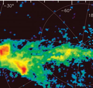
2                                                                                                                                                        Dickey et al.

               telescope. The survey will study the distribution of H i emission and absorption with unprecedented angular and velocity
               resolution, as well as molecular line thermal emission, absorption, and maser lines. The area to be covered includes
               the Galactic plane (|b| < 10°) at all declinations south of δ = +40◦ , spanning longitudes 167◦ through 360◦ to 79◦ at
               b = 0◦ , plus the entire area of the Magellanic Stream and Clouds, a total of 13 020 deg2 . The brightness temperature
               sensitivity will be very good, typically σT  1 K at resolution 30 arcsec and 1 km s−1 . The survey has a wide spectrum of
               scientific goals, from studies of galaxy evolution to star formation, with particular contributions to understanding stellar
               wind kinematics, the thermal phases of the interstellar medium, the interaction between gas in the disk and halo, and the
               dynamical and thermal states of gas at various positions along the Magellanic Stream.
               Keywords: Galaxy: evolution, Galaxy: general, ISM: clouds, ISM: general, ISM: molecules, ISM: kinematics and
               dynamics

               1 INTRODUCTION                                                                          diameter primary reflector. The radiation simply falls on the
               This paper describes a survey of the Milky Way (MW) Galac-                              receiver array, which is carefully impedance matched to min-
               tic plane, the Magellanic Clouds (MCs), and the Magellanic                              imise reflections and other losses, and contains 188 separate
               Stream (MS) that will be carried out at λ 21 cm and 18 cm                               amplifier elements. The signals are then further processed
               to study the atomic hydrogen (H i) and OH lines. The survey                             and combined to make up to 36 independent beams with a
               will reach an unprecedented combination of sensitivity and                              total area on the sky of 30 deg2 . Each of these beams acts like
               resolution, using the revolutionary phased-array feed (PAF;                             the single-dish primary beam of the interferometer, which is
               Chippendale et al. 2010) technology of the Australian Square                            made up of 36 dishes and hence 630 baselines. The wide field
               Kilometre Array Pathfinder (ASKAP) telescope. This tele-                                of view of the small dish-plus-PAF combination leads to a
               scope is currently under construction in Western Australia by                           very high survey speed. With only the effective collecting
               the Australia Telescope National Facility, part of the Com-                             area of a 72-m diameter dish, ASKAP can observe a large
               monwealth Scientific and Industrial Research Organisation,                              area on the sky to a given flux density limit faster than much
               Astronomy and Space Science (CASS) branch. The survey                                   larger radio telescopes that do not have PAFs.
               described here is among a group selected in 2009 to run                                      To detect an unresolved source, the critical telescope pa-
               during the first 5 years of operation of the telescope. In the                          rameter is flux density sensitivity, σF , which is set merely by
               longer term, the design and technology used in ASKAP may                                the total effective collecting area, system temperature, band-
               become the model for the ambitious Square Kilometre Array                               width, and integration time (Johnston & Gray 2006). How-
               (SKA) instrument. In the SKA era, surveys like the one de-                              ever, for a survey of extended emission that is distributed on
               scribed here will advance our knowledge of the Galaxy and                               angular sizes larger than the synthesised beam, it is bright-
               its contents in ways that will revolutionise astrophysics. The                          ness temperature sensitivity, σT , that matters. For a given
               project described in this paper is a step toward that goal.                             total collecting area, the placement of the antennas of the ar-
                  The Galactic ASKAP Survey (GASKAP) is the only ap-                                   ray determines the distribution of baseline lengths and hence
               proved ASKAP project that will have sufficiently high ve-                               both the maximum resolution and the brightness sensitivity.
               locity resolution to study the profiles of the H i and OH lines                         The more widespread the antenna distribution the lower is
               in emission and absorption. It is qualitatively different from                          the filling factor, i.e. the covering factor in the aperture plane,
               the other planned ASKAP surveys in that high brightness                                  f . Lower filling factor results in worse brightness sensitivity,
               temperature sensitivity is the goal for much of the science,                            i.e. higher noise in brightness temperature, σT .
               e.g. for detecting low column densities of gas. This section                                 The ASKAP telescope is a general-purpose instrument,
               describes the strengths of the ASKAP telescope for achiev-                              with baselines up to 6 km in length, but most of the base-
               ing this goal, and the reasons behind the choice of observing                           lines fall in two main groups: one with lengths between 400
               parameters selected for GASKAP. Section 3 discusses some                                and 1200 m and the other between 2 and 3 km (Figure 1).
               of the scientific applications of the survey data, and the ques-                        The ASKAP array was designed to provide optimum perfor-
               tions it will answer. Sections 4–6 describe the planning for                            mance for extragalactic surveys of continuum and spectral
               the survey currently underway through simulations, specifi-                             line sources, hence the two peaks in the baseline distribution.
               cations of the data products, and follow-up observations.                               Fortuitously, these two peaks are very well matched to the
                                                                                                       needs of a Galactic H i survey as well, with the dominant
                                                                                                       shorter baseline peak giving excellent brightness sensitivity
                                                                                                       at beam sizes of 30–60 arcsec, while the longer baselines pro-
               1.1 The ASKAP Telescope                                                                 vide higher resolution (10 arcsec) that will allow us to obtain
               The ASKAP telescope (Johnston et al. 2007, 2008) is inno-                               sensitive H i absorption spectra toward continuum sources
               vative in many ways, the most revolutionary being its focal                             with flux densities as low as 20 mJy. Similarly, emission
               plane on which is mounted a PAF and receiver array. As                                  from the 18-cm lines of OH occurs both in very compact
               currently designed and tested, the PAF uses no feed horns                               maser spots and in very widespread but faint thermal emis-
               or other concentrators of the radiation focused by the 12-m                             sion, while it appears in absorption toward compact, high
               PASA, 30, e003 (2013)
               doi:10.1017/pasa.2012.003

Downloaded from https://www.cambridge.org/core. IP address: 46.4.80.155, on 03 Aug 2021 at 13:11:22, subject to the Cambridge Core terms of use, available at https://www.cambridge.org/core/terms.
https://doi.org/10.1017/pasa.2012.003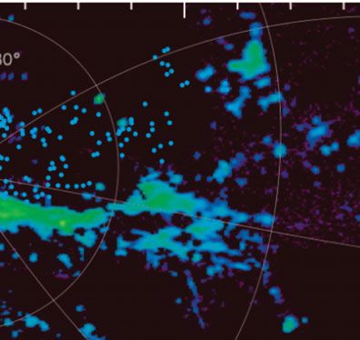
GASKAP—The Galactic ASKAP Survey                                                                                                                                        3

                                                                                                   F

                                          N

                                                                                      B

                                           Figure 1. The ASKAP baseline distribution for a source at δ = −50◦ , from Gupta et al. (2008).
                                           The two peaks at 2–6 kλ (0.4–1.2 km) and 10–15 kλ (2–3 km) are designed to optimise the array
                                           for both extragalactic spectral line and continuum surveys. For a Galactic survey, they are perfectly
                                           placed to measure H i emission and absorption as well as a combination of diffuse OH emission and
                                           OH maser emission. The y-axis gives the number of 1-min samples for a source at δ = −50◦ in a
                                           10-h observation at 1.42 GHz.

            brightness background continuum sources. The ASKAP tele-                                beamwidth. One of the options for ASKAP resolution has
            scope design is an excellent match to the needs of a Galactic                           synthesised beamwidth, θs = 9.7 × 10⁻⁵ rad = 20 arcsec
            survey of emission and absorption in both the H i and OH                                (FWHM), giving  = 1.1 × 10⁻⁸ sr, and for the λ21-cm line
            lines.                                                                                   f /s = 5.8 × 10⁻⁴ . Using B = 1 km s−1  5 × 10³ Hz for
               Following Equations (3) and (4) of Johnston et al. (2007),                           the (heavily smoothed) effective bandwidth and c = s = 1,
            the ASKAP survey speed, S(σT ) in deg2 h−1 is a function of                             the ASKAP survey speed is
            the rms noise in the brightness temperature, σT , as                                                                          2
                                                                                                                                    σT                −1
                                                                       2                                  S(σT ) = 0.10                        deg2 s     (ASKAP),              (3)
                                                             c σT f                                                                Trec
                                S(σT ) = FoV Bnp                             ,            (1)
                                                              Trec s
                                                                                                    and to get sensitivity σT = 2.0 K, this gives S = 0.6 deg2
                                                                                                    h−1 corresponding to integration time per pointing of tint =
            where the field of view (FoV) is 30 deg2 , the bandwidth B                              FoV/S = 50 h.
            is in Hz, the number of polarisations np = 2, the correlator                               For comparison, the Karl G. Jansky Very Large Array
            efficiency c ≤ 1, the expected system temperature of the                               (VLA) C configuration also gives resolution of about θs =
            receivers Trec = 50 K, the synthesis efficiency given by the                            20 arcsec, but N = 27, Trec  37 K (Momjian & Perley 2011,
            taper or weighting of the baselines in the mapping process                              with A  0.6), A = 490 m2 , and FoV = 0.32 deg2 , resulting
            s ≤ 1, and the effective aperture filling factor of the antennas                       in a filling factor f /s = 1.9 × 10⁻³ and a VLA C Array
            is f , where                                                                            survey speed of
                                                  AA Ns                                                                                 2
                                            f =                                           (2)                                        σT
                                                     λ2                                                S(σT ) = 1.1 × 10⁻²                       deg2 s−1   (VLA C array).        (4)
                                                                                                                                     Trec

            with λ being the wavelength in meter, A = 113 m2 be-                                    To get brightness temperature sensitivity σT = 2 K requires
            ing the collecting area of a single antenna, A  0.6 be-                               S = 0.12 deg2 h−1 , which is about one-fifth the speed of
            ing the corresponding aperture efficiency, N = 36 being the                             ASKAP.
            number of antennas, and  = 1.13 θs2 being the solid an-                                   On the other hand, the Arecibo 305-m telescope with
            gle of the synthesised beam in steradians (sr), where θs                                the N = 7 multibeam Arecibo L-band Focal-plane Array
            is the full width at half-maximum (FWHM) synthesised                                    (ALFA) receiver has Trec = 30 K, np = 2, FoV = 3.8 × 10⁻³
            PASA, 30, e003 (2013)
            doi:10.1017/pasa.2012.003

Downloaded from https://www.cambridge.org/core. IP address: 46.4.80.155, on 03 Aug 2021 at 13:11:22, subject to the Cambridge Core terms of use, available at https://www.cambridge.org/core/terms.
https://doi.org/10.1017/pasa.2012.003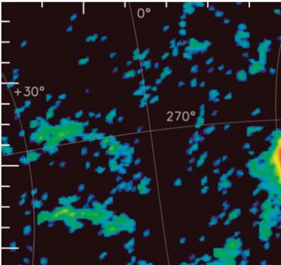
4                                                                                                                                                        Dickey et al.

               deg2 for each beam (Goldsmith 2007), and                                                foreground emission to be subtracted accurately. The optical
                                                       2                                             depth noise is then given by the strength of the continuum
                                             c σT
                     S(σT ) = FoV Bnp N                (Arecibo ALFA)                        (5)       and by σF , not by σT . Thus, the ASKAP telescope provides
                                              Trec
                                                                                                       a great combination of high brightness temperature sensitiv-

                                                σ 2                                                   ity plus high angular resolution that matches the needs of
                                        = 270 c T       deg2 s−1 ,                           (6)
                                                Trec                                                   several different scientific applications. The scientific objec-
                                                                                                       tives of the GASKAP survey are discussed in more detail in
               or S = 170 deg2 h−1 for σT = 0.4 K and c = 1. Note that                                Section 3.
               the filling factor f = 1 for a single-dish telescope with a                                To optimise a survey for mapping low surface brightness
               filled aperture. This survey speed is much faster than any                              emission entails matching the telescope baseline distribu-
               aperture synthesis telescope, but Arecibo’s beam size of θs =                           tion to the scale of the structures of interest. For a perfectly
               3.5 arcmin (at λ21 cm) is far from the 10 arcsec that ASKAP                             smooth brightness distribution, a single-dish antenna is the
               can achieve.                                                                            only tool to use, since interferometers have negative side-
                                                                                                       lobes that partially or completely cancel out the main beam
                                                                                                       response, depending on the image restoration technique, e.g.
               1.2 Survey Description
                                                                                                       clean or maximum entropy methods (Section 4). GASKAP
               The GASKAP survey is one of 10 approved survey science                                  will depend on supplementary observations with single-dish
               projects for ASKAP; its purpose is to study the distribution                            telescopes to fill in the emission with very large angle struc-
               of H i and OH in the MW disk and the Magellanic Sys-                                    ture, corresponding to very short baselines (‘short spacing
               tem. A summary of the survey areas is presented in Table                                flux’), and ultimately any smooth background (‘zero spac-
               1. The GASKAP survey does not seek to cover the entire                                  ing’, meaning a brightness constant over the whole sky). The
               sky, as single-dish surveys such as Galactic All Sky Sur-                               flux sensitivity of an interferometer telescope is calculated
               vey (GASS) (McClure-Griffiths et al. 2009), Leiden Argen-                               by assuming that the source is unresolved, so that even the
               tine Bonn (LAB) (Kalberla et al. 2005, 2010), and Galactic                              longest baselines do not suffer any cancellation due to their
               ALFA (GALFA-HI; Peek et al. 2011a) have done. The in-                                   finely spaced positive and negative sidelobes. The brightness
               terferometer sacrifices brightness sensitivity for resolution,                          sensitivity can only be calculated given an angular size, us-
               so the GASKAP niche is to study regions where the emis-                                 ing the baseline distribution of the antennas, as in Figure
               sion is bright, but with important structure on small angular                           1. Setting the specifications and strategy of a survey such as
               scales and narrow velocity widths. H i emission from the                                GASKAP involves a process similar to impedance matching,
               Galactic plane and the MCs has brightness temperatures of                               where the characteristics of the telescope are optimised for
               tens to more than a hundred K, so σT of 2 K or less is suffi-                           a particular range of spatial frequencies, or angular scales
               cient to provide good signal-to-noise ratio (S/N). OH masers                            of the distribution of the emission on the sky. For ASKAP,
               will appear as bright, unresolved spots of emission; for these                          there are relatively few baselines shorter than 100 m, so a
               the long baselines are needed to maximise the relative po-                              single-dish telescope of this diameter or larger is optimum
               sitional accuracy at different radial velocities in the same                            to fill in the short spacings. The Effelsburg Bonn HI Survey
               source, thus allowing the precise determination of spatial-                             (EBHIS) (Kerp et al. 2011) and GASS (Kalberla et al. 2010)
               velocity structure. High flux density sensitivity is necessary                          surveys will be useful for this purpose.
               for good astrometry so that OH maser positions can be com-                                 Any particular interstellar structure, e.g. a shell, cloud, or
               pared with those of protostellar cores in star formation re-                            chimney of whatever shape and size, has a corresponding flux
               gions, and with asymptotic giant branch (AGB)/post-AGB                                  distribution on the u,v plane, given by the Fourier transform
               stars from optical and infrared (IR) surveys. For H i absorp-                           of its brightness as a function of position on the sky. The
               tion toward background continuum sources, a resolution of                               baselines of the telescope should sample this emission on
               10 arcsec given by the longer ASKAP baselines will allow the                            the u,v plane as completely as possible, to give an image

                                      Table 1. Survey Areas

                                                                                                                              Area         Time          Speed
                                            Component Name                      Location on Sky (see Figure 2)               (deg2 )        (h)        (deg2 h−1 )

                                      Low latitude                           |b| < 2.5◦ , all  for δ < +40◦                  1650         2750           0.60
                                      Intermediate latitude                  2.5◦ < |b| < 10◦ , all  for δ < +40◦            4890         2038           2.40
                                      Magellanic Clouds                      LMC (2) + SMC (1) = 3 deep fields                  90          600           0.15
                                      Magellanic Bridge + Stream             −135◦ < ms a < +66◦ , varying bms a             6390         2662           2.40
                                      Total                                                                                  13020         8050

                                      a Magellanic   Stream coordinates (Nidever et al. 2008); see Figure 3.

               PASA, 30, e003 (2013)
               doi:10.1017/pasa.2012.003

Downloaded from https://www.cambridge.org/core. IP address: 46.4.80.155, on 03 Aug 2021 at 13:11:22, subject to the Cambridge Core terms of use, available at https://www.cambridge.org/core/terms.
https://doi.org/10.1017/pasa.2012.003
GASKAP—The Galactic ASKAP Survey 5
of the best possible fidelity, i.e. dynamic range. For a sur- neous coverage of the 21-cm line of H i at 1420 MHz and
vey, the aggregate distribution of brightness over all angular three of the 18-cm OH lines at 1612, 1665, and 1667 MHz,
scales throughout the survey region should be matched by but not the fourth at 1720 MHz. For studies of H i and OH in
the baseline distribution and integration time of the tele- the MW, MCs, and MS, high velocity resolution is critical.
scope. For the 21-cm line, the u,v distribution of the bright- The ASKAP spectrometer provides a total of 16384 chan-
ness in the aggregate follows a power-law function both in nels on each baseline. These will be allocated to a few narrow
the Galactic plane at low latitudes (Crovisier & Dickey 1983; ‘zoom’ bands with fine velocity resolution. For Galactic ob-
Green 1993; Dickey et al. 2001), in the MCs (Stanimirović & servations, a good choice of channel spacing is 976.6 Hz,
Lazarian 2001), and in the Magellanic Bridge (MB; Muller giving a velocity step of 0.18–0.21 km s−1 (see Table 2).
et al. 2004). The power law is steep, having index −2.5 to These narrow spectrometer channels will cover the four lines
−3.5 typically; therefore, given the ASKAP baseline distri- with LSR velocity ranges of ±760 km s−1 for H i (7394
bution on Figure 1, a reasonable goal for the survey is to channels) and ±311 km s−1 for the OH lines (3419 channels
obtain σT somewhat below 2 K on angular scales of 20 arc- at 1612 MHz and 5571 channels covering both the 1665-
sec. On smaller scales, the emission is very faint and the u,v and 1667-MHz lines together). Since the OH main lines are
coverage of the telescope is relatively sparse for baselines separated by just 352 km s−1 , blending of the two lines is
longer than about 2 km, so very long integration time would possible in directions where the radial velocity of the emis-
be needed to push beyond this sensitivity goal. The longer sion spreads over more than this amount. This is not expected
baselines are useful for absorption spectra toward compact in the GASKAP survey area. The allowed velocity range due
continuum background sources, where brightness sensitivity to Galactic rotation in the inner Galaxy, excepting the Galac-
is not the limiting factor. tic Center, covers about −150 to +150 km s−1 maximum,
Besides the MW and MCs, GASKAP will discover and depending on longitude. In the MCs and MS, the velocity
map the dynamics of dwarf galaxies in the local volume out ranges from about +450 km s−1 in the leading arm (Kilborn
to Local Standard of Rest (LSR) velocities of ±700 km s−1 . et al. 2000) to −400 km s−1 (LSR) near the northern tip of
Faint, irregular dwarfs typically have narrow Gaussian H i the MS.
profiles due to their low rotational velocities. Their linewidths
are similar to those of high-velocity clouds (HVCs), but their
1.3 Survey Parameters
velocity fields are generally very different. Searching for gas-
rich, local-group dwarf galaxies is particularly important in GASKAP will use three different survey speeds, with inte-
the GASKAP survey area at low Galactic latitudes. This gration times of 12.5, 50, and 200 h, which correspond to S =
science goal overlaps that of the WALLABY project (B. 2.4, 0.6, and 0.15 deg2 h−1 . These translate to brightness tem-
Koribalski et al., in preparation) that will cover the whole perature sensitivities at different angular resolutions as given
sky with a velocity resolution of ∼4 km s−1 and 300-MHz in Table 3; smoothing to larger beam area gives much lower
bandwidth. values of the noise in brightness temperature, σT . The flux
As a pathfinder to the SKA, the frequency range of ASKAP density sensitivity, given in the last column of Table 3, is only
was chosen to be 700 MHz to 1.8 GHz, with a maximum a weak function of angular resolution. The lowest flux density
instantaneous bandwidth of 300 MHz. This allows simulta- noise level, σF , is achieved with resolution 20 arcsec; at this
Table 2. Frequency and Velocity Coverage.
Frequency LSR Velocity Channel
Range Range Spacing
Band (MHz) (km s−1 ) (km s−1 )
Hi 1416.795–1424.016 ±762 0.206
OH 1612 1610.561–1613.900 ±310 0.182
OH main lines 1663.657–1669.099 ±313 0.176
Table 3. Survey Speeds and Sensitivity.
σT (K), B = 5 kHz
Map Dwell for θFWHM (arcsec) =
Speed Time σF (mJy)
Survey Component (deg2 h−1 ) (h) 20 30 60 90 180 B = 5 kHz
Magellanic Clouds 0.15 200 1.01 0.48 0.21 0.12 0.05 0.5
Low latitude 0.60 50.0 2.02 0.96 0.42 0.24 0.10 1.0
Intermediate latitude + MS 2.40 12.5 4.05 1.91 0.85 0.49 0.20 2.0
PASA, 30, e003 (2013)
doi:10.1017/pasa.2012.003
Downloaded from https://www.cambridge.org/core. IP address: 46.4.80.155, on 03 Aug 2021 at 13:11:22, subject to the Cambridge Core terms of use, available at https://www.cambridge.org/core/terms.
https://doi.org/10.1017/pasa.2012.0036 Dickey et al.
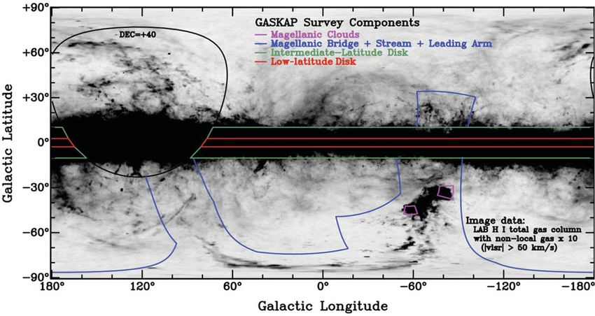
Figure 2. The GASKAP survey areas in Galactic coordinates, with H i column densities from the LAB
survey in the background. The region north of δ = +40◦ must be filled in from the Northern Hemisphere.
The Galactic and Magellanic Emission Survey (GAMES) described in Section 6 will cover the region
north of δ = +40◦ .
resolution all baselines have roughly equal weights (s = 1). 2 COMPARISON WITH OTHER SURVEYS
Just three ASKAP fields are enough to cover most of the area
The brightness temperature sensitivity versus angular resolu-
of the MCs, which will have a 200-h integration time per
tion for the low-latitude GASKAP survey component, which
pointing or ‘Dwell Time’ (Table 3, column 3). A single line
will be observed using the intermediate mapping speed of
of 55 fields centered at b = 0◦ each with a 50-h integration
0.60 deg2 h−1 (middle row of Table 3), is illustrated in
time results in a very sensitive survey of the Galactic plane
Figure 4, along with the corresponding sensitivities of three
(|b| < 2.5◦ ) over longitudes 167◦ through 360◦ (the Galactic
recent aperture synthesis surveys of the Galactic plane, the
Center) to 79◦ . An intermediate latitude strip of four rows
Southern Galactic Plane Survey (SGPS; McClure-Griffiths
of fields covers |b| ≤ 10◦ , centered at b = ±2.5◦ and ±7.5◦ .
et al. 2005), the Canadian Galactic Plane Survey (CGPS; Tay-
These are observed at the fastest survey speed, with an inte-
lor et al. 2003), and the VLA Galactic Plane Survey (VGPS;
gration time of 12.5 h on each pointing. Finally, a wide area
Stil et al. 2006). Also shown in Figure 4 are the sensitivities
(about 6400 deg2 ) of the MS is covered at the fastest survey
and resolutions of the GALFA-HI (Stanimirović et al. 2008;
speed (12.5 h per pointing). These areas are illustrated in
Peek et al. 2011a) seven-beam single-dish survey and the
Figures 2 and 3.
lower resolution, all-sky, EBHIS survey. The GASS survey
BMS
LMS
Figure 3. The GASKAP MS survey area with axes labeled in MS coordinates and H i column densities from the LAB survey in the background (Nidever
et al. 2010). The white squares represent ASKAP pointings with the shorter integration time (12.5 h), while the red squares are pointings that will be observed
for either 50 or 200 h.
PASA, 30, e003 (2013)
doi:10.1017/pasa.2012.003
Downloaded from https://www.cambridge.org/core. IP address: 46.4.80.155, on 03 Aug 2021 at 13:11:22, subject to the Cambridge Core terms of use, available at https://www.cambridge.org/core/terms.
https://doi.org/10.1017/pasa.2012.003GASKAP—The Galactic ASKAP Survey 7
T
Figure 4. The GASKAP brightness temperature sensitivity (σT ) vs. resolution (θs ) with spectra smoothed to 1
km s−1 . The solid curve represents the medium integration time of 50 h per pointing, while the other two survey
speeds have integration times four times longer or shorter, and hence they have sensitivities a factor of 2 higher
or lower, indicated by the dashed lines (see Table 3). On the left (θs 20 arcsec) are combinations appropriate
for OH maser emission and H i absorption at low latitudes, and on the right (θs 1 arcmin) are combinations
appropriate for low column density H i in the MS and diffuse OH emission in the Galactic plane. H i emission
mapping at low latitudes will make use of resolution from 20 arcsec to 1 arcmin, depending on the brightness and
angular scales of the emission in each field. The GALFA-HI point is based on a 10-s integration per beam area,
smoothed to resolution θ = 4 arcmin.
would be off-scale in the lower right. For GASKAP, the Spitzer Space Telescope at 24–160 μm) and submillime-
lower angular resolution cubes (1.5–3 arcmin) are obtained ter (5–36 arcsec for the Herschel Space Observatory at 70–
from the same data as the high-resolution images by smooth- 500 μm). GASKAP data cubes will thus provide a well-
ing in the image plane or by tapering more heavily in the u, v matched comparison of H i with interstellar medium (ISM)
(aperture) plane. This taper reduces the effective collecting tracers at IR, millimeter, and submm wavelengths. With this
area of the array (s < 1) for larger beamwidths, so that the survey, it will finally be possible to obtain images of struc-
slope of the line in Figure 4 is not as steep as −2, as expected tures in the atomic (H i) medium with the richness and detail
from Equations (1) and (2) [ f ∝ σT−1 with all other quantities routinely available for the dust and molecular gas.
fixed in Equation (1), and f ∝ ∝ θs2 in Equation (2), but
s decreases weakly with increasing θs ]. The GASKAP sur-
vey is composed of different surveys done simultaneously; 3 SCIENTIFIC GOALS OF THE SURVEY
the output data from each one will be useful for a variety of This section presents a series of short scientific discussions
applications that require different combinations of sensitiv- that motivate the different applications of the GASKAP sur-
ity and resolution, as indicated in Figure 4 and discussed in vey. Because of the versatile capabilities of the telescope and
Section 3. spectrometer, all of these goals are achieved simultaneously
The trade-off between resolution and brightness tempera- with the same observations. For study of the interstellar H i
ture sensitivity apparent in Table 3 is at once the limitation and OH of the MW and Magellanic System, the fine veloc-
and the great power of an aperture synthesis survey of dif- ity resolution of GASKAP is critical, and even more so for
fuse emission. For Galactic and Magellanic H i emission, OH masers. As high spectral resolution is what distinguishes
the 30 arcsec and 0.2 km s−1 resolutions of GASKAP are a GASKAP from the other ASKAP survey projects, the sci-
breakthrough, because they provide spectral line cubes com- ence goals mostly are formulated to take advantage of the
parable with the best images from surveys like those from narrow spectral channels and high brightness sensitivity that
space-based telescopes in the far-IR (6–40 arcsec from the will be obtained.
PASA, 30, e003 (2013)
doi:10.1017/pasa.2012.003
Downloaded from https://www.cambridge.org/core. IP address: 46.4.80.155, on 03 Aug 2021 at 13:11:22, subject to the Cambridge Core terms of use, available at https://www.cambridge.org/core/terms.
https://doi.org/10.1017/pasa.2012.0038 Dickey et al.
3.1 Galaxy Evolution Begins at Home ing structures such as chimneys and shells. We will study
this motion primarily in H i cubes that show the velocity
One of the great challenges of modern astrophysics is under-
structure of the diffuse medium, supplemented by more de-
standing how galaxies form and evolve. This is intimately
tailed maps of molecular clouds in diffuse OH emission and
connected with the outstanding problem of star formation: as
OH masers in regions of massive star formation. These are
star formation transforms the ISM, adding heavy elements
the sources of the feedback that stirs up the gas (Ford et al.
and kinetic energy, it determines the structure and evolution
2008; Ford, Lockman, & McClure-Griffiths 2010; Dawson
of galaxies. While modern cosmological theories can predict
et al. 2011b). Clouds of neutral, atomic gas in the MW halo
the distribution of dark matter in the Universe quite well,
are excellent targets for the GASKAP survey because of its
predicting the distribution of stars and gas in galaxies is still
high angular resolution. Several examples have been studied
extremely difficult (Tasker et al. 2008; Putman et al. 2009;
with a resolution of 30 arcsec with the VLA (Pidopryhora,
Tonnesen & Bryan 2009). The reason for this is the com-
Lockman, & Rupen 2009); on this scale, they show sharp
plex and dynamic ISM: simulations reach a bottleneck on
density contrasts that suggest that they are unstable in var-
scale sizes where a detailed understanding of star formation,
ious ways, particularly to Rayleigh–Taylor fragmentation.
its feedback, and the interaction between galactic disks and
Thus, cloud mapping in H i can reveal the evolution and dy-
halos needs to be included (Stanimirović 2010). To make
namics of the gaseous halo. GASKAP is designed to trace the
advances in the area of galaxy formation and evolution, we
effects of this feedback throughout the MW disk and lower
must begin with our home neighborhood where the physics
halo.
that drives this process can be exposed and studied in detail.
The GASKAP survey focuses on the generic physical pro-
cesses that drive galaxy evolution by revealing their astro- 3.3 How Galaxies Get Their Gas
physical basis here at a redshift of z = 0. GASKAP will
How much gas flows in and out of the disk through the halo,
provide a new and vastly improved picture of the distribution
how fast does it flow, and what forces act on it along the way?
and dynamics of gas throughout the disk and halo of both
How do halo clouds survive their trip down to the disk? These
the MW and the MCs. The data will provide the image detail
questions can be studied through H i structure in the MS
and broad range of scale sizes that are essential for a quan-
and HVCs (Putman, Saul, & Mets 2011), which reveals the
titative understanding of the physics of the gas in the MW
conditions of the outer halo, and in the disk–halo interface,
and MCs, including the effects of radiation, shocks, mag-
where the Galactic fountain constantly circulates H i as evi-
netic fields, and the shapes of the gravitational potentials of
denced by chimneys and H i clouds (Stanimirović et al. 2006;
the disk and halo. Comparing the mixture of warm, cool, and
Lockman 2002; Ford, Lockman, & McClure-Griffiths 2010;
molecular ISM phases in the MW and the MCs shows the
Marasco, Fraternali, & Binney 2012). In low-mass galaxies,
variation of the heating and cooling rates with metallicity,
outflows are a determining factor in setting the rate of their
and how these processes affect the star formation rate. The
gradual chemical enrichment. The 30 Doradus mini-starburst
MCs studied with GASKAP resolution in position and ve-
in the Large Magellanic Cloud (LMC) may be responsible
locity will show two entire galactic systems in enough detail
for part of the MS, either as source or sink (Nidever et al.
to trace the connection between star formation and gas infall
2008; Olsen et al. 2011), and the actively star-forming SMC
and outflow. The specific astrophysical processes accessible
has a porous ISM from which gas easily escapes, yet it is
to the survey are the initial conditions for star formation and
still extremely gas rich (Figure 5). As outflow and accretion
ISM phase transitions, the feedback processes in the ISM,
rates are expected to be a dramatic function of galaxy mass,
and the exchange of matter between the disk and the halo.
GASKAP’s comparison of the disk–halo mass exchange in
the MW and the MCs will probe the variability of crucial
physical parameters governing the large-scale gas flows in
3.2 Feedback Processes—Wild Cards in Galaxy
three galaxies of very different masses in the range where
Evolution
these rates are expected to change dramatically.
Galaxy evolution is largely driven by star formation and the Cosmological simulations predict that gas accretion onto
subsequent enrichment of the interstellar gas with heavy ele- galaxies is ongoing in the present epoch. The fresh gas is
ments through red giant winds and supernova explosions. By expected to provide fuel for star formation in galaxy disks
undertaking an unbiased, flux-limited survey of OH masers (Maller & Bullock 2004). Some of the H i we see in the halo
in the MW and the MCs, GASKAP will image the gas at of the MW comes from satellite galaxies, some is former
both ends of this cycle: the first stages of high-mass star disk material that is raining back down as a galactic fountain,
formation and the last evolutionary phases of both the mas- and some may be condensing from the hot halo gas (Putman
sive (8–25 M ) supergiant progenitors of Type II supernovae et al. 2009; Brooks et al. 2009).
and the more plentiful low- and intermediate-mass stars, i.e. Just how gas gets into galaxies remains a mystery. The
oxygen-rich AGB stars to planetary nebulae (PNe). large number of gas clouds clearly visible in the Galactic
The motion of the gas in the disk and halo traces both halo is one potential source. HVCs fall into several distinct
stochastic processes such as turbulence and discrete, evolv- populations (Wakker & van Woerden 1991), some associated
PASA, 30, e003 (2013)
doi:10.1017/pasa.2012.003
Downloaded from https://www.cambridge.org/core. IP address: 46.4.80.155, on 03 Aug 2021 at 13:11:22, subject to the Cambridge Core terms of use, available at https://www.cambridge.org/core/terms.
https://doi.org/10.1017/pasa.2012.003GASKAP—The Galactic ASKAP Survey 9
Figure 5. Locations of background continuum sources toward the SMC. The circles show
directions for which the H i absorption spectra have already been measured. The crosses show
locations of sources bright enough to give good quality absorption spectra with GASKAP.
with the MS and other clouds possibly decelerated by the hot 3.4 Disk–Halo Mass Exchange and the Energy Flow
halo (Olano 2008). One exemplar HVC system, known as in the ISM
the Smith Cloud (Lockman et al. 2008), is interesting as a
rare example of a fast-moving massive stream (∼107 M ) For H i emission, the GASKAP survey will provide the
close to the plane of the disk. The Smith Cloud has roughly biggest improvement over existing survey data in the range
equal amounts of neutral and ionised hydrogen gas (Bland- 20−90 arcsec with a tenfold increase in resolution in most
Hawthorn et al. 1998; Hill et al. 2009) and appears to have areas. The Galactic plane has been mostly covered at low
punched through the disk in the last 100 Myr (Lockman latitudes (|b| < 1◦ or greater in some regions) by the combi-
et al. 2008). It is difficult to understand how this cloud has nation of the Canadian, Southern, and VLA Galactic Plane
survived hitting the disk, or even its passage through the hot Surveys (Taylor et al. 2003; McClure-Griffiths et al. 2005;
halo (e.g. Heitsch & Putman 2009). And yet, if we are to Stil et al. 2006) with resolution ranging from 1–2 arcmin
form a complete picture of the life cycle of the Galaxy, it and brightness sensitivity 1.5–3 K rms, and GALFA-HI at
is imperative that we understand how systems like Smith’s 4 arcmin resolution and sensitivity 0.1–1 K rms (Peek et al.
Cloud and the Magellanic System interact with the Galactic 2007). From these surveys we get a hint of the glorious im-
disk. ages that GASKAP will produce. The hierarchy of structure
GASKAP will provide complete, high-resolution cover- and motions of the ISM begins on scales of kiloparsecs,
age of the MS and HVCs associated with its Leading Arm where we see how spiral arms influence gas streaming mo-
(LA) as well as all HVCs that come within 10◦ of the tions, shocks, and star formation (McClure-Griffiths et al.
Galactic plane. A different ASKAP survey, WALLABY (B. 2004; Strasser et al. 2007). Continuing to 10−100 pc scales,
Koribalski et al., in preparation), will complement GASKAP we see shells, bubbles, and chimneys that trace the collective
by providing low spectral resolution images of Galactic, as effects of many supernova remnants and stellar winds (Nor-
well as extragalactic, H i over the entire sky. The all-sky mandeau, Taylor, & Dewdney 1996; Stil et al. 2004; Kerton
coverage of WALLABY’s Galactic H i component will be et al. 2006; McClure-Griffiths et al. 2006; Kang & Koo 2007;
useful for tracing full gas streams, such as Smith’s Cloud, Cichowolski et al. 2008). Moving down to scales of 1 pc and
over large areas of the sky. By working with WALLABY smaller reveals tiny drips and cloudlets in shell wall insta-
to provide the context, GASKAP will be able to study the bilities (McClure-Griffiths et al. 2003; Dawson et al. 2011a,
processes at work as HVC streams approach the Galac- 2011b), small-scale structure formed in colliding flows in
tic disk. The spectral resolution of GASKAP will allow the turbulent disk ISM (Vázquez-Semadeni et al. 2006; Hen-
measurement of the cooling, fragmentation, and decelera- nebelle & Audit 2007) and ram-pressure interactions between
tion of H i halo clouds as they near the plane and com- HVCs and the hot Galactic halo gas (Peek et al. 2011a).
parison with models such as those of Heitsch & Putman Some recent H i detections in dust shells around
(2009). AGB and post-AGB stars mapped by the Infrared Space
PASA, 30, e003 (2013)
doi:10.1017/pasa.2012.003
Downloaded from https://www.cambridge.org/core. IP address: 46.4.80.155, on 03 Aug 2021 at 13:11:22, subject to the Cambridge Core terms of use, available at https://www.cambridge.org/core/terms.
https://doi.org/10.1017/pasa.2012.00310 Dickey et al.
Observatory (ISO) (e.g. Libert, Gèrard, & Le Bertre 2007) allows the excitation temperature and column density at each
indicate that GASKAP could provide a larger catalogue of velocity to be measured separately, giving a good estimate of
such shells. Considering that the distribution of PNe in height the kinetic temperature. The ambient pressure is tied to the
above the midplane, Z, follows that of the OH/IR stars (e.g. equilibrium temperature through the cooling function of the
the Macquarie/AAO/Strasbourg Hα catalogue (MASI-I) cat- H i (Field, Goldsmith, & Habing 1969; Dalgarno & McCray
alogue; Miszalski et al. 2008), many PNe will be found at 1972). Separating the emission and absorption spectra
intermediate Z heights (0.3–1.0 kpc above the plane) and so requires good angular resolution to allow the emission to be
separated from most of the disk gas in the spectrum, and measured very near to the continuum source. The highest
hence their shells may be detectable in H i. The interac- resolution of the ASKAP array, 10 arcsec, will be excellent
tion of stellar winds and supernova remnants with the ISM for eliminating confusion due to small-scale variations
drives interstellar turbulence, seen in the ionised, neutral, in the emission. Absorption-line studies with GASKAP
and molecular phases with very similar spatial power spectra will be very valuable for understanding the huge range of
(Lazarian & Pogosyan 2000, 2006; Haverkorn et al. 2006). physical conditions now being found in the neutral ISM
The GASKAP data will allow the power spectra of the ISM (Jenkins & Tripp 2011; Peek et al. 2011b). As an example,
turbulence to be measured in a variety of different environ- Figure 5 shows the level of improvement GASKAP will
ments, with greater precision, and over a broader range of make relative to previous studies of absorption in the
scales than any survey of neutral gas has done before. Small Magellanic Cloud (SMC). Only a handful of H i
absorption measurements exists for both the SMC and
the LMC. White crosses in Figure 5 show the location
3.5 Phase Changes in the Gas on Its Way to Star
of radio continuum sources behind the SMC suitable for
Formation
absorption measurements with GASKAP, while the white
What is the relationship between the atomic and molecu- circles show what has been done previously by Dickey et al.
lar phases of the ISM in different interstellar environments? (2000).
GASKAP will trace these phases through H i emission, H i The H i absorption spectra toward continuum sources that
absorption, and diffuse OH emission. Comparing them over GASKAP produces will yield a rich set of gas tempera-
a large area that contains many kinds of clouds, some form- ture, column density, and velocity measurements over most
ing stars and some not, will show how and where the gas of the Galaxy. Matched with these will be complemen-
makes the transition from one phase to another. How does tary, contiguous maps of the cold H i structure and dis-
the temperature of the gas vary, and how are the different tribution from H i self-absorption (HISA) against Galactic
thermal phases mixed in different interstellar environments? H i background emission (Gibson et al. 2000; Gibson 2010).
GASKAP will investigate this by comparing emission and HISA arises from H2 clouds as well as dense H i clouds
absorption spectra to measure the excitation temperatures of actively forming H2 , so it directly probes molecular conden-
the H i and OH lines. sation prior to star formation (Kavars et al. 2005; Klaassen
In H i absorption, GASKAP will be an even greater et al. 2005). A cloud’s age can be estimated by compar-
advance over existing surveys than it is in H i emission. We ing its HISA and molecular content with theoretical models
expect four extragalactic continuum sources per deg2 with (Goldsmith et al. 2007; Krčo et al. 2008). GASKAP’s low-
a peak flux density, F, of 50 mJy or greater, and 10 sources latitude survey will easily map the HISA from a 10−20 K
per deg2 with F > 20 mJy (Condon & Mitchell 1984; Petrov cloud with NH i > 3 × 1018 cm−2 . This sensitivity, enough
et al. 2007). This is at least a factor of 5 more absorption to see the traces of H i in molecular cloud cores, plus cold
spectra at this noise level than in any previous low-latitude atomic gas in H i envelopes around the cores, will be applied
survey. The rms noise is σF 1 mJy in a spectral channel to most of the Galactic disk, enabling comprehensive popu-
of width δv = 1 km s−1 in the low-latitude survey area. This lation studies of H2 -forming clouds, including their proxim-
gives optical depth noise of στ ≤ 0.02 in the absorption ity to spiral shocks (Minter et al. 2001; Gibson et al. 2005).
spectrum toward a source with F = 50 mJy. These spectra GASKAP HISA will offer a rich new database for rigorous
will have excellent S/N in absorption. The more abundant, tests of theoretical models of gas-phase evolution in spiral
fainter continuum sources will give absorption spectra of arms (Dobbs & Bonnell 2007; Kim et al. 2008) including
lower quality (e.g. στ = 0.05 for F = 20 mJy) that will phase lags between spiral shocks and star formation (e.g.
be useful for statistical studies of the cool gas distribution, Tamburro et al. 2008). On much smaller scales, the turbu-
either by co-adding many spectra or by integrating over lent froth of HISA filaments that appear to be pure cold
velocity intervals much broader than 1 km s−1 . H i will be revealed at threefold finer angular and velocity
The big question that the absorption spectra will help an- resolution in GASKAP than in all prior surveys, with suf-
swer is how the thermal interstellar pressure, which changes ficiently improved sensitivity to follow their spatial power
by several orders of magnitude from the midplane to the spectrum down to subparsec scales. This investigation will
lower halo and from the inner Galaxy to the outer disk, deter- relate clouds’ turbulent support to their stage of molecular
mines the mixture of warm and cool H i (Wolfire et al. 1995, condensation. Both 21-cm continuum absorption and self-
2003). Combining 21-cm absorption and emission spectra absorption toward Galactic objects, including masers, are
PASA, 30, e003 (2013)
doi:10.1017/pasa.2012.003
Downloaded from https://www.cambridge.org/core. IP address: 46.4.80.155, on 03 Aug 2021 at 13:11:22, subject to the Cambridge Core terms of use, available at https://www.cambridge.org/core/terms.
https://doi.org/10.1017/pasa.2012.003GASKAP—The Galactic ASKAP Survey 11
helpful for distance determinations (e.g. Anderson & Bania
2009; Green & McClure-Griffiths 2011).
3.6 Diffuse Molecular Clouds Traced by Extended
Wind speed (km s−1)
OH Emission
In addition to H i spectroscopy, GASKAP will further en-
hance the exploration of gas-phase evolution with a new
view of molecular clouds. The OH λ 18-cm lines have long
been used as an alternative to the standard CO proxy for H2 ,
which is subject to the vagaries of ultraviolet shielding, in-
terstellar chemistry, and sub-thermal excitation at densities
below 103 cm−3 (Liszt & Lucas 1996, 1999; Grenier et al.
2005; Sheffer et al. 2008; Wolfire et al. 2010). However, dif-
fuse OH emission is typically about 100 times fainter than
the H i 21-cm line, and there have been no large-area OH
surveys since the ambitious survey of Turner (1979) with
the Green Bank 43-m telescope. ASKAP’s new capabili-
ties bring an unbiased and detailed view of the OH sky Figure 6. Expected distributions of OH masers in AGB stars and red super-
within reach at last. By simultaneously mapping cold H i giants based on empirical scaling relations in Marshall et al. (2004). Open
symbols are known masers, with circles for the Galactic Center region and
self-absorption at 20–60 arcsec resolution and diffuse OH at
squares for the LMC; filled symbols are predictions for GASKAP detections,
90–180 arcsec resolution (to achieve the necessary brightness with triangles for SMC masers.
sensitivity), GASKAP will directly probe the H2 formation
process by providing a comprehensive H i + OH database
of diffuse molecular clouds. These data can be compared to sity greater than 1 Jy at 1.4 GHz on average every 18 deg2 ,
quiescent evolutionary models (e.g. Goldsmith et al. 2007; but in the Galactic plane there will be many more H ii regions
Liszt 2007) and converging-flow dynamical models (e.g. and supernova remnants with flux densities well above 1 Jy,
Bergin et al. 2004; Vázquez-Semadeni et al. 2007) to ad- up to several per degree of longitude for || < 25◦ . Thus, we
dress a key question in the field: How long do H2 clouds take expect many OH absorption spectra for comparison with H i
to form from the diffuse ISM, and how does this affect star absorption.
formation?
Measurement of cloud total column density, tempera-
3.7 OH Masers in Young and Evolved Stars
ture, mass, and other properties will be needed to interpret
millimeter-wave molecular line surveys, IR dust emission OH masers allow us to study stellar birth and death, and give
surveys, and other future Galactic observations. Of particular a picture of Galactic structure and dynamics complementary
interest would be a broad-based analysis of cold H i, OH, CO, to that shown by the interstellar gas. The OH portion of the
and dust in diffuse clouds throughout the Galaxy to establish GASKAP survey will allow study of the sites of high-mass
a common evolutionary clock for clouds seen with multiple star formation and the old stars such as AGB stars, central
tracers. GASKAP’s 3σ OH 1667-MHz sensitivity translates stars of young PNe, and red supergiants that exhibit copious
to a minimum detectable H2 column of ∼1.0 × 1021 cm−2 for gas ejection in the last stages of their evolution. This phase
a 2 km s−1 wide line at 180-arcsec resolution, which is suf- of stellar evolution is a critical contributor to the chemical
ficient to sample the molecular content of an AV ∼ 0.6 mag enrichment of the ISM. OH maser spectra enable us to study
diffuse molecular cloud, or the early OH formation in a dense the energetics of outflows from massive young stellar objects
molecular cloud. This sensitivity will exceed that reached by (YSOs) and the mass-loss rates of dying stars by combining
Turner (1979) with better velocity sampling and with angu- the measured radial velocities with estimates of the gas den-
lar resolution an order of magnitude sharper over a larger sity in and around the OH emission region. With a sensitivity
and unbiased area, including the hitherto unexplored fourth at least one order of magnitude better than previous spatially
Galactic quadrant. At the same time, OH absorption toward limited surveys of OH masers (e.g. Caswell & Haynes 1987;
continuum sources will be probed along with H i absorption Sevenster et al. 2001), and taking into account the number of
to show the excitation temperatures of the 18-cm mainlines. known OH maser sources to date (∼2300 in evolved stars;
Assuming optical depths of a few times 10−3 (Liszt & Lucas Engels, Bunzel, & Heidmann 2010), we expect to find several
1996) and rms noise of 1 mJy for a velocity resolution of thousand new OH maser sources (Figure 6). Such a sensitive
1 km s−1 (Table 2), then background sources brighter than and unbiased survey will allow us to make statistical stud-
about 1 Jy will show detectable absorption in OH. Counting ies of the processes in these evolutionary phases as well as
only extragalactic radio sources, there is one with flux den- proper comparisons with results of Galactic surveys at other
PASA, 30, e003 (2013)
doi:10.1017/pasa.2012.003
Downloaded from https://www.cambridge.org/core. IP address: 46.4.80.155, on 03 Aug 2021 at 13:11:22, subject to the Cambridge Core terms of use, available at https://www.cambridge.org/core/terms.
https://doi.org/10.1017/pasa.2012.00312 Dickey et al.
wavelengths. The total number of OH maser sources is also theless, the detection of a particular maser transition toward
helpful in estimating the net mass ejection rate from stars in a region indicates the presence of a relatively narrow range
the Galaxy and in understanding the circulation of processed of physical conditions in the vicinity. Ellingsen et al. (2007)
material back into the ISM. suggest that the presence and absence of different maser tran-
The accuracy of the point-source position measurement is sitions toward a region can be used as an evolutionary clock
σθ θ /[2(S/N)], where θ = θs is the FWHM of the syn- for the high-mass star formation process and proposed a time
thesised beam, and S/N is the signal-to-noise ratio of the sequence involving all the common maser transitions. Recent
source (e.g. Reid et al. 1988). For strong maser emission studies of methanol and water masers have further refined and
(>0.5 Jy) with spatial-velocity structure, subarcsecond ve- quantified the maser-based timeline (e.g. Breen et al. 2010a,
locity gradients will be measurable by finding the centroid 2010b; Ellingsen et al. 2011). The sensitive GASKAP study
of the emission in each velocity channel. This will allow the represents a unique opportunity to robustly test and refine the
tracing of kinematic structures such as disks or outflows in way that ground-state OH maser emission fits in the timeline.
some OH maser stars, including highly collimated jets and OH masers are generally thought to arise later than water
‘super winds’ in some objects (Sahai et al. 1999; Cohen et al. and class II methanol masers in the evolution of high-mass
2006). GASKAP will allow us to obtain a complete catalogue star formation regions, but to persist after water and class
of evolved stars in special transition phases, of which there II methanol switch off (Forster & Caswell 1989; Breen et al.
are only a few members known so far. Zijlstra et al. (1989) 2010b). Most OH masers in high-mass star formation regions
catalogue several examples of such evolved stars showing are strongest in the 1665-MHz transition, with weaker 1667-
both radio continuum and OH maser emission, which could MHz emission and no 1612- or 1720-MHz maser emission.
be extremely young PNe. Moreover, the shape of OH maser There are, however, exceptions to this pattern (e.g. Caswell
spectra can help identify stars just leaving the AGB phase, 1999; Argon, Reid, & Menten 2003) and GASKAP repre-
when their spectra depart from the typical double-peaked sents the best opportunity to determine if the currently known
profile. An extreme example are those evolved objects un- exceptions represent unusual objects or perhaps short-lived
dergoing highly collimated jets, such as ‘water fountains’ evolutionary phases. Caswell (1999) found that the majority
(Imai et al. 2007). These special types of objects are key to of high-mass star formation regions with a 1612-MHz OH
understanding the evolution and morphology of PNe. maser were not associated with class II methanol masers,
Using the systemic velocities of masers in OH/IR stars, suggesting that these are generally older, more evolved star
GASKAP will allow study of Galactic kinematics as traced formation regions. Argon et al. (2003) found weak (200-mJy
by this stellar population with much more detail and spatial peak) 1665- and 1667-MHz OH masers toward the edges of
extent than previously (e.g. Baud et al. 1981; Sevenster et al. a bipolar outflow traced by water masers toward the Turner–
1999). This will provide a picture of MW stellar dynamics Welsh object near W3(OH). The Turner–Welsh object is a
that complements those from the gas and from the very dif- protostar with a synchrotron jet which is too young, or not
ferent stellar populations that will be sampled by GAIA at sufficiently massive, to have produced an H ii region. So the
optical wavelengths. Argon et al. discovery appears to show that some OH masers
Interstellar masers are one of the most readily detected are associated with very different objects from the high-mass
signposts of locations where high-mass stars are forming. protostars which traditionally show strong ground-state OH
Surveys for masers are able to detect high-mass star forma- maser emission. However, if the luminosity of the masers
tion regions throughout the Galaxy (e.g. Green et al. 2009), in the Turner–Welsh object is typical, then no previous OH
and the number of detected masers suggests that all high- maser survey would have been sensitive to this class of object
mass star formation regions go through a phase where they over a significant volume of the Galaxy. With a 5σ detec-
have associated masers. There are four different types of tion limit in a 0.2 km s−1 spectral channel of approximately
interstellar masers commonly observed in high-mass star 10 mJy (for the low-latitude survey), it will be possible to
formation regions — ground-state OH masers at 1665 and determine what fraction of the water and class II methanol
1667 MHz, 22 GHz water masers, class II methanol masers masers have associated OH masers with peak flux densities
(most commonly at 6.7 and 12.2 GHz) and class I methanol significantly less than 0.5 Jy and also to detect any weak OH
masers (most commonly at 36 and 44 GHz). In addition to the masers which are not associated with other types of masers.
common maser transitions, which are often (but not always) Simultaneous observations of three of the four ground-state
very strong, some sources also show maser emission from ex- OH maser transitions, combined with a growing amount of
cited state OH transitions and/or higher frequency methanol existing data on class I and II methanol masers and water
transitions. These rarer masers are invariably weaker than the masers, will enable us to substantially refine and improve
common masers observed in the same source (e.g. Ellingsen the maser-based evolutionary clock for high-mass star for-
et al. 2011). Studies of the pumping mechanism of the com- mation regions. The strong Zeeman splitting experienced by
monly observed star formation masers show that the observed ground-state OH transitions means that many OH masers in
transitions are less selective than some of the rarer maser star formation regions are highly (up to 100%) circularly po-
transitions and are inverted over a wider range of physical larised and can be used to measure the total magnetic field
conditions (e.g. Cragg, Sobolev, & Godfrey 2003). Never- in the maser region. The spatial resolution of the GASKAP
PASA, 30, e003 (2013)
doi:10.1017/pasa.2012.003
Downloaded from https://www.cambridge.org/core. IP address: 46.4.80.155, on 03 Aug 2021 at 13:11:22, subject to the Cambridge Core terms of use, available at https://www.cambridge.org/core/terms.
https://doi.org/10.1017/pasa.2012.003You can also read