Facility level measurement of offshore oil and gas installations from a medium-sized airborne platform: method development for quantification and ...
←
→
Page content transcription
If your browser does not render page correctly, please read the page content below
Atmos. Meas. Tech., 14, 71–88, 2021
https://doi.org/10.5194/amt-14-71-2021
© Author(s) 2021. This work is distributed under
the Creative Commons Attribution 4.0 License.

Facility level measurement of offshore oil and gas installations from
a medium-sized airborne platform: method development for
quantification and source identification of methane emissions
James L. France1,2 , Prudence Bateson3 , Pamela Dominutti4 , Grant Allen3 , Stephen Andrews4 , Stephane Bauguitte5 ,
Max Coleman2,10 , Tom Lachlan-Cope1 , Rebecca E. Fisher2 , Langwen Huang3,9 , Anna E. Jones1 , James Lee6 ,
David Lowry2 , Joseph Pitt3,8 , Ruth Purvis6 , John Pyle7,11 , Jacob Shaw3 , Nicola Warwick7,11 , Alexandra Weiss1 ,
Shona Wilde4 , Jonathan Witherstone1 , and Stuart Young4
1 BritishAntarctic Survey, Natural Environment Research Council, Cambridge CB3 0ET, UK
2 Department  of Earth Sciences, Royal Holloway, University of London, Egham TW20 0EX, UK
3 Department of Earth and Environmental Science, University of Manchester, Manchester, M13 9L, UK
4 Wolfson Atmospheric Chemistry Laboratories, Department of Chemistry, University of York, Heslington, YO10 5DD, UK
5 FAAM Airborne Laboratory, National Centre for Atmospheric Science, Cranfield, MK43 0AL, UK
6 National Centre for Atmospheric Science, University of York, York, YO10 5DQ, UK
7 Department of Chemistry, University of Cambridge, Cambridge, CB2 1EW, UK
8 School of Marine and Atmospheric Sciences, Stony Brook University, Stony Brook, NY 11974, USA
9 Departement Mathematik, ETH Zurich, Rämistrasse 101, 8092 Zurich, Switzerland
10 Department of Meteorology, University of Reading, Reading, RG6 6BB, UK
11 National Centre for Atmospheric Science (NCAS), University of Cambridge, Cambridge, UK

Correspondence: James L. France (james.france@rhul.ac.uk)

Received: 28 April 2020 – Discussion started: 2 July 2020
Revised: 4 November 2020 – Accepted: 4 November 2020 – Published: 5 January 2021

Abstract. Emissions of methane (CH4 ) from offshore oil and     ogy to maximise the quality and value of the data collected.
gas installations are poorly ground-truthed, and quantifica-    We present example data collected from both campaigns to
tion relies heavily on the use of emission factors and activ-   demonstrate the challenges encountered during offshore sur-
ity data. As part of the United Nations Climate & Clean Air     veys, focussing on the complex meteorology of the marine
Coalition (UN CCAC) objective to study and reduce short-        boundary layer and sampling discrete plumes from an air-
lived climate pollutants (SLCPs), a Twin Otter aircraft was     borne platform. The uncertainties of CH4 flux calculations
used to survey CH4 emissions from UK and Dutch offshore         from measurements under varying boundary layer conditions
oil and gas installations. The aims of the surveys were to      are considered, as well as recommendations for attribution
(i) identify installations that are significant CH4 emitters,   of sources through either spot sampling for volatile organic
(ii) separate installation emissions from other emissions us-   compounds (VOCs) / δ 13 CCH4 or using in situ instrumental
ing carbon-isotopic fingerprinting and other chemical prox-     data to determine C2 H6 –CH4 ratios. A series of recommen-
ies, (iii) estimate CH4 emission rates, and (iv) improve flux   dations for both planning and measurement techniques for
estimation (and sampling) methodologies for rapid quantifi-     future offshore work within marine boundary layers is pro-
cation of major gas leaks.                                      vided.
   In this paper, we detail the instrument and aircraft set-
up for two campaigns flown in the springs of 2018 and
2019 over the southern North Sea and describe the devel-
opments made in both the planning and sampling methodol-

Published by Copernicus Publications on behalf of the European Geosciences Union.
72                                                                                        J. L. France et al.: North Sea methane

1    Overview                                                       tions of constant wind speed). Measurements from aircraft
                                                                    can provide this 3D spatial information, enabling better char-
Methane is a potent greenhouse gas in the atmosphere, with          acterisation of both plume morphology and boundary layer
a global warming potential 84 times that of carbon dioxide          dynamics.
when calculated over a 20-year period (Myhre et al., 2013).            Here we report a project that was designed around the
Increases in atmospheric CH4 mixing ratios are expected to          use of a small-aircraft with flexible instrument payload suit-
have major influences on Earth’s climate, and emission mit-         able for agile deployment. Key objectives were (i) to identify
igation could go some way toward achieving goals laid out           and quantify emissions of CH4 from a suite of offshore gas
in the UNFCCC (United Nations Framework Convention on               fields within a limited geographical area and (ii) to develop
Climate Change) Paris Agreement (Nisbet et al., 2019).              methodologies that can be applied to gas fields elsewhere to
   Offshore oil and gas fields make up ∼ 28 % of total              assess emissions at local scales. The project was part of the
global oil and gas production and are expected to be sig-           United Nations Climate & Clean Air Coalition (UN CCAC)
nificant sources of CH4 to the atmosphere, given that 22 %          objective to characterise global CH4 emissions from oil and
of global CH4 emissions are estimated to be from the oil            gas infrastructure. Targeted observations of atmospheric CH4
and gas (O&G) sector (Saunois et al., 2016). Some emis-             and C2 H6 plus sampling for VOC and δ 13 CCH4 analysis were
sions arise from routine operations or minor engineering fail-      made from a Twin Otter aircraft operated by the British
ures (Zavala-Araiza et al., 2017), while others stem from           Antarctic Survey (BAS). Two campaigns were conducted,
large unexpected leaks (e.g. Conley et al., 2016; Ryerson           one in April 2018 and one in April–May 2019, with a total
et al., 2012). In some O&G fields, large amounts of non-            of 10 flights (∼ 45 h) over the two campaigns.
recoverable CH4 can be flared or vented due to a number                The specific aims of the surveys were:
of factors. Thus, the composition of O&G emissions can be
                                                                        1. CH4 surveying of facilities with a range of expected
influenced by several variables, including the targeted hydro-
                                                                           (from inventories) CH4 emissions
carbon product (oil or gas), extraction techniques and gas
capture infrastructure. O&G installations co-emit volatile or-          2. resolution of types of emission from installations
ganic compounds (VOCs) such as alkanes, alkenes and aro-                   (such as flaring, venting, combustion and leaks) us-
matics in addition to CH4 . Some of these VOCs are toxic and               ing carbon-isotopic fingerprinting and analysis of co-
can have direct health impacts or, together with NOx , can                 emitted species (including VOCs).
produce ozone, having an impact on the regional air qual-
                                                                        3. estimation of total CH4 emissions for the target region
ity (Edwards et al., 2013). VOC and δ 13 CCH4 measurements
can be utilised to fingerprint the main processes or likely lo-         4. improvement of flux estimation (and sampling) method-
cation responsible for associated CH4 emissions (Cardoso-                  ologies for rapid quantification of major gas emissions.
Saldaña et al., 2019; Lee et al., 2018; Yacovitch et al., 2014a).
                                                                    Here, we provide an overview of the measurement plat-
A recent study has also demonstrated the cost-effectiveness
                                                                    form configuration and sampling strategy during these cam-
of airborne measurements for leak detection and repair at
                                                                    paigns, including instrument comparisons for hydrocarbon
O&G facilities relative to traditional ground-based methods
                                                                    plume detection, spot sampling strategies for VOCs and
(Schwietzke et al., 2019).
                                                                    δ 13 CCH4 , and flight planning to cope with complex bound-
   There is thus a need to develop reliable methodologies to
                                                                    ary layer meteorology to allow for the estimation of emis-
locate emissions, determine sources in sufficient detail to al-
                                                                    sion fluxes. Analysis methods to determine diagnostic hydro-
low for the quantification of emissions and validate against
                                                                    carbon plume characteristics such as C2 H6 –CH4 ratios and
publicly reported inventory emissions to enable the design
                                                                    δ 13 CCH4 source attribution are also discussed. A sister pub-
of suitable mitigation. To date, a number of approaches have
                                                                    lication will present the estimated facility level emissions in
been used. Airborne measurements of both individual and
                                                                    detail and discuss the results in a regional context.
clusters of facilities, along with production data, have been
used to scale up to an inventory of CH4 emissions for the
US Gulf of Mexico (Gorchov Negron et al., 2020). Ship-              2    Experimental
based measurements of CH4 and associated source tracers
have been made in both the Gulf of Mexico (Yacovitch et al.,        A DHC6 Twin Otter research aircraft, operated by the British
2020) and in the North Sea (Riddick et al., 2019). The latter       Antarctic Survey, was equipped with instrumentation to mea-
reported fluxes of CH4 from offshore O&G installations in           sure atmospheric boundary layer parameters, including the
UK waters that were derived from observations made from             boundary layer structure and stability, as well as a number
small boats at ∼ 2 m above sea level. This approach has ad-         of targeted chemical parameters. These included CH4 , CO2 ,
vantages in terms of cost, but the authors recognised a num-        H2 O and C2 H6 as well as whole-air sampling for subse-
ber of key uncertainties in their approach associated with as-      quent analysis of δ 13 CCH4 and a suite of VOCs. Here we de-
sumptions around boundary layer conditions and a lack of            scribe the aircraft capability, aircraft fit and the instruments
3D information (i.e. Gaussian plume modelling and assump-           deployed.

Atmos. Meas. Tech., 14, 71–88, 2021                                                      https://doi.org/10.5194/amt-14-71-2021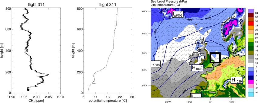
J. L. France et al.: North Sea methane 73
2.1 Aircraft capability nent, w, to approximately ±0.05 ms−1 . We assume for the
two horizontal wind components, u and v, similar high un-
The maximum range of the Twin Otter aircraft during the certainties due to aircraft movement. A detailed description
flight campaigns was approximately 1000 km. Although the of the Twin Otter turbulence instrumentation and associated
aircraft is capable of flying up to 5000 m altitude, most of the data processing can be found in Weiss et al. (2011).
flying was limited to below 2000 m; in regions with no mini- Ambient air temperature was observed with Goodrich
mum altitude limit, the aircraft could be flown at the practical Rosemount Probes, mounted on the nose of the aircraft.
limit of 15 m above sea level. The instrument fit included use A non-de-iced model 102E4AL and a de-iced model
of a turbulence boom, which limited the speed to a maximum 102AU1AG logged the temperature at 0.7 Hz. Atmospheric
of 140 kn (∼ 70 ms−1 ); throughout the campaigns, the target humidity was measured with a Buck 1011C cooled-mirror
aircraft speed for surveying was 60 ms−1 . The aircraft was hygrometer. The 1011C Aircraft Hygrometer is a chilled-
limited to a minimum safe separation distance of 200 m from mirror optical dew point system. The manufacturer stated a
any O&G production platforms. reading accuracy of ±0.1 ◦ C in a temperature range of −40
The total weight of the aircraft on take-off is limited to to +50 ◦ C. Chamber pressure and mirror temperature were
14 000 lb (6350 kg). Allowing for fuel and crew, this left recorded at 1 Hz.
2086 kg for the instrumentation. The total power available on
the aircraft is 150 A at 28 V, and inverters were used to pro- 2.3 In situ atmospheric chemistry instrumentation
vide 220 V to those instruments that required it. Altitude and
air speed were determined by static and dynamic pressure A Los Gatos Research (LGR) Ultraportable Greenhouse Gas
from the aircraft static ports and heated Pitot tube, logged Analyser (uGGA) was installed to measure CH4 , CO2 and
using Honeywell HPA sensors at 5 Hz. A radar altimeter H2 O. The expected manufacturer precision for the CH4 mea-
recorded the flight height at around 10 Hz. An OxTS (Oxford surement was < 2 ppb averaged over 5 s and < 0.6 ppb over
Technical Solutions) inertial measurement system coupled to 100 s. The response time of the LGR uGGA itself (i.e. the
a Trimble R7 GPS was used to determine the aircraft position flush time through the measurement cell) was over 10 s.
and altitude. This system gives all three components of air- To achieve higher-temporal-frequency data, a fast Picarro
craft position, altitude and velocity at a rate of 50 Hz. The G2311-f was installed to provide measurements of CH4 , CO2
chemistry inlets on the Twin Otter are similar to those fitted and H2 O at ∼ 10 Hz, with 1σ precision of ∼ 1ppb over 1 s
to the FAAM (Facility for Airborne Atmospheric Measure- for CH4 . A third greenhouse gas analyser, an LGR Ultra-
ments) BAe (British Aerospace) 146 large atmospheric re- portable CH4 /C2 H6 Analyser (uMEA) was used to measure
search aircraft (e.g. O’Shea et al., 2013) and were fitted with CH4 and C2 H6 . In-house laboratory measurements suggest
the inlet facing to the rear (Fig. A1). A single line (1/400 Syn- C2 H6 1σ precision at 1 s is ∼ 17 ppb for the LGR uMEA.
flex tubing) was taken from the inlet to a high-capacity pump During the 2019 airborne campaign, atmospheric C2 H6 was
with the instruments branching from this line. The aircraft also monitored by a tuneable infrared laser direct absorption
was fitted out during the week before each of the two flight spectrometer (TILDAS, Aerodyne Research Inc.) (Yacovitch
campaigns, allowing for significant changes to be made be- et al., 2014b) with an expected precision of 50 ppt (parts per
tween 2018 and 2019 based on instrument performance and trillion) for C2 H6 over 10 s. This instrument utilises a con-
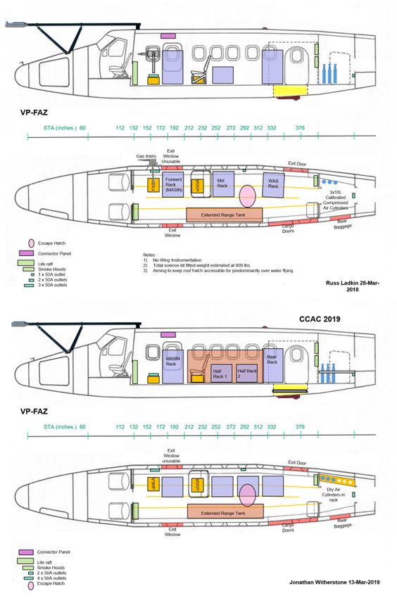
data from 2018 (Fig. 1). tinuous wave laser operating in the mid-infrared region (at
λ = 3.3 µm). A further description of the TILDAS instrument
2.2 Boundary layer physics instrumentation set-up and performance is available in the Appendices along
with instrument precisions and response times in Table A1.
A fast-response temperature sensor and a nine-hole NOAA
BAT “Best Air Turbulence” probe (Garman et al., 2006) were 2.4 Calibration of in situ instrumentation
mounted on a boom on the front of the aircraft (see photo,
Fig. A2). This instrumental set-up was chosen to reduce flow 2.4.1 CH4 and CO2 calibration
distortion effects by the aircraft. These fast-response mea-
surements of wind and temperature fluctuations were made In situ CH4 and CO2 instruments were calibrated in flight us-
with a frequency of 50 Hz. Garman et al. (2006) investigated ing a manually operated calibration deck, shown in schematic
the uncertainty of the wind measurements by testing a BAT form in Fig. 2. The calibration gases consisted of a suite
probe in a wind tunnel. They assessed that the precision of of WMO-referenced (World Meteorological Organization)
the vertical wind measurements due to instrument noise was standards with a “high”, “low” and “target” designation.
approximately ±0.03 ms−1 . Garman et al. (2008) showed The high CH4 concentration was ∼ 2600 ppb; low was
that an additional uncertainty in the wind data occurs when a ∼ 1850 ppb; and target was ∼ 2000 ppb. CO2 concentrations
constant up-wash correction value is used, as proposed by the were high at ∼ 468.5 ppm, low at ∼ 413.9 ppm and target
model of Crawford et al. (1996). We use the Crawford model, at ∼ 423.6 ppm. The absolute values of the cylinders varied
which increases the uncertainty in the vertical wind compo- between years as they were re-filled and re-certified to the
https://doi.org/10.5194/amt-14-71-2021 Atmos. Meas. Tech., 14, 71–88, 2021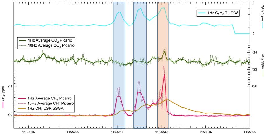
74                                                                                          J. L. France et al.: North Sea methane

Figure 1. Instrument schematics for the Twin Otter aircraft as deployed in 2018 and 2019, detailing changes in layout and instrumentation
between the two campaigns. The top panel is the 2018 fit, and the lower panel is the 2019 fit. VP-FAZ is the Twin Otter aircraft ID.
(1 in. = 2.54 cm; 1 lb = 0.45 kg.)

Atmos. Meas. Tech., 14, 71–88, 2021                                                        https://doi.org/10.5194/amt-14-71-2021
J. L. France et al.: North Sea methane                                                                                          75

NOAA WMO-CH4 -X2004A and WMO-CO2 -X2007 scales.                   flight contain a systematic altitude-dependent bias. However,
The calibration deck is designed so that upon the calibra-        as cabin pressure only affects the spectroscopic baseline, the
tion valve opening, the calibration gas flow rate is sufficient   zero offset of the measurements is affected but not the in-
to overflow the inlet. A similar approach to in-flight calibra-   strument gain factor. Therefore, as long as each plume mea-
tion is also applied on the NOAA WP-3D aircraft (Warneke          surement is referenced to a measured background at the same
et al., 2016). Full details of the calibration procedure are      altitude, this cabin pressure sensitivity does not significantly
recorded in the Appendices. CH4 uncertainty (1σ ) is calcu-       impact the calculated C2 H6 mole fraction enhancements. As
lated from the in-flight target gas measurements as 1.24 ppb      stated above, future deployments will mitigate this issue by
for the Picarro G2311-f and 1.77 ppb for the uGGA, giving         employing in-flight calibration cylinders that are certified for
performance comparable with similar instrumentation on the        C2 H6 . The potential to use a fast, frequent calibration for
FAAM aircraft (O’Shea et al., 2014). The excellent agree-         baseline correction as described by Gvakharia et al. (2018)
ment between measured and expected values of CH4 for the          and Kostinek et al. (2019) will also be investigated, although
target cylinder (for the Picarro and uGGA) gives us confi-        this has payload implications, as it requires an extra calibra-
dence in being able to operate to high levels of accuracy with    tion cylinder. Alternatively, the optical bench could be re-
a very limited period of instrument fitting and testing. CO2      engineered to sit within a hermetically sealed pressure vessel,
uncertainty (1σ ) at 1 Hz is calculated as 0.20 ppm for the Pi-   as described by Santoni et al. (2014).
carro G2311-f and 0.35 ppm for the uGGA. More details on
the calibration and associated uncertainties are shown in the     2.5     Spot sampling
Appendices.
                                                                  Manually triggered spot sampling provides a cost-effective
2.4.2   C2 H6 calibration                                         and relatively simple sample collection method to allow for
                                                                  analyses which cannot be performed mid-flight or require
The calibration cylinders installed on the Twin Otter dur-        specialist laboratory facilities to gain useful levels of pre-
ing both campaigns did not contain measurable amounts of          cision. Two discrete air-sampling systems were used dur-
C2 H6 , and therefore in-flight calibrations could not be per-    ing these flights to enable post-flight analysis for VOCs and
formed. This represents a limitation on the accuracy and          δ 13 CCH4 .
traceability of the C2 H6 measurements during these cam-
paigns and will be addressed for future studies using the         2.5.1    Son of Whole Air Sampler (SWAS)
BAS Twin Otter. The uMEA was calibrated in the labora-
tory post-campaign for the 2018 campaign and pre- and post-       The Son of Whole Air Sampler (SWAS) is a new, updated
campaign in the laboratory for the 2019 season. The uMEA          version of the parent WAS system fitted to the FAAM BAe
instrument cavity is not temperature stabilised, resulting in     146 large atmospheric research aircraft (e.g. as used by
significant measurement drift during the course of operation.     O’Shea et al., 2014), which it is designed to supersede. The
Corrections for C2 H6 and CH4 measurement drift as a func-        system comprises a multitude of inert Silonite-coated (En-
tion of cavity temperature were determined experimentally         tech) stainless steel canisters, grouped together modularly in
by analysing two calibration cylinders alternately over the       cases with up to 16 canisters per case. Onboard the Twin Ot-
course of several hours as the cavity temperature increased.      ter, two cases can be fitted allowing for up to 32 canisters to
These corrections were then applied to the uMEA C2 H6 and         be carried per flight. The theory of operation is to capture dis-
CH4 measurements obtained from both the 2018 and 2019             crete air samples from outside of the aircraft and compress
flight campaigns.                                                 the sample either into 1.4 or 2 L canisters at low pressure
   The TILDAS (deployed in 2019) measures a water line,           (40 psi; 275 kPa) via pneumatically actuated bellows valves
allowing for measurements to be corrected to dry mole using       (PBVs, Swagelok BNVS4-C). Full details of the operation
the TDLWintel software (Nelson et al., 2004) to account for       of SWAS are included in the Appendices. For the 2019 cam-
changes in humidity during the flight (as discussed in Pitt       paign, SWAS was updated with the addition of 2 L flow-
et al., 2016). The raw measured data were calibrated pre-         through canisters, making narrow plumes easier to capture
and post-flight using two cylinders of a known concentra-         due to reduced sample line lag and fill times.
tion, whose mole fractions spanned the measurement range             SWAS canister sampling was manually triggered during
observed during flights for C2 H6 . By assuming a linear rela-    the flights according to in situ observations made by fast-
tionship, the calibrated mole fraction corresponding to each      response instrumentation of CO2 , C2 H6 and CH4 , with the
measured TILDAS mole fraction was given by interpolating          aim of capturing specific oil and gas plumes. The samples
the scale between the pre- and post-flight calibration refer-     were analysed at the University of York for VOCs post-
ence points. Previous studies have reported the sensitivity of    flight using a dual-channel gas chromatograph with flame
TILDAS systems to aircraft cabin pressure (Gvakharia et al.,      ionisation detectors (Hopkins et al., 2003). Firstly, 500 mL
2018; Kostinek et al., 2019; Pitt et al., 2016). This sensitiv-   aliquots of air are withdrawn from the sample canister and
ity means that the C2 H6 mole fractions measured during the       dried using a condensation finger held at −30 ◦ C; then they

https://doi.org/10.5194/amt-14-71-2021                                                    Atmos. Meas. Tech., 14, 71–88, 2021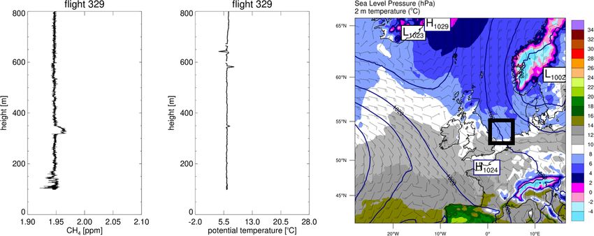
76 J. L. France et al.: North Sea methane
Figure 2. Layout of the plumbing of the calibration system (and inlet system) for the 2018 campaign.
are pre-concentrated onto a multi-bed carbon adsorbent trap gain a meaningful source δ 13 CCH4 signature (e.g. Rella et
consisting of Carboxen 1000 and Carbotrap B (Supelco) and al., 2015).
transferred to the gas chromatography (GC) columns (Al2 O3 ,
NaSO4 deactivated and open tubular; PLOT – porous layer,
open tubular) in a stream of helium. Chromatogram peak 3 Overall approach to flight planning
identification was made by reference to a calibration gas
standard containing known amounts of 30 VOCs rang- The majority of flights were conducted during good operat-
ing from C2 to C9. Compounds of interest include C2 H6 , ing conditions, i.e. daytime, no precipitation, clear or broken
propane, butanes, pentanes, benzene and toluene; a full list is cloud, winds < 10 ms−1 , and visibility, to allow for flying
shown in Table A2. at a minimum safe altitude around the task area. Two ap-
proaches were trialled to assess CH4 emissions from offshore
2.5.2 FlexFoil bag sampling gas installations: (i) regional survey and (ii) specific plume
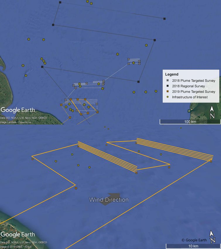
sampling. The flight modes are demonstrated in Fig. 3, with
Spot sampling for δ 13 CCH4 by collecting whole-air sam- the dark-grey pattern showing a flight plan for regional mea-
ples into FlexFoil bags (SKC Ltd) has been in use on both surements and the orange and white patterns demonstrating
the FAAM BAe 146 research aircraft (e.g. Fisher et al., specific plume sampling flight patterns. Flight plans to sam-
2017) and during ground-based mobile studies (e.g. Lowry ple specific installations were designed to capture a full range
et al., 2020) and provides a relatively cost-effective and rapid of expected emissions using the UK National Atmospheric
methodology for sample collection. The method does have Emissions Inventory (NAEI) as a guide.
some limitations, however, as the FlexFoil sample bags are Regional survey intentions were twofold: firstly, to offer
only stable for a number of compounds (including CH4 ). an identification process for emitters of interest that could
Samples captured in both FlexFoil bags and SWAS were specifically be targeted for plume sampling modes and, sec-
measured at Royal Holloway using continuous-flow isotope ondly, to build a picture of aggregate bulk emissions for mul-
ratio mass spectrometry (CF-IRMS; Fisher et al., 2006), and tiple upwind platforms. This method has been successfully
each measurement has a δ 13 CCH4 uncertainty of ∼ 0.05 ‰. employed during a Gulf of Mexico airborne study (Gorchov
Each sample is also measured for CH4 mole fraction us- Negron et al., 2020). However, in the work presented here,
ing cavity ring-down spectroscopy to allow for direct com- regional surveys were poor for identifying plumes (being too
parison to in-flight data (Fig. A3). Alternative, continuous far downwind of platforms or not intercepting thin filament
in-flight δ 13 CCH4 instrumentation currently cannot replicate layers containing CH4 enhancements), and attempts to aggre-
the precision of laboratory sampling, and the few seconds gate bulk emissions were hindered by the often encountered
of enhanced CH4 that would be encountered during flight is complex boundary layer structure over the area, which con-
not sufficient for averaging of continuous δ 13 CCH4 data to trolled dispersion of CH4 emissions from rigs. From the re-
Atmos. Meas. Tech., 14, 71–88, 2021 https://doi.org/10.5194/amt-14-71-2021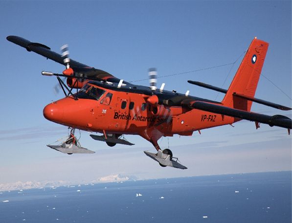
J. L. France et al.: North Sea methane                                                                                                  77

                                                                           approximately 260 m to capture the entire extent of a down-
                                                                           wind plume. Plume dispersion was dependent on meteorol-
                                                                           ogy and emission type (venting, fugitive or combustive emis-
                                                                           sions), and as such, maximal plume heights varied between
                                                                           individual pieces of infrastructure. Upwind transects were
                                                                           flown at a median height between the minimum and maxi-
                                                                           mum stacked runs.

                                                                           4     Assessing and addressing issues encountered during
                                                                                 flights

                                                                           A number of issues were encountered during the flights that
                                                                           influenced the measurements made. An initial presentation
                                                                           of these issues is given here, with recommendations for im-
                                                                           provements given in Sect. 6 below.

                                                                           4.1    Complex marine boundary layers

                                                                           Boundary layer structure proved to be a important influence
                                                                           on observed CH4 mixing ratios. Figure 4 shows the measured
                                                                           profiles of CH4 (left-hand panel) and potential temperature
                                                                           (right-hand panel) during an offshore flight in April 2018
                                                                           along with the corresponding synoptic chart. Potential tem-
Figure 3. The top panel shows flight patterns of the regional and          perature was calculated as described by Stull (1988). The
plume capture styles of flight deployed between 2018 and 2019,
                                                                           potential temperature profile demonstrates that the bound-
alongside infrastructure of interest (such as drilling rigs, gas distri-
bution platforms or production platforms). The bottom panel shows
                                                                           ary layer structure on this day (and many other days) was
a 2019 plume sampling survey of idealised stacked transects in the         partly stable stratified, showing mostly an increase in poten-
2D plane downwind of infrastructure of interest. © Google Earth            tial temperature with height, and the boundary layer showed
2019 for background imaging.                                               complex layering. The prevailing meteorological situation at
                                                                           that time, illustrated by the synoptic chart in Fig. 4, was of a
                                                                           persistent anticyclonic ridge, stretching from the south-west
gional flight data derived in 2018 and considering the work in             over the British Isles and western Europe, with associated
other offshore studies in this area (e.g. Cain et al., 2017), the          low wind speeds and poorly defined airflow over the south-
regional flight mode was determined to be of limited scien-                ern North Sea sector. The observed layering was partly also
tific value in the context of this project, and this flight pattern        caused by residual boundary layers from previous days and
was not used during the 2019 campaign.                                     nights which had not dispersed. The structure of the bound-
    Plume sampling flights were conducted in both 2018 and                 ary layer in Fig. 4 clearly had an important influence on the
2019. These flights involved the use of a box pattern to                   vertical profile of CH4 , which varied and shows a complex
create both upwind and downwind transects on either side                   profile with height. Due to the complexity of the bound-
of the infrastructure of interest. Upwind transects provided               ary layer structure, it was concluded that it would be in-
an understanding of other methanogenic sources (such as                    appropriate to use a particle dispersion model such as the
other installations, ships or long range transport of air masses           Numerical Atmospheric-dispersion Modelling Environment
from onshore sources) that could interfere with observed                   (NAME) (Jones et al., 2007) to derive a bulk regional emis-
CH4 plumes downwind and were conducted to be confident                     sion estimate. The impact of the residual layers of CH4 en-
that plumes were solely originating from the targeted infras-              hancement make in-flight decisions very challenging for two
tructure. Vertically stacked downwind transects at a distance              main reasons: (i) it is difficult to determine which enhance-
of 1 to 10 km away from emission sources were conducted                    ments are from installations and require further investigation,
to better capture the vertical extent of the plume in a 2D                 especially if flying at some distance downwind from a poten-
Lagrangian plane for CH4 flux quantification using mass                    tial source or on a regional survey pattern, and (ii) emissions
balance analysis (e.g. O’Shea et al., 2014). The vertically                being actively released can become trapped in vertically thin
stacked transects in profile, as planned from the 2019 field               filaments, which can be easily missed when flying stacked
deployment, are demonstrated in Fig. 3. The separation be-                 legs, depending on flight altitude. In contrast, on days with
tween vertically stacked transects was usually 60 m with a                 a well-mixed boundary layer the CH4 profile stays relatively
minimum absolute height of 45 m above sea surface up to                    constant with height and shows an increase only near a CH4

https://doi.org/10.5194/amt-14-71-2021                                                            Atmos. Meas. Tech., 14, 71–88, 2021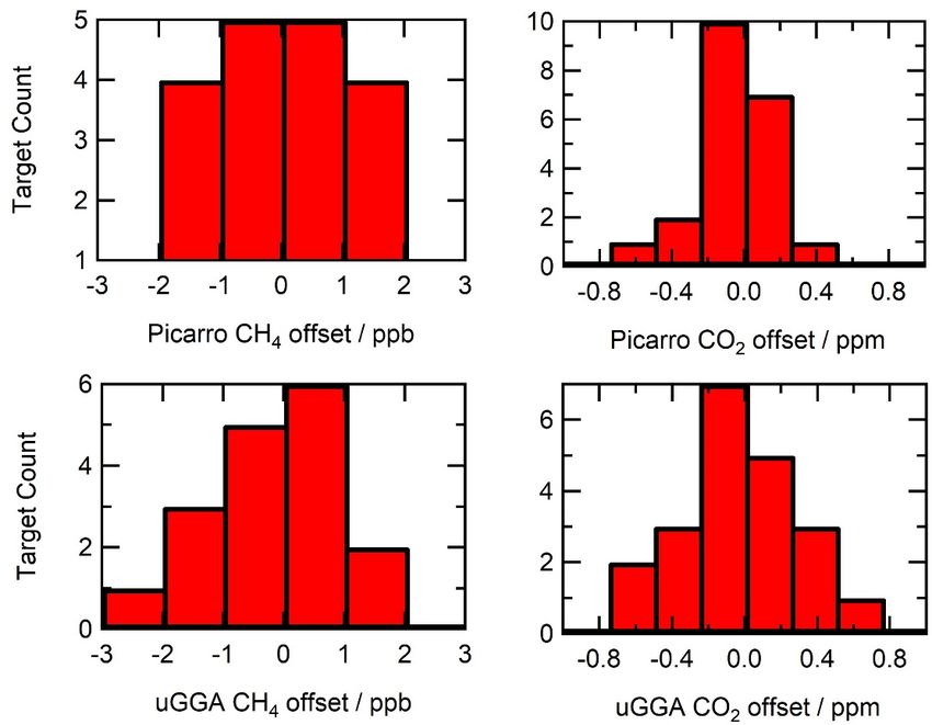
78 J. L. France et al.: North Sea methane
source. Figure 5 shows an example of CH4 and potential tem- increased the success of capturing plumes (Fig. A3). The im-
perature profiles, in a well-mixed boundary layer during a provements included modified flight planning, with an in-
flight in May 2019; the synoptic situation on that day was creased number of passes through discovered plumes. This
consistent with a slow-moving cyclonic south-easterly air- approach resulted in increased fuel consumption per plume
flow. It can clearly be seen how the potential temperature and but contributed to the higher success rate of plume capture.
CH4 profiles stay almost constant with height and only show The comprehensive update to the SWAS system, which in-
structure when intercepting a CH4 emission at 300 to 350 m cluded continuous sample throughflow allowed for more pre-
altitude. The potential temperature profile indicates neutral cise spot sampling to be achieved.
stratification of the boundary layer.
4.2 Instrument response times 5 Creation of data products
5.1 Methane fluxes
The role of the continuous in-flight measurements is to pro-
vide the backbone of the dataset and ensure that, at a bare A methane flux can be calculated from the CH4 mixing ratio
minimum, the flights are able to identify areas of CH4 en- data using mass balance techniques (e.g. O’Shea et al., 2014;
hancement and inform on the likely sources of the CH4 en- Pitt et al., 2019) in which a vertical 2D plane is defined at a
hancement, hence the decision to run redundancy measure- fixed distance downwind of the infrastructure of interest, and
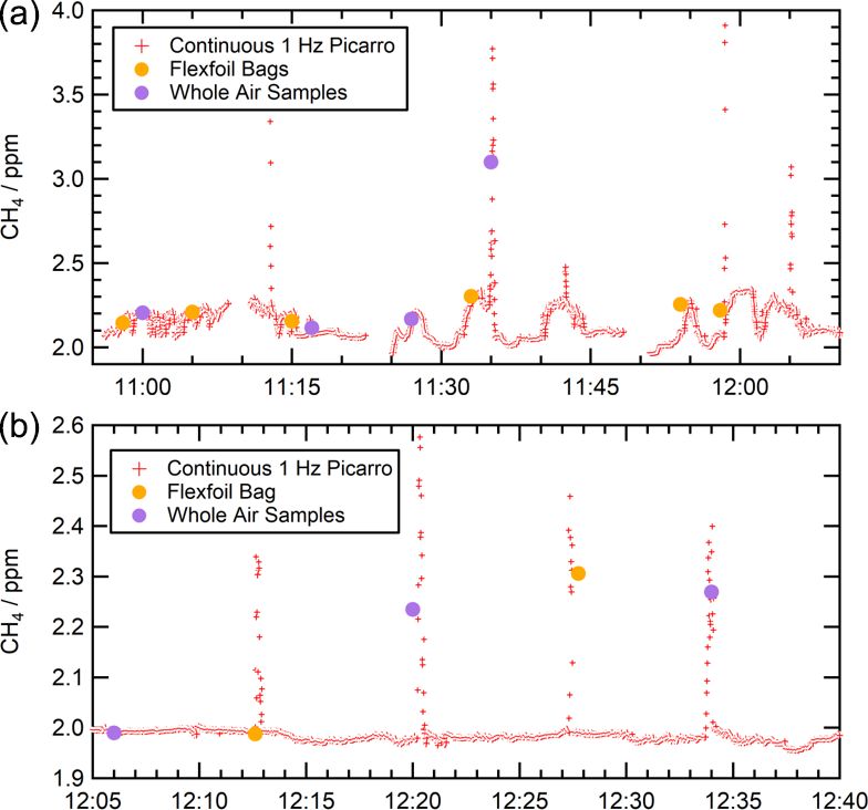
ments of CH4 utilising an LGR uGGA. Figure 6 shows typ- sampling is conducted across the stacked transects at this dis-
ical instrument responses to a CH4 plume, and it is clear tance if a plume is identified in the downwind plane. Fluxes
that the cell turnover time of the uGGA is not sufficient to were derived using Eq. (1):
capture the fine detail of the plume. Whilst the uGGA and
uMEA are capable of determining the whole infrastructure
Flux = Xplume − Xbackground × nair × V × 1x × 1z, (1)
mass balance and average infrastructure ethane–methane ra-
tios, the refined understanding of the true plume is lost in where Flux is the bulk net flux passing through the x − z
these slower response instruments. This is important, as the plane per unit time, nair is the molar density of air (mol m−3 ),
combined Picarro G2311-f and TILDAS data can detect sev- Xplume is the average CH4 mole fraction measured within the
eral sources from the same installation (Fig. 6) because of plume and Xbackground is the CH4 mole fraction of the back-
their rapid measurement cell turnover. This information can ground. V is the wind component perpendicular to the flight
be used to infer either cold venting (CH4 and C2 H6 ) or com- track; 1x is the plume width perpendicular to the upwind–
bustion from flares or generators (CO2 , CH4 and C2 H6 ), downwind direction; and 1z relates to the vertical extent of
which could then be used to determine CH4 emission factors the plume.
from identified flares (Gvakharia et al., 2017). The CH4 and CO2 measurements from the 10 Hz response
There are a number of other implications that arise from instruments were used to provide the highest accuracy in the
slow measurement response. For example, in-flight spot sam- (i) lateral plume width and (ii) number of unique plumes
pling requires guidance from fast-response instruments that identified from each individual platform. Slower-response in-
can indicate the optimum timing to collect samples that span struments would allow for flux calculations but would not
the plume and thereby capture the representative chemical be able to identify individual plumes from the same plat-
nature of the plume. Further, in-flight calibrations must be form. This could be useful to distinguish, for example, mul-
matched to the slowest-response instrument to ensure stabil- tiple plumes from different emission processes that are spa-
isation of the measurement of calibration gases across all in- tially distinct within the same platform (e.g. a fugitive source
struments. Although useful from a cross-checking purpose, versus a flare). A background mixing ratio was selected to
use of slower-response instruments can introduce additional, best represent the conditions observed during the flight at
unwanted loss of measurement time and excessive use of the specific time of survey. An average of 30 s of data from
calibration gases, and the benefits of instrument redundancy either side of the plume on each run were used if this was
should be carefully considered. deemed appropriate with a clean upwind sampling leg. When
the upwind sampling was contaminated, more caution should
4.3 Spot sampling improvements between the 2018 and be taken when selecting an appropriate background so that
2019 campaigns the background value is not distorted by extraneous far-field
sources.
In-flight spot sample collection was carried out during both For the flux analysis, a flux across each individual stacked
the 2018 and 2019 campaigns. Such sampling is challeng- horizontal run downwind of a plume was calculated be-
ing and requires fast-response instruments to be viewable to fore scaling in the vertical component. The flux was then
the operator to give the best chance of collecting samples integrated across potential minimum and maximum plume
at appropriate points across the plumes. For 2019, a num- depths. Figure 7 (upper panel) represents a reduced vertical
ber of simple adaptations were introduced that significantly resolution of the plume where transects at intermediate alti-
Atmos. Meas. Tech., 14, 71–88, 2021 https://doi.org/10.5194/amt-14-71-2021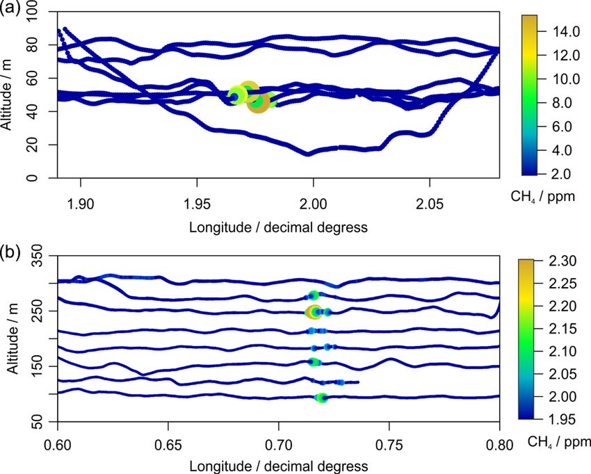
J. L. France et al.: North Sea methane                                                                                                   79

Figure 4. Example of CH4 and potential-temperature profiles showing the large amount of structure arising from residual boundary layers.
The increase of the potential temperature with height shows stable stratification of the boundary layer. The synoptic chart over the eastern
North Atlantic and north-western Europe shows contoured sea level pressure (hPa), 2 m temperature (◦ C, right-hand side colour scale) and
wind for 20 April 2018 12:00 UT and reveals relatively low wind speeds and poorly defined airflow over the southern North Sea sector,
allowing for the build-up of residual boundary layers. Synoptic chart image produced by the UK National Centre for Atmospheric Science
(NCAS) using Weather Research and Forecasting model WFR-ARW (Advanced Research WRF) version 3.7.1, with a 20 km grid spacing and
51 vertical levels initialised using the NOAA Global Forecast System. NCAS (National Centre for Atmospheric Science) Weather Research
Catalogue (https://sci.ncas.ac.uk/nwr/pages/home, last access: 6 November 2020). The black rectangle approximates the survey region.

Figure 5. Example of CH4 and potential-temperature profiles in a well-mixed boundary layer under neutral conditions. The potential temper-
ature and CH4 profiles stay relatively constant and CH4 shows only an increase in the surface layer and when intercepting an enhancement
at 300 to 350 m height. The synoptic chart for 6 May 2019 12:00 UT shows a cyclonic south-easterly airflow over the southern North Sea
sector originating from the Benelux region. The black rectangle approximates the survey region over open water.

tudes through the plume were not conducted. In this case, the           the upper limit of the plume was selected as the atmospheric
minimal plume depth is the narrow span captured by observa-             marine boundary layer. The greatest uncertainty in bulk flux
tion in the 45.9–51.9 m altitude window. The maximal plume              arises when the vertical extent of the plume is not fully cap-
depth is taken as the height difference between the highest             tured. For the 2019 campaign, the flux uncertainty related to
and lowest transects without CH4 enhancements, which are                plume depth was reduced by a factor of 10 compared to the
above and below the plume, respectively; this value has to              2018 campaign (as seen in Table 1) by completing a rigor-
be used as the maximum due to incomplete sampling of the                ous set of stacked transects at multiple heights throughout
void area seen in the upper panel of Fig. 7. In cases where the         the plume. The fluxes presented here serve to demonstrate
base and top of the plume were not sampled (e.g. during 2018            the approach and the impact of sampling strategy and mete-
sampling), the lower limit was selected as the sea surface, and         orological conditions on the calculation. Flux estimates for

https://doi.org/10.5194/amt-14-71-2021                                                           Atmos. Meas. Tech., 14, 71–88, 2021
80                                                                                         J. L. France et al.: North Sea methane

Figure 6. A cross section of CH4 , CO2 and C2 H6 measurement response during one plume sample as recorded by Picarro G2311-f in pink
and green (10 Hz as dashed lines and downsampled to 1 Hz as solid lines), TILDAS 1 Hz in cyan and Los Gatos uGGA 1 Hz in brown.
The difference between the uGGA and Picarro at 1 Hz arises from the slower uGGA response time is due to the slower cell turnover. The
blue-shaded area shows enhancement in C2 H6 and CH4 , indicating cold venting; the orange-shaded area shows enhancement in C2 H6 , CH4
and a small amount of CO2 potentially indicating a co-located combustion source.

                                                                      Table 1. A comparison of flux lower and upper bounds for two indi-
                                                                      vidual example plumes across each year of survey as scaled by the
                                                                      vertical resolution available. The plumes themselves are not compa-
                                                                      rable, but the method changes demonstrate the increased certainty
                                                                      in the final results.

                                                                               Survey      CH4 flux lower      CH4 flux upper
                                                                               year       bound (kT yr−1 )    bound (kT yr−1 )
                                                                               2018                   1.83                17.9
                                                                               2019                   0.67                1.04

                                                                      5.2   Ethane–methane ratios (C2 : C1) as a source tracer

                                                                      It has already been well established that continuous C2 H6
                                                                      measurements can be an excellent diagnostic tool for ascrib-
                                                                      ing enhancements of co-located CH4 and C2 H6 to natural
Figure 7. Plumes measured from separate installations to demon-
strate the differences in strategies between 2018 and 2019.
                                                                      gas emissions in both urban areas (e.g. Plant et al., 2019),
(a) Plume sampled downwind with poorer vertical spatial resolu-       semi-rural areas (e.g. Lowry et al., 2020) and during large-
tion in the 2D plane during the 2018 portion of the campaign. CH4     scale evaluations of oil and gas fields from aerial studies in
measured values are much higher due to platform activities during     the USA (e.g. Peischl et al., 2018), Canada (Johnson et al.,
the survey time. (b) Plume sampled downwind in 2019 with inter-       2017) and the Netherlands (Yacovitch et al., 2018). During
mediate transects enabling higher vertical spatial resolution. Note   this work, two methods were used to establish C2 H6 –CH4
that the colour scale across each plot signifies different measured   ratios (hereafter, described as C2 : C1). In 2018 the LGR
CH4 ; the scales on the upper and lower plots are different.          uMEA was used to measure C2 H6 –CH4 ratios. The bene-
                                                                      fits of such instrumentation are in its simplicity of operation
                                                                      and that few considerations are required for corrections or
all sampled platforms will be presented in a future study, in-        variable lags, as both species are measured at the same rate
cluding a full treatment of component uncertainties.                  and within the same optical cavity. C2 : C1 can therefore be
                                                                      readily determined as the gradient of a linear regression be-

Atmos. Meas. Tech., 14, 71–88, 2021                                                        https://doi.org/10.5194/amt-14-71-2021
J. L. France et al.: North Sea methane 81
tween the C2 H6 and CH4 measurements. However, the low Where repeat transects were conducted at different altitudes,
sensitivity to C2 H6 (standard deviation of > 10 ppb in C2 H6 this made selection of appropriate background samples for
over 10 s of background flying) only allowed emissions from Keeling plots challenging, since the background CH4 mix-
two platforms to be characterised for C2 : C1 ratios during ing ratio and δ 13 C varied over the different altitudes. This be-
the whole of the 2018 campaign and none during 2019 using comes particularly detrimental to Keeling plot validity where
the LGR uMEA method. the range in sampled emission mixing ratios is small, since
In 2019 the addition of the TILDAS 1 Hz C2 H6 instru- uncertainty in the background samples then becomes more
ment allowed for better precision of C2 H6 (< 1 ppb) with important.
a faster flush time in the measurement cell. The C2 H6 data In Fig. 8, a sensitivity analysis is presented from one of
are time-matched with the 1 Hz Picarro CH4 dataset to allow the flights investigating the effect of reducing the number of
C2 : C1 derivation. As the instruments do not have the exact samples on the uncertainty in the δ 13 CCH4 source signature
same flow rate and different cell residence times, the C2 : C1 determined for a plume. In this case nine samples were col-
ratios were determined using the integral of each CH4 and lected, but this took place over eight downwind transects and
C2 H6 enhancement using Gaussian peak fitting. A compari- one upwind transect of a cluster of installations, which is not
son between the 2018 flight, 2019 flight and published data feasible to repeat for sampling large numbers of installations.
derived from the same geographical area is shown in Ta- As shown in Fig. 8, the uncertainty in the δ 13 CCH4 source
ble 2. Although both instruments have been operated for this signatures increases only slightly with a reduction in num-
work without in-flight calibration or engineering solutions ber of sampling points, with the exception of one n = 3 run
to address cabin-pressure-sensitivity issues (Gvakharia et al., where the source signature is poorly defined. A minimum of
2018) due to weight and time constraints, the agreement be- three data points can therefore be sufficient for classifying a
tween years and with published expected values is highly re- source of CH4 emissions (such as thermogenic, microbial or
assuring. The added value in high-precision C2 : C1 demon- pyrogenic sources), providing that the background and point
strates that C2 H6 is not just a tracer for matching emissions to samples are captured with a large enough range of CH4 con-
natural gas; it can give information as to proportions of emis- centration and providing that there is no mixing of sources.
sions from mixed sources (as previously used by Peischl et This will typically require collection of more than three sam-
al., 2018) or can be used to identify a likely emission point in ples, given some may miss the targeted plumes or potentially
a process chain depending upon enrichment or depletion of be lost during storage or processing as aforementioned. Al-
C2 H6 relative to CH4 . The inclusion of a continuous instru- though a two-point Keeling plot is technically possible, it is
ment with a level below parts per billion (sub-ppb) of detec- impossible to gauge the quality of the regression to be sure
tion for C2 H6 is considered vital for future work with ther- that only a single source has been captured.
mogenic sources of CH4 to allow for more precise source at-
tribution of emissions where no spot sampling has occurred.
6 Conclusions
5.3 δ 13 CCH4 for CH4 source attribution
Given the restrictions and time constraints on the science
The principal method of δ 13 CCH4 source characterisation flights, important lessons for offshore oil and gas airborne
utilises the principles outlined by Keeling (1961) and Pataki measurement campaigns have been learned for rapid instru-
et al. (2003) and has been well utilised since to create ment re-fitting and agile deployment of a small aircraft for fu-
δ 13 CCH4 databases for a plethora of known CH4 sources (e.g. ture campaigns. A key finding from this study is that offshore
Sherwood et al., 2017). In order for a Keeling plot to give meteorological conditions define the ability of the flights to
useful results to determine a δ 13 CCH4 source signature of produce valuable data and suitable meteorology with a well-
a CH4 emission, the emission must have been successfully mixed (neutral) boundary layer is critical to deriving a re-
captured multiple times and with a range of CH4 mixing ra- gional emission estimate through regional modelling. Flying
tios (which could be achieved by passes at different distances in conditions with multiple residual boundary layers makes
or heights downwind of a point source). This sampling pro- interpretation difficult and pin-pointing emissions especially
cess takes time (especially on an aircraft), where the emis- challenging, as emission plumes can easily be missed when
sion plume is only intercepted once per transect and time in they are trapped in thin filaments, increasing the uncertainties
the plume is limited so that only one spot sample can be taken of measurement-based emission flux calculations. Although
whilst “in-plume”. Beyond the time limitations, sampling of not possible for this work given aircraft scheduling, it is rec-
a range of CH4 mixing ratios from emissions and appropri- ommended that offshore observations are scheduled with a
ate background samples is not straightforward. Background long window of opportunity to ensure optimal flying condi-
sampling must capture the air into which emissions are re- tions. Predictions of the likelihood of a residual boundary
leased, but during flights the meteorological conditions of- layer over a coastal area could be achieved through high-
ten resulted in significant variation of CH4 mixing ratios and spatial-resolution forecast models such as the UK Met Of-
δ 13 CCH4 with altitude, in addition to horizontal variations. fice forecast model (Milan et al., 2020). Information on the
https://doi.org/10.5194/amt-14-71-2021 Atmos. Meas. Tech., 14, 71–88, 202182 J. L. France et al.: North Sea methane
Table 2. Reported data for C2 : C1 for a single installation surveyed during both the 2018 and 2019 surveys. Well data from UK oil and
gas authority report are available at https://dataogauthority.blob.core.windows.net/external/DataReleases/ShellExxonMobil/GeochemSNS.
zip (last access: 7 January 2020) alongside measured C2 : C1 for CH4 enhancements measured during flights in the same geographic area.
Instrument(s) Method C2 : C1 Uncertainty
2018 flight Los Gatos ultraportable CH4 /C2 H6 Linear regression 0.029 ±0.014
2019 flight TILDAS C2 H6 and Picarro G2311-f CH4 Plume area integration 0.029 ±0.003
Published well data 0.031 ±0.009
Figure 8. (a) Keeling plot determined using nine samples collected around one installation, assumed to be the single source of excess CH4 .
(b) An illustration of the variation in δ 13 CCH4 source signature and its uncertainty determined by Keeling plot analyses for reduced sample
sizes. Each analysis represents a single Monte Carlo experiment with the original data, reducing the number of data points to the sample size
indicated at random; the δ 13 CCH4 source signature is then calculated with the remaining sample points. Error bars are 2 times the standard
error.
temperature structure over the previous few days using all For mass balance flux calculations, an emission plume and
the assimilated information, such as tephigrams and synop- the surrounding background variation in the species of in-
tic charts, would help determine the likelihood of residual terest, alongside local meteorology, must be fully resolved
boundary layers versus a simpler stratified, well-mixed layer. during the observation stage. This includes instruments with
For methods using alternative platforms such as ships or appropriate response times to fully capture the plume and
drones, coincidental measurements of vertical profiles must identify any internal structure that may suggest a mixed
be made to capture the true nature of the emission plume in source. An upwind leg must be conducted to ensure the
the current meteorology. plume and background are not contaminated by extraneous
Due to the size of the aircraft, payload restrictions and far-field sources, and the plume must be significantly dis-
power limitations demand challenging decisions for instru- tinct from this background for meaningful flux calculations.
ment selection. We recommend deploying at least one in- The plume must be laterally and vertically resolved in the
strument measuring CH4 (and CO2 ) at 10 Hz, allowing sev- 2D plane as much as possible at a fixed distance downwind
eral plumes emitted from a single installation to be resolved of the source. Straight and level runs must extend to either
(Fig. 6). Priority should next be given to a C2 H6 instrument side of the plume, and the vertical resolution must include
capable of a sub-ppb limit of detection at 1 Hz (or higher) multiple stacked transects with an identification of the top
in order to give certainty to the source of the CH4 emission. and bottom of the plume (where feasible) to reduce uncer-
Using C2 : C1 appears to be the simplest method for source tainty in the plume bulk net flux. Full understanding of the
attribution and is robust for distinguishing natural gas emis- meteorology with meteorological measurement instrumenta-
sions, where the gas has an C2 H6 component (Lowry et al., tion and a complete profile to determine characteristics of the
2020; Plant et al., 2019). Spot sampling is challenging, pay- marine boundary layer from the top to the surface, including
load heavy and time consuming, as several passes are needed determination of inversion heights, must be conducted during
to collect enough samples (especially for δ 13 CCH4 source at- the flight day when appropriate radiosonde soundings are not
tribution). However, results can be very informative, such as available. The observed impact of complex boundary layer
the ability to distinguish between a gas leak and a geological dynamics on plume dispersion also highlights an important
reservoir from depth or a near-surface reservoir (Lee et al., limitation of ship-based plume measurements, which are un-
2018). The improvements to SWAS, allowing for continuous able to resolve the vertical structure of the plume and there-
throughflow, has increased the success rate of peak sampling fore rely on the assumption of idealised models of plume dis-
but still relies on accurate user triggering. persion.
Atmos. Meas. Tech., 14, 71–88, 2021 https://doi.org/10.5194/amt-14-71-2021J. L. France et al.: North Sea methane 83
Appendix A
A1 TILDAS data processing and performance
The TILDAS data were processed as follows. Rapid tuning
sweeps of the laser frequency (2996.8 to 2998.0 cm−1 ) by
varying the applied current result in the collection of thou-
sands of spectra per second, which are co-averaged. The
resulting averaged spectrum is processed at a rate of 1 Hz
using a non-linear least-squares fitting algorithm to deter-
mine mixing ratios within the operating software, TDLWin-
tel (© Aerodyne). Averaging of these spectra and the path
length of 76 m achieved using a Herriott multipass cell pro-
vide the sensitivity required for trace gas measurement. Con-
tinuously circulated fluid from the Oasis chiller unit is used
as a heat sink for the thermodynamically cooled components,
and a flow interlock cuts power to the relevant components Figure A1. Photo of the rear-facing chemistry inlets on the BAS
if the coolant flow stops. Other optical components of the in- Twin Otter aircraft.
strument include a 15× Schwarzschild objective in front of
each laser, a germanium etalon for measuring the laser tuning
rate, a reference gas cell containing air at 25 Torr and numer-
ous mirrors for adjusting the laser beam alignment. During
the airborne campaign the instrument was operated remotely
via an Ethernet connection. The TILDAS C2 H6 instrument
accuracy has been tested against two standards containing
C2 H6 in mixing ratios of 39.79±0.14 ppb and 2.08±0.02 ppb
(high-concentration standard and target gas, respectively). As
the TILDAS technique relies on highly precise alignment of
the focussing and beam-alignment optics before and after the
multipass measurement cell, it is particularly prone to motion
that applies torque to the optical bench. To remove measure-
ment artefacts associated with this sensitivity, all data col-
lected for roll angles greater than 20◦ have been flagged.
The presence of the TILDAS in the 2019 campaign ruled out
using the multiple circular pass method around a potential
emission source as developed by Scientific Aviation for in- Figure A2. Photo of the BAS Twin Otter showing the turbulence
stallation emission flux measurements (Conley et al., 2017), boom protruding from the front of the aircraft superstructure.
as there was a risk of invalidating data due to the roll angle
of the plane if circling tightly around an installation.
The typical duration of calibration cylinder measurements
A2 CO2 and CH4 calibration during the 2018 campaign was 45 s. The Picarro G2311-f
analyser had a high flow rate of ∼ 5 SLPM (standard litre per
The three cylinders were sampled periodically in flight to de- minute), resulting in rapid flushing of both the inlet tubing
termine the instrument gain factor (slope) and zero offset for and sample cavity. The measured value for each calibration
each analyser. These parameters were linearly interpolated was taken as the average over 15 s prior to the calibration end,
between calibrations and used to rescale the raw measured as this allowed sufficient time for the measured value to reach
data (for further details see Pitt et al., 2016). The uncertain- equilibrium. The uGGA and uMEA both had much lower
ties associated with instrument drift and any instrument non- flow rates of ∼ 0.5 SLPM, resulting in a much longer equili-
linearity were assessed by sampling the target cylinder mid- bration time. Consequently, the calibration duration was not
way between high–low calibrations. The raw target cylinder of sufficient length for the uGGA and uMEA measurements
measurements were rescaled as per the sample data; the mean to reach equilibrium, and their calibration routine was com-
offset of these target measurements from the WMO-traceable promised. For these instruments each calibration run was fit-
cylinder value (and associated standard deviations) are given ted to an offset exponential function in an attempt to predict
for the LGR uGGA and Picarro instrument and are plotted the mixing ratio at which equilibration would have occurred,
in Fig. A4. given an infinite amount of calibrating time. In order to im-
https://doi.org/10.5194/amt-14-71-2021 Atmos. Meas. Tech., 14, 71–88, 202184 J. L. France et al.: North Sea methane
Table A1. Response rates and precision for the instrument set-up on the BAS Twin Otter. All measurements were time-shifted to match the
Picarro G2311-f for analysis.
T90
Measurement Response Precision of primary
Instrument species rate species of interest
LGR uGGA CH4 , CO2 17 s (CH4 ) 1 ppb over 10 s
Picarro G2311-F CH4 , CO2 0.4 s (CH4 ) 1.2 ppb over 1 s
LGR uMEA C2 H6 , CH4 17 s a (C H ) 17 ppb over 1 s
2 6
TILDAS C 2 H6 < 2s b (C H ) 50 ppt over 10 s
2 6
a Measured in laboratory. b Manufacturer’s expected precision.
Figure A4. Target gas data from flights during 2018 for the Picarro
G2311-f and Los Gatos uGGA instruments for both CO2 and CH4 .
Figure A3. Examples from a 2018 flight (a) and a 2019 flight
(b) with attempted capture of CH4 plumes in spot samples (both pressure (in general 40 psi; 275 kPa), including the final fill
SWAS and FlexFoil bags). Note the improved ability to sample at
pressure set point. This allows the 2 L flow through canisters
the correct period to capture short-lived enhancement in both SWAS
to be filled, even before the operator activates the sampling,
and FlexFoil samples for 2019 compared to 2018 thanks to flight
planning and SWAS development improvements. enabling air masses to be sampled through which the aircraft
has already flown seconds earlier.
Bespoke software was created to allow control of the
prove the data quality and to reduce the post processing time, SWAS system wirelessly from any position in the aircraft
the calibration periods were run for 75 s per cylinder dur- using the Ethernet network. Bespoke software was also cre-
ing the 2019 campaign to ensure that all instruments reached ated for the analysis of the canisters once in the laboratory.
equilibrium. Target cylinders were run approximately every The SWAS flown on the 2018 campaign (V1) was a proto-
1 h of flight. type and was updated to the current final version (V2) to ful-
fil the requirements of the FAAM BAe 146 and to address
A3 SWAS operation potential issues experienced with the prototype. V2 uses the
same canisters and valves as V1 but differs slightly in the size
Each sample is compressed into the canisters using a modi- of each case and the plumbing of gas lines. In V2, the can-
fied metal bellows pump (Senior Aerospace 28823-7) capa- ister and valve geometry was optimised to allow an elbow
ble of 150 SLPM open flow but filling the canisters at ∼ 50 compression fitting between the valve and the canisters to be
SLPM measured average integrated for ∼ 6 and 9 s for the 1.4 eliminated, with the valve mounted directly to the canister.
and 2 L canisters, respectively. Canister fill pressure is con- This reduces the risk of leaks by 66 %. The geometry also
trolled electronically using a back-pressure controller (Alicat allowed for the reduction in size by 1U rack unit, allowing
PCR3; BPC). The BPC can maintain flow at any set point for more canisters to be fitted in the same space, improved
Atmos. Meas. Tech., 14, 71–88, 2021 https://doi.org/10.5194/amt-14-71-2021You can also read