California State Waters Map Series-Offshore of Gaviota, California - USGS Publications ...
←
→
Page content transcription
If your browser does not render page correctly, please read the page content below
California State Waters Map Series—Offshore of Gaviota,
California
By Samuel Y. Johnson, Peter Dartnell, Guy R. Cochrane, Stephen R. Hartwell, Nadine E. Golden, Rikk G. Kvitek,
and Clifton W. Davenport

(Samuel Y. Johnson and Susan A. Cochran, editors)

Pamphlet to accompany

Open-File Report 2018–1023

2018

U.S. Department of the Interior
U.S. Geological Survey
U.S. Department of the Interior
RYAN K. ZINKE, Secretary

U.S. Geological Survey
William H, Werkheiser, Deputy Director
   exercising the authority of the Director

U.S. Geological Survey, Reston, Virginia: 2018

For more information on the USGS—the Federal source for science about the Earth,
its natural and living resources, natural hazards, and the environment—visit
http://www.usgs.gov/ or call 1–888–ASK–USGS (1–888–275–8747).

For an overview of USGS information products, including maps, imagery, and publications,
visit http://store.usgs.gov/

To order USGS information products, visit http://store.usgs.gov/.

Any use of trade, firm, or product names is for descriptive purposes only and does not imply
endorsement by the U.S. Government.

Although this information product, for the most part, is in the public domain, it also may
contain copyrighted materials as noted in the text. Permission to reproduce copyrighted items
must be secured from the copyright owner.

Suggested citation:
Johnson, S.Y., Dartnell, P., Cochrane, G.R., Hartwell, S.R., Golden, N.E., Kvitek, R.G., and Davenport,
C.W. (S.Y. Johnson and S.A. Cochran, eds.), 2018, California State Waters Map Series—Offshore of Gaviota,
California: U.S. Geological Survey Open-File Report 2018–1023, pamphlet 41 p., 9 sheets, scale 1:24,000,
https://doi.org/10.3133/ofr20181023.

ISSN 2331-1258 (online)
Contents
Preface........................................................................................................................................................................ 1
Chapter 1. Introduction ................................................................................................................................................ 3
                By Samuel Y. Johnson
  Regional Setting ...................................................................................................................................................... 3
  Publication Summary............................................................................................................................................... 5
Chapter 2. Bathymetry and Backscatter-Intensity Maps of the Offshore of Gaviota Map Area (Sheets 1, 2, and 3) . 10
                By Peter Dartnell and Rikk G. Kvitek
Chapter 3. Data Integration and Visualization for the Offshore of Gaviota Map Area (Sheet 4) ................................ 12
                By Peter Dartnell
Chapter 4. Seafloor-Character Map of the Offshore of Gaviota Map Area (Sheet 5) ................................................ 13
                By Guy R. Cochrane and Stephen R. Hartwell
Chapter 5. Marine Benthic Habitats of the Offshore of Gaviota Map Area (Sheet 6)................................................. 18
                By Guy R. Cochrane and Stephen R. Hartwell
  Map Area Habitats ................................................................................................................................................. 18
Chapter 6. Subsurface Geology and Structure of the Offshore of Gaviota Map Area and the Santa Barbara Channel
Region (Sheets 7 and 8) ........................................................................................................................................... 20
                By Samuel Y. Johnson and Stephen R. Hartwell
  Data Acquisition..................................................................................................................................................... 20
  Seismic-Reflection Imaging of the Continental Shelf ............................................................................................. 21
  Geologic Structure and Recent Deformation ......................................................................................................... 22
  Thickness and Depth to Base of Uppermost Pleistocene and Holocene Deposits ................................................ 23
Chapter 7. Geologic and Geomorphic Map of the Offshore of Gaviota Map Area (Sheet 9) ..................................... 25
                By Samuel Y. Johnson and Stephen R. Hartwell
  Geologic and Geomorphic Summary ..................................................................................................................... 25
  Description of Map Units ....................................................................................................................................... 29
    Offshore Geologic and Geomorphic Units ......................................................................................................... 29
    Onshore Geologic and Geomorphic Units ......................................................................................................... 30
Acknowledgments ..................................................................................................................................................... 33
References Cited ...................................................................................................................................................... 34

Figures
Figure 1–1. Physiography of Santa Barbara Channel region ...................................................................................... 7
Figure 1–2. Coastal geography of Offshore of Gaviota map area............................................................................... 8
Figure 1–3. Map of Santa Barbara Channel region, showing selected faults and folds .............................................. 9
Figure 4–1. Detailed view of ground-truth data, showing accuracy-assessment methodology ................................. 15

Tables
Table 4–1. Conversion table showing how video observations of primary substrate, secondary substrate, and
           abiotic seafloor complexity are grouped into seafloor-character-map Classes I, II, and III for use in
           supervised classification and accuracy assessment in Offshore of Gaviota map area .......................... 16
Table 4–2. Accuracy-assessment statistics for seafloor-character-map classifications in Offshore of Gaviota map
           area ....................................................................................................................................................... 17
Table 5–1. Marine benthic habitats from Coastal and Marine Ecological Classification Standard mapped in
           Offshore of Gaviota map area ............................................................................................................... 19
                                                                                       iii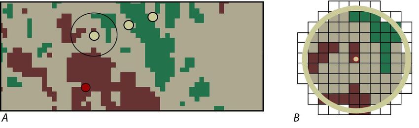
Table 6–1. Area, sediment-thickness, and sediment-volume data for California’s State Waters in Santa Barbara
           Channel region, between Point Conception and Hueneme Canyon areas, as well as in the Offshore of
           Gaviota map area. ................................................................................................................................. 24
Table 7–1. Areas and relative proportions of offshore geologic map units in Offshore of Gaviota map area .......... 28

Map Sheets
Sheet 1.         Colored Shaded-Relief Bathymetry, Offshore of Gaviota Map Area, California
                   By Peter Dartnell and Rikk G. Kvitek
Sheet 2.         Shaded-Relief Bathymetry, Offshore of Gaviota Map Area, California
                   By Peter Dartnell and Rikk G. Kvitek
Sheet 3.         Acoustic Backscatter, Offshore of Gaviota Map Area, California
                   By Peter Dartnell and Rikk G. Kvitek
Sheet 4.         Data Integration and Visualization, Offshore of Gaviota Map Area, California
                   By Peter Dartnell
Sheet 5.         Seafloor Character, Offshore of Gaviota Map Area, California
                   By Stephen R. Hartwell and Guy R. Cochrane
Sheet 6.         Marine Benthic Habitats from the Coastal and Marine Ecological Classification Standard, Offshore of
                 Gaviota Map Area, California
                   By Guy R. Cochrane, Stephen R. Hartwell, and Samuel Y. Johnson
Sheet 7.         Seismic-Reflection Profiles, Offshore of Gaviota Map Area, California
                   By Samuel Y. Johnson and Stephen R. Hartwell
Sheet 8.         Local (Offshore of Gaviota Map Area) and Regional (Offshore from Point Conception to Hueneme
                 Canyon) Shallow-Subsurface Geology and Structure, Santa Barbara Channel, California
                   By Samuel Y. Johnson and Stephen R. Hartwell
Sheet 9.         Offshore and Onshore Geology and Geomorphology, Offshore of Gaviota Map Area, California
                   By Stephen R. Hartwell, Samuel Y. Johnson, and Clifton W. Davenport

                                                                               iv
California State Waters Map Series—Offshore of Gaviota,
California
By Samuel Y. Johnson,1 Peter Dartnell,1 Guy R. Cochrane,1 Stephen R. Hartwell,1 Nadine E. Golden,1 Rikk G.
Kvitek,2 and Clifton W. Davenport3
(Samuel Y. Johnson1 and Susan A. Cochran,1 editors)
Preface
In 2007, the California Ocean Protection Council initiated the California Seafloor Mapping
Program (CSMP), designed to create a comprehensive seafloor map of high-resolution bathymetry,
marine benthic habitats, and geology within California’s State Waters. The program supports a large
number of coastal-zone- and ocean-management issues, including the California Marine Life Protection
Act (MLPA) (California Department of Fish and Wildlife, 2008), which requires information about the
distribution of ecosystems as part of the design and proposal process for the establishment of Marine
Protected Areas. A focus of CSMP is to map California’s State Waters with consistent methods at a
consistent scale.
The CSMP approach is to create highly detailed seafloor maps through collection, integration,
interpretation, and visualization of swath sonar bathymetric data (the undersea equivalent of satellite
remote-sensing data in terrestrial mapping), acoustic backscatter, seafloor video, seafloor photography,
high-resolution seismic-reflection profiles, and bottom-sediment sampling data (Johnson and others,
2017). The map products display seafloor morphology and character, identify potential marine benthic
habitats, and illustrate both the surficial seafloor geology and shallow subsurface geology. It is
emphasized that the more interpretive habitat and geology maps rely on the integration of multiple, new
high-resolution datasets and that mapping at small scales would not be possible without such data.
This approach and CSMP planning is based in part on recommendations of the Marine Mapping
Planning Workshop (Kvitek and others, 2006), attended by coastal and marine managers and scientists
from around the state. That workshop established geographic priorities for a coastal mapping project and
identified the need for coverage of “lands” from the shore strand line (defined as Mean Higher High
Water; MHHW) out to the 3-nautical-mile (5.6-km) limit of California’s State Waters. Unfortunately,
surveying the zone from MHHW out to 10-m water depth is not consistently possible using ship-based
surveying methods, owing to sea state (for example, waves, wind, or currents), kelp coverage, and
shallow rock outcrops. Accordingly, some of the maps presented in this series commonly do not cover
the zone from the shore out to 10-m depth; these “no data” zones appear pale gray on most maps.
This map is part of a series of online U.S. Geological Survey (USGS) publications, each of
which includes several map sheets, some explanatory text, and a descriptive pamphlet. Each map sheet
is published as a PDF file. Geographic information system (GIS) files that contain both ESRI4 ArcGIS
raster grids (for example, bathymetry, seafloor character) and geotiffs (for example, shaded relief) are
also included for each publication. For those who do not own the full suite of ESRI GIS and mapping
software, the data can be read using ESRI ArcReader, a free viewer that is available at
1
U.S. Geological Survey
2
California State University, Monterey Bay, Seafloor Mapping Lab
3
California Geological Survey
4
Environmental Systems Research Institute, Inc.
1http://www.esri.com/software/arcgis/arcreader/index.html (last accessed March 27, 2016). Web services,
which consist of standard implementations of ArcGIS REST Service and OGC GIS Web Service
(WMS), also are available for all published GIS data. All CSMP web services were created using an
ArcGIS service definition file, resulting in data layers that are symbolized as shown on the associated
map sheets. Both the ArcGIS REST Service and OGC WMS Service include all the individual GIS
layers for each map-area publication. Data layers are bundled together in a map-area web service;
however, each layer can be symbolized and accessed individually after the web service is ingested into a
desktop application or web map. CSMP web services enable users to download and view CSMP data, as
well as to easily add CSMP data to their own workflows, using any browser-enabled, standalone or
mobile device.
The California Seafloor Mapping Program (CSMP) is a collaborative venture between numerous
different federal and state agencies, academia, and the private sector. CSMP partners include the
California Coastal Conservancy, the California Ocean Protection Council, the California Department of
Fish and Wildlife, the California Geological Survey, California State University at Monterey Bay’s
Seafloor Mapping Lab, Moss Landing Marine Laboratories Center for Habitat Studies, Fugro Pelagos,
Pacific Gas and Electric Company, National Oceanic and Atmospheric Administration (NOAA,
including National Ocean Service—Office of Coast Surveys, National Marine Sanctuaries, and National
Marine Fisheries Service), U.S. Army Corps of Engineers, the Bureau of Ocean Energy Management,
the National Park Service, and the U.S. Geological Survey.
2Chapter 1. Introduction
By Samuel Y. Johnson
Regional Setting
The map area offshore of Gaviota, California, which is referred to herein as the “Offshore of
Gaviota” map area (figs. 1–1, 1–2), lies within the western Santa Barbara Channel region of the
Southern California Bight (see, for example, Lee and Normark, 2009). This geologically complex region
forms a major biogeographic transition zone, separating the cold-temperate Oregonian province north of
Point Conception from the warm-temperate California province to the south (Briggs, 1974). Within this
region, the offshore part of the map area lies south of the steep south flank of the Santa Ynez Mountains.
The crest of the range, which lies about 4 km north of the shoreline, has a maximum elevation of about
760 m.
Gaviota (Spanish for “seagull”) is an unincorporated community that has a sparse population
(less than 100), and the coastal zone is largely open space that is locally used for cattle grazing. The
Union Pacific railroad tracks extend westward along the coast through the entire map area, within a few
hundred meters of the shoreline. Highway 101 crosses the eastern part of the map area, also along the
coast, then turns north (inland) and travels through Cañada de la Gaviota and Gaviota Pass en route to
Buellton (fig. 1–1). Gaviota State Park lies at the mouth of Cañada de la Gaviota (fig. 1–2). West of
Gaviota, the onland coastal zone is occupied by the Hollister Ranch, a privately owned, gated
community that has no public access.
The map area has a long history of petroleum exploration and development. Several offshore gas
fields were discovered and were developed by onshore directional drilling in the 1950s and 1960s
(Yerkes and others, 1969; Galloway, 1998). Three offshore petroleum platforms were installed in
adjacent federal waters in 1976 (platform “Honda”) and 1989 (platforms “Heritage” and “Harmony”).
Local offshore and onshore operations were serviced for more than a century by the Gaviota marine
terminal (fig. 1–2), a site that has been variably used for more than a century as an asphalt refinery, oil
refinery, crude-oil marine terminal, crude-oil-pipeline terminal, and other operations (County of Santa
Barbara, Planning and Development, Energy Division, 2016). The marine terminal is currently being
decommissioned and will be abandoned in an intended transition to public open space.
The Offshore of Gaviota map area lies in the western-central part of the Santa Barbara littoral
cell (fig. 1–1), which is characterized by west-to-east transport of sediment from Point Arguello on the
northwest to Hueneme and Mugu Canyons on the southeast (see, for example, Griggs and others, 2005;
Hapke and others, 2006). Sediment supply to the western and central part of the littoral cell is mainly
from relatively small coastal watersheds, which have an estimated cumulative annual sediment flux of
640,000 tons/yr between Point Arguello and the Ventura River (fig. 1–1; see also, Warrick and
Farnsworth, 2009). Consistent with this estimate, Griggs and others (2005) reported dredging records
from the harbor at Santa Barbara that range from about 160,000 to 800,000 tons/yr, averaging 400,000
tons/yr, providing a proxy for longshore drift rates.
Cañada de la Gaviota is the largest coastal watershed (about 52 km2; Warrick and Mertes, 2009)
between the Ventura River and Point Conception, and it is inferred to be the largest sediment source in
this zone. Smaller watersheds in the Offshore of Gaviota map area include Cañada de la Llegua, Arroyo
el Bulito, Cañada de Santa Anita, Cañada de Alegria, Cañada del Agua Caliente, Cañada del Barro,
Cañada del Leon, Cañada San Onofre, and many others (fig. 1–2). The much larger Santa Ynez and
Santa Maria Rivers, the mouths of which are 60 to 100 km northwest of the map area (following the
coast; fig. 1–1), are not considered to be significant sediment sources because Point Conception and
Point Arguello (fig. 1–1) provide obstacles to downcoast, southeastward sediment transport and also
because, at present, much of their sediment load is trapped in dams (Griggs and others, 2005).
3Coastal-watershed discharge and sediment load are highly variable, characterized by brief large
events during major winter storms and long periods of low (or no) flow and minimal sediment load
between storms. In recent (recorded) history, the majority of high-discharge, high-sediment-flux events
have been associated with El Niño phases of the El Niño–Southern Oscillation (ENSO) climatic pattern
(Warrick and Farnsworth, 2009).
Narrow beaches that have thin sediment (sand and pebbles) cover, backed by low (10- to 20-m-
high) cliffs that are capped by a narrow coastal terrace, characterize the shoreline in the Offshore of
Gaviota map area. Beaches are subject to wave erosion during winter storms, followed by gradual
sediment recovery or accretion in the late spring, summer, and fall months during the gentler wave
climate. Hapke and others (2006, their fig. 33) suggested that essentially no net change (accretion or
erosion) to the beaches in the map area has occurred in the long term (since the mid- to late-1800s);
however, the beaches have been eroding at an average rate of about 0.6 m/yr in the short term (1976 to
1998). Hapke and Reid (2007, their fig. 29) also indicated that coastal bluffs in the map area are eroding
at a rate of about 0.2 m/yr. As with stream discharge and sediment flux, coastal erosion has been most
acute during El Niño phases of the ENSO climatic pattern.
The offshore Gaviota sediment bar (fig. 1–2), which extends southwestward for about 9 km from
the mouth of Cañada de la Gaviota to the shelf break, is as wide as 2 km, and it is by far the largest
shore-attached sediment bar in the Santa Barbara Channel. The bar, which faces southeast, has a
relatively flat (~1.4°) top that extends to water depths of 60 m. The front of the bar has failed
intermittently, and the steep (as much as 5°) bar front is bounded by an apron of coalescing mass-flow
lobes.
Shelf width in the Offshore of Gaviota map area ranges from about 4.3 to 4.7 km, and shelf
slopes average about 1.0° to 1.2° but are highly variable because of the presence of the large Gaviota
sediment bar. The shelf is underlain by bedrock and variable amounts (0 to as much as 36 m in the
Gaviota bar) of upper Quaternary sediments deposited as sea level fluctuated in the late Pleistocene (see
sheet 9 of this report; see also, Slater and others, 2002; Draut and others, 2009; Sommerfield and others,
2009).
This part of the Southern California Bight is somewhat protected from large Pacific swells from
the north and northwest by Point Conception and from south and southwest swells by offshore islands
and banks (O’Reilly and Guza, 1993; Cudaback and others, 2005). Fair-weather wave base is typically
shallower than 20-m water depth, but winter storms are capable of resuspending fine-grained sediments
in 30 m of water (Xu and Noble, 2009, their table 7), and so shallow (depths of 30 to 60 m) shelf
sediments in the map area probably are remobilized on an annual basis. As with sediment discharge
from rivers, the largest wave events and the highest sediment-transport rates on the shelf are typically
associated with the El Niño phases of the ENSO climatic pattern (Xu and Noble, 2009).
Within the map area, the trend of the shelf break changes from about 276° to 236° azimuth over
a distance of about 12 km, and it ranges in depth from about 91 m to as shallow as 62 to 73 m where
significant shelf-break and upper-slope failure and landsliding has apparently occurred. Below the shelf
break in the eastern part of the map area, the upper slope is relatively smooth, and slopes it offshore as
much as 6°. The shelf break in the western part of the map area is notably embayed by the heads of three
large (150- to 300-m-wide) channels that have been referred to as “the Gaviota Canyons” (Fischer and
Cherven, 1998) or as “Drake Canyon,” “Sacate Canyon,” and “Alegria Canyon” (Eichhubl and others,
2002).
Seafloor habitats in the broad Santa Barbara Channel region consist of significant amounts of
soft, unconsolidated sediment interspersed with isolated areas of rocky habitat that support kelp-forest
communities in the nearshore and rocky-reef communities in deeper water. The potential marine benthic
habitat types mapped in the Offshore of Gaviota map area are directly related to its Quaternary geologic
history, geomorphology, and active sedimentary processes. These potential habitats lie primarily within
4the Shelf (continental shelf) but also partly within the Flank (basin flank or continental slope)
megahabitats of Greene and others (2007). The fairly homogeneous seafloor of sediment and low-relief
bedrock provides characteristic habitat for groundfish, crabs, shrimp, and other marine benthic
organisms, and the bedrock outcrops are potential benthic habitats for rockfish (Sebastes spp.) and other
groundfish that forage and seek refuge in such habitats. In addition, several areas of smooth sediment
that form nearshore terraces that have relatively steep, smooth fronts may provide interfaces attractive to
certain species of groundfish. Below the steep shelf break, within the basin flank or continental slope
megahabitat, the seafloor is composed of soft, unconsolidated sediment interrupted by the heads of
several submarine canyons and rills, some bedrock exposures, and small carbonate mounds associated
with asphalt mounds and pockmarks. The steep shelf break and carbonate mounds are also good
potential habitat for rockfish. The map area includes the relatively small (5.2 km2) Kashtayit State
Marine Conservation Area (fig. 1–2), which largely occupies the inner part of the Gaviota sediment bar.
The Offshore of Gaviota map area is in the southern part of the Western Transverse Ranges
geologic province, which is north of the California Continental Borderland5 (Fisher and others, 2009).
Significant clockwise rotation—at least 90°—since the early Miocene has been proposed for the
Western Transverse Ranges province (Luyendyk and others, 1980; Hornafius and others, 1986;
Nicholson and others, 1994), and this region is presently undergoing north-south shortening (see, for
example, Larson and Webb, 1992; Marshall and others, 2013). Regional cross sections (Tennyson and
Kropp, 1998; Redin and others, 2005) have suggested that the south flank of the Santa Ynez Mountains
is a large, south-dipping homocline that overlies the north-dipping Pitas Point–North Channel Fault
system (fig. 1–3; see also, Sorlien and Nicholson, 2015). The homoclinal section extends upward from
the Cretaceous strata exposed high in the mountains to the Pliocene strata beneath the continental shelf,
encountered at shallow depths in offshore wells. Smaller folds (see sheets 7, 8, 9) related to local
faulting are superimposed on the regional homocline, including the 17-km-long Molino Anticline and
the 22-km-long Government Point Syncline (see sheets 8, 9).
Coastal cliffs mainly consist of fine-grained, folded strata of the Miocene Monterey Formation
and the upper Miocene and lower Pliocene Sisquoc Formation (Dibblee, 1988a,b). Estimated rates of
shoreline uplift that are based on the elevations of late Quaternary marine terraces are highly variable,
ranging from about 0.25 to 1.8 mm/yr (Muhs and others, 1992; Rockwell and others, 1992; Metcalf,
1994; Duvall and others, 2004; Gurrola and others, 2014).
Publication Summary
This publication about the Offshore of Gaviota map area includes nine map sheets that contain
explanatory text, in addition to this descriptive pamphlet and a data catalog of geographic information
system (GIS) files. Sheets 1, 2, and 3 combine data from three different sonar surveys to generate
comprehensive high-resolution bathymetry and acoustic-backscatter coverage of the map area. These
data reveal a range of physiographic features (highlighted in the perspective views on sheet 4) such as
the flat, sediment-covered Santa Barbara shelf interspersed with tectonically controlled bedrock uplifts
and coarse-grained deltas and sediment lobes associated with coastal watersheds. To validate the
geological and biological interpretations of the sonar data shown on sheets 1, 2, and 3, the U.S.
Geological Survey towed a camera sled over specific offshore locations, collecting both video and
photographic imagery; this “ground-truth” surveying imagery is available at Golden and Cochrane
(2013). Sheet 5 is a “seafloor character” map, which classifies the seafloor on the basis of depth, slope,
rugosity (ruggedness), and backscatter intensity and which is further informed by the ground-truth-
survey imagery. Sheet 6 is a map of “potential habitats,” which are delineated on the basis of substrate
5
The California Continental Borderland is defined as the complex continental margin that extends from Point Conception
south into northern Baja California.
5type, geomorphology, seafloor process, or other attributes that may provide a habitat for a specific
species or assemblage of organisms. Sheet 7 compiles representative seismic-reflection profiles from the
map area, providing information on the subsurface stratigraphy and structure of the map area. Sheet 8
shows the distribution and thickness of young sediment (deposited over the last about 21,000 years,
during the most recent sea-level rise) in both the map area and the larger Santa Barbara Channel region
(offshore from Point Conception to Hueneme Canyon), interpreted on the basis of the seismic-reflection
data. Sheet 9 is a geologic map that merges onshore geologic mapping (compiled from existing maps by
the California Geological Survey) and new offshore geologic mapping that is based on integration of
high-resolution bathymetry and backscatter imagery (sheets 1, 2, 3), seafloor-sediment and rock samples
(Reid and others, 2006), digital camera and video imagery (Golden and Cochrane, 2013), and high-
resolution seismic-reflection profiles (sheet 7).
The information provided by the map sheets, pamphlet, and data catalog have a broad range of
applications (Johnson and others, 2017). High-resolution bathymetry, acoustic backscatter, ground-truth-
surveying imagery, and habitat mapping all contribute to habitat characterization and ecosystem-based
management by providing essential data for delineation of marine protected areas and ecosystem
restoration. Many of the maps provide high-resolution baselines that will be critical for monitoring
environmental change associated with climate change, coastal development, or other forcings. High-
resolution bathymetry is a critical component for modeling coastal flooding caused by storms and
tsunamis, as well as inundation associated with longer term sea-level rise. Seismic-reflection and
bathymetric data help characterize earthquake and tsunami sources, critical for natural-hazard
assessments of coastal zones. Information on sediment distribution and thickness is essential to the
understanding of local and regional sediment transport, as well as the development of regional sediment-
management plans. In addition, siting of any new offshore infrastructure (for example, pipelines, cables,
or renewable-energy facilities) will depend on new high-resolution mapping. Finally, this mapping will
both stimulate and enable new scientific research and also raise public awareness of, and education
about, coastal environments and issues.
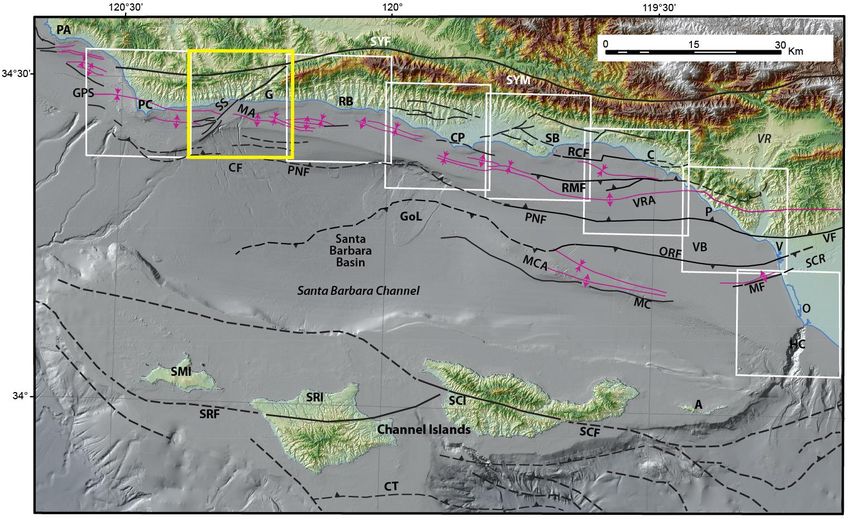
6Figure 1–1. Physiography of Santa Barbara Channel region. Box shows Offshore of Gaviota map area. Arrows
show direction of sediment transport in Santa Barbara littoral cell, which extends from Point Arguello (PA) to
Hueneme Canyon (HC) and Mugu Canyon (MC). Other abbreviations: B, Buellton; C, Carpinteria; CC,
Calleguas Creek; G, Goleta; GoL, Goleta landslide complex; O, Oxnard; PC, Point Conception; SB, Santa
Barbara; SBB, Santa Barbara Basin; SM, Santa Monica Mountains; SMB, Santa Monica Basin; SMR, Santa
Maria River; SR, Santa Clara River; SYM, Santa Ynez Mountains; SYR, Santa Ynez River; V, Ventura; VR,
Ventura River.
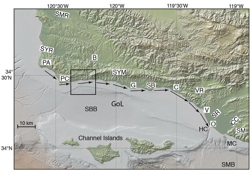
7Figure 1–2. Coastal geography of Offshore of Gaviota map area. Yellow line shows 3-nautical-mile limit of
California’s State Waters. Blue line shows boundary of Kashtayit State Marine Conservation Area (KSM). Other
abbreviations: AB, Arroyo el Bulito; AC, “Alegria Canyon;” CA, Cañada de Alegria; CAC, Cañada del Agua
Caliente; CB, Cañada del Barro; CG, Cañada de la Gaviota; CL, Cañada del Leon; CLL, Cañada de la Llegua;
CS, Cañada San Onofre; CSA, Cañada de Santa Anita; DC, “Drake Canyon;” G, Gaviota; GB, Gaviota
sediment bar; GM, Gaviota marine terminal; GP, Gaviota Pass; GSP, Gaviota State Park; SC, “Sacate
Canyon.”
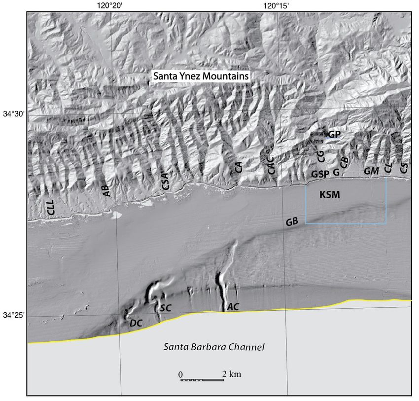
8Figure 1–3. Map of Santa Barbara Channel region, showing selected faults and folds. Black lines show faults (solid
where location is known; dashed where location is approximate or inferred); barbs on faults show thrust faults
(barbs on upper plate); locations of blind Pitas Point–North Channel Fault (PNF) and Oak Ridge Thrust Fault
(ORF) systems are projected vertically from tips of faults. Magenta lines show folds (solid where location is
known; diverging arrows show anticlines; converging arrows show synclines. Yellow box shows outline of
Offshore of Gaviota map area. White boxes show outlines of maps and datasets published by U.S. Geological
Survey’s California Seafloor Mapping Program (CSMP), listed from east to west (map area names shown in
brackets): Johnson and others, 2012 [Hueneme Canyon], 2013b [Ventura], 2013c [Carpinteria], 2013a [Santa
Barbara], 2014 [Coal Oil Point], 2015 [Refugio Beach], 2018 [Point Conception]. Fault locations are from Sorlien
and others (2006), Chaytor and others (2008), Minor and others (2009), and U.S. Geological Survey and
California Geological Survey (2016), as well as from CSMP publications listed above. Other abbreviations: A,
Anacapa Island; C, Carpinteria; CF, Conception fan; CP, Coal Oil Point; CT, Channel Islands Thrust Fault; G,
Gaviota; GoL, Goleta landslide complex; GPS, Government Point Syncline; HC, Hueneme Canyon; MA, Molino
Anticline; MC, Mid-Channel Fault; MCA, Mid-Channel Anticline; MF, Montalvo Fault; O, Oxnard; P, Pitas Point;
PA, Point Arguello; PC, Point Conception; RB, Refugio Beach; RCF, Rincon Creek Fault; RMF, Red Mountain
Fault; SB, Santa Barbara; SCF, Santa Cruz Island Fault; SCI, Santa Cruz Island; SCR, Santa Clara River; SMI,
San Miguel Island; SRF, Santa Rosa Island Fault; SRI, Santa Rosa Island; SS, south strand of Santa Ynez
Fault; SYF, Santa Ynez Fault; SYM, Santa Ynez Mountains; V, Ventura; VB, Ventura Basin; VF, Ventura Fault;
VR, Ventura River; VRA, Ventura Avenue–Rincon–South Ellwood Anticline.
9Chapter 2. Bathymetry and Backscatter-Intensity Maps of the Offshore
of Gaviota Map Area (Sheets 1, 2, and 3)
By Peter Dartnell and Rikk G. Kvitek
The colored shaded-relief bathymetry (sheet 1), the shaded-relief bathymetry (sheet 2), and the
acoustic-backscatter (sheet 3) maps of the Offshore of Gaviota map area in southern California were
generated from bathymetry and backscatter data collected by the U.S. Geological Survey (USGS) and by
Fugro Pelagos (fig. 1 on sheets 1, 2, 3) in 2007 and 2008, using a combination of 400-kHz Reson 7125,
240-kHz Reson 8101, and 100-kHz Reson 8111 multibeam echosounders, as well as a 234-kHz SEA
SWATHplus bathymetric sidescan-sonar system. In addition, bathymetric- and topographic-lidar data
was collected in the nearshore and coastal areas by the U.S. Army Corps of Engineers (USACE) Joint
Lidar Bathymetry Technical Center of Expertise in 2009 and 2010. These mapping missions combined
to provide continuous bathymetry (sheets 1, 2) from the shoreline to the 3-nautical-mile limit of
California’s State Waters, as well as acoustic-backscatter data (sheet 3) from about the 10-m isobath to
beyond the 3-nautical-mile limit.
During the USGS mapping missions, GPS data with real-time-kinematic corrections were
combined with measurements of vessel motion (heave, pitch, and roll) in a CodaOctopus F190 attitude-
and-position system to produce a high-precision vessel-attitude packet. This packet was transmitted to
the acquisition software in real time and combined with instantaneous sound-velocity measurements at
the transducer head before each ping. The returned samples were projected to the seafloor using a ray-
tracing algorithm that works with previously measured sound-velocity profiles. Statistical filters were
applied to discriminate seafloor returns (soundings and backscatter intensity) from unintended targets in
the water column. Further editing of the USGS 2007 bathymetric-sounding data was completed in 2016,
and the final soundings were converted into a 2-m-resolution bathymetric-surface-model grid. The
backscatter data were postprocessed (also in 2016) using SonarWiz software that normalizes for time-
varying signal loss and beam-directivity differences. Thus, the raw 16-bit backscatter data were gain-
normalized to enhance the backscatter of the SWATHplus system. The data were exported in Imagine
format, imported into a geographic information system (GIS), and converted to a GRID at 2-m
resolution.
During the Fugro Pelagos mapping missions, an Applanix POS-MV (Position and Orientation
System for Marine Vessels) was used to accurately position the vessels during data collection, and it
also accounted for vessel motion such as heave, pitch, and roll, with navigational input from GPS
receivers. Smoothed Best Estimated Trajectory (SBET) files were postprocessed from logged POS-MV
files. Sound-velocity profiles were collected with an Applied Microsystems (AM) SVPlus sound
velocimeter. Soundings were corrected for vessel motion using the Applanix POS-MV data, for
variations in water-column sound velocity using the AM SVPlus data, and for variations in water height
(tides) and heave using the postprocessed SBET data (California State University, Monterey Bay,
Seafloor Mapping Lab, 2016). The Reson backscatter data were postprocessed using Geocoder software.
The backscatter intensities were radiometrically corrected (including despeckling and angle-varying gain
adjustments), and the position of each acoustic sample was geometrically corrected for slant range on a
line-by-line basis. After the lines were corrected, they were mosaicked into 0.5-m resolution images
(California State University, Monterey Bay, Seafloor Mapping Lab, 2016). The mosaics were then
exported as georeferenced TIFF images, imported into a GIS, and converted to GRIDs at 2-m resolution.
Nearshore bathymetric-lidar data and acoustic-bathymetric data from within California’s State
Waters were merged together as part of the 2013 National Oceanic and Atmospheric Administration
(NOAA) Coastal California TopoBathy Merge Project (National Oceanic and Atmospheric
Administration, 2013). Merged bathymetry data from within the Offshore of Gaviota map area were
10downloaded from this dataset and resampled to 2-m spatial resolution, then the reprocessed 2007 USGS
bathymetry data was incorporated into the downloaded data. An illumination having an azimuth of 300°
and from 45° above the horizon was then applied to the new bathymetric surface to create the shaded-
relief imagery (sheets 1, 2). In addition, a “rainbow” color ramp was applied to the bathymetry data for
sheet 1, using reds to represent shallower depths, and blueish greens (and in deeper submarine canyons,
purples) to represent greater depths. This colored bathymetry surface was draped over the shaded-relief
imagery at 60-percent transparency to create a colored shaded-relief map (sheet 1). Note that the ripple
patterns and parallel lines that are apparent within the map area are data-collection and -processing
artifacts. These various artifacts are made obvious by the hillshading process.
Bathymetric contours (sheets 1, 2, 3, 5, 6, 9) were generated at 10-m intervals from a modified 2-
m-resolution bathymetric surface. The most continuous contour segments were preserved; smaller
segments and isolated island polygons were excluded from the final output. The contours were
smoothed using a polynomial approximation with exponential kernel algorithm and a tolerance value of
60 m. The contours were then clipped to the boundary of the map area.
The acoustic-backscatter imagery from each different mapping system and processing method
were merged into their own individual grids. These individual grids, which cover different areas, were
displayed in a GIS to create a composite acoustic-backscatter map (sheet 3). On the map, brighter tones
indicate higher backscatter intensity, and darker tones indicate lower backscatter intensity. The intensity
represents a complex interaction between the acoustic pulse and the seafloor, as well as characteristics
within the shallow subsurface, providing a general indication of seafloor texture and composition.
Backscatter intensity depends on the acoustic source level; the frequency used to image the seafloor; the
grazing angle; the composition and character of the seafloor, including grain size, water content, bulk
density, and seafloor roughness; and some biological cover. Harder and rougher bottom types such as
rocky outcrops or coarse sediment typically return stronger intensities (high backscatter, lighter tones),
whereas softer bottom types such as fine sediment return weaker intensities (low backscatter, darker
tones). Ripple patterns and straight lines in some parts of the map area are data-collection and
-processing artifacts.
The onshore-area image was generated by applying an illumination having an azimuth of 300°
and from 45° above the horizon to 2-m-resolution topographic-lidar data from National Oceanic and
Atmospheric Administration Office for Coastal Management’s Digital Coast (available at
http://www.csc.noaa.gov/digitalcoast/data/coastallidar/) and to 10-m-resolution topographic-lidar data
from the U.S. Geological Survey’s National Elevation Dataset (available at http://ned.usgs.gov/).
11Chapter 3. Data Integration and Visualization for the Offshore of
Gaviota Map Area (Sheet 4)
By Peter Dartnell
Mapping California’s State Waters has produced a vast amount of acoustic and visual data,
including bathymetry, acoustic backscatter, seismic-reflection profiles, and seafloor video and
photography. These data are used by researchers to develop maps, reports, and other tools to assist in the
coastal and marine spatial-planning capability of coastal-zone managers and other stakeholders. For
example, seafloor-character (sheet 5), habitat (sheet 6), and geologic (sheet 9) maps of the Offshore of
Gaviota map area may be used to assist in the designation of Marine Protected Areas, as well as in their
monitoring. These maps and reports also help to analyze environmental change owing to sea-level rise
and coastal development, to model and predict sediment and contaminant budgets and transport, to site
offshore infrastructure, and to assess tsunami and earthquake hazards. To facilitate this increased
understanding and to assist in product development, it is helpful to integrate the different datasets and
then view the results in three-dimensional representations such as those displayed on the data integration
and visualization sheet for the Offshore of Gaviota map area (sheet 4).
The maps and three-dimensional views on sheet 4 were created using a series of geographic
information systems (GIS) and visualization techniques. Using GIS, the bathymetric and topographic
data (sheet 1) were converted to ASCIIRASTER format files, and the acoustic-backscatter data (sheet 3)
were converted to geoTIFF images. The bathymetric and topographic data were imported in the
Fledermaus software (QPS). The bathymetry was color-coded to closely match the colored shaded-
relief bathymetry on sheet 1 in which reds and oranges represent shallower depths and blueish greens
(and purples, in submarine canyons) represent deeper depths. Onshore topographic data were shown in
gray shades. Acoustic-backscatter geoTIFF images also were draped over the bathymetry data (fig. 6).
The colored bathymetry, topography, and draped backscatter were then tilted and panned to create the
perspective views such as those shown in figures 1, 2, 4, 5, and 6 on sheet 4. These views highlight the
seafloor morphology in the Offshore of Gaviota map area, which includes asphalt mounds, rock outcrops,
gullies, sediment mass-flow deposits, and linear striations interpreted as trawling scars.
Video-mosaic images created from digital seafloor video (for example, fig. 3 on sheet 4) can
display the geologic complexity (rock, sand, and mud; see sheet 9) and biologic complexity (see Golden
and Cochrane, 2013) of the seafloor. Whereas photographs capture high-quality snapshots of smaller
areas of the seafloor, video mosaics capture larger areas and can show transition zones between seafloor
environments. Digital seafloor video is collected from a camera sled towed approximately 1 to 2 meters
above the seafloor, at speeds of less than 1 nautical mile/hour. Using standard video-editing software, as
well as software developed at the Center for Coastal and Ocean Mapping, University of New
Hampshire, the digital video is converted to AVI format, cut into 2-minute sections, and desampled to
every second or third frame. The frames are merged together using pattern-recognition algorithms from
one frame to the next and converted to a TIFF image. The images are then rectified to the bathymetry
data using ship navigation recorded with the video and layback estimates of the towed camera sled.
Block diagrams that combine the bathymetry with seismic-reflection-profile data help integrate
surface and subsurface observations, especially stratigraphic and structural relations (for example, fig. 1
on sheet 4). These block diagrams were created by converting digital seismic-reflection-profile data
(Johnson and others, 2016) into TIFF images, while taking note of the starting and ending coordinates
and maximum and minimum depths. The images were then imported into the Fledermaus software as
vertical images and merged with the bathymetry imagery.
12Chapter 4. Seafloor-Character Map of the Offshore of Gaviota Map Area
(Sheet 5)
By Guy R. Cochrane and Stephen R. Hartwell
The California State Marine Life Protection Act (MLPA) calls for protecting representative types
of habitat in different depth zones and environmental conditions. A science team, assembled under the
auspices of the California Department of Fish and Wildlife (CDFW), has identified seven substrate-
defined seafloor habitats in California’s State Waters that can be classified using sonar data and seafloor
video and photography. These habitats include rocky banks, intertidal zones, sandy or soft ocean
bottoms, underwater pinnacles, kelp forests, submarine canyons, and seagrass beds. The following five
depth zones, which determine changes in species composition, have been identified: Depth Zone 1,
intertidal; Depth Zone 2, intertidal to 30 m; Depth Zone 3, 30 to 100 m; Depth Zone 4, 100 to 200 m;
and Depth Zone 5, deeper than 200 m (California Department of Fish and Wildlife, 2008). The CDFW
habitats, with the exception of depth zones, can be considered a subset of a broader classification
scheme of Greene and others (1999) that has been used by the U.S. Geological Survey (USGS)
(Cochrane and others, 2003, 2005). These seafloor-character maps are generalized polygon shapefiles
that have attributes derived from Greene and others (2007).
A 2007 Coastal Map Development Workshop, hosted by the USGS in Menlo Park, California,
identified the need for more detailed (relative to Greene and others’ [1999] attributes) raster products
that preserve some of the transitional character of the seafloor when substrates are mixed and (or) they
change gradationally. The seafloor-character map, which delineates a subset of the CDFW habitats, is a
GIS-derived raster product that can be produced in a consistent manner from data of variable quality
covering large geographic regions.
The following five substrate classes are identified in the Offshore of Gaviota map area:
Class I: Fine- to medium-grained smooth sediment
Class II: Mixed smooth sediment and rock
Class III: Rock and boulder, rugose
Class IV: Medium- to coarse-grained sediment (in scour depressions)
Class V: Anthropogenic material (rugged)
The seafloor-character map of the Offshore of Gaviota map area (sheet 5) was produced using
video-supervised maximum-likelihood classification of the bathymetry and intensity of return from
sonar systems, following the method described by Cochrane (2008). The two variants used in this
classification were backscatter intensity and derivative rugosity. The rugosity calculation was performed
using the Terrain Ruggedness (VRM) tool within the Benthic Terrain Modeler toolset v. 3.0 (Wright and
others, 2012; available at http://esriurl.com/5754).
Classes I, II, and III values were delineated using multivariate analysis. Class IV (medium- to
coarse-grained sediment, in scour depressions) values were determined on the basis of their visual
characteristics, using both shaded-relief bathymetry and backscatter (slight depression in the seafloor,
very high backscatter return). Class V (rugged anthropogenic material) values were determined on the
basis of their visual characteristics and the known location of man-made features. The resulting map
(gridded at 2 m) was cleaned by hand to remove data-collection artifacts (for example, the trackline
nadir).
On the seafloor-character map (sheet 5), the five substrate classes have been colored to indicate
the California MLPA depth zones and the Coastal and Marine Ecological Classification Standard
(CMECS) slope zones (Madden and others, 2008) in which they belong. The California MLPA depth
13zones are Depth Zone 1 (intertidal), Depth Zone 2 (intertidal to 30 m), Depth Zone 3 (30 to 100 m),
Depth Zone 4 (100 to 200 m), and Depth Zone 5 (greater than 200 m); in the Offshore of Gaviota map
area, only Depth Zones 2, 3, and 4 are present. The slope classes that represent the CMECS slope zones
are Slope Class 1 = flat (0° to 5°), Slope Class 2 = sloping (5° to 30°), Slope Class 3 = steeply sloping
(30° to 60°), Slope Class 4 = vertical (60° to 90°), and Slope Class 5 = overhang (greater than 90°); in
the Offshore of Gaviota map area, only Slope Classes 1, 2, and 3 are present. The final classified
seafloor-character raster map image has been draped over the shaded-relief bathymetry for the area
(sheets 1 and 2) to produce the image shown on the seafloor-character map on sheet 5.
The seafloor-character classification also is summarized on sheet 5 in table 1. Fine- to medium-
grained smooth sediment (sand and mud) makes up 78.8 percent (75.1 km2) of the map area: 21.6
percent (20.6 km2) is in Depth Zone 2, 46.7 percent (44.5 km2) is in Depth Zone 3, and 10.5 percent
(10.0 km2) is in Depth Zone 4. Mixed smooth sediment (sand and gravel) and rock (that is, sediment
typically forming a veneer over bedrock, or rock outcrops having little to no relief) make up 16.2
percent (15.4 km2) of the map area: 6.1 percent (5.9 km2) is in Depth Zone 2, 8.0 percent (7.7 km2) is in
Depth Zone 3, and 2.0 percent (1.9 km2) is in Depth Zone 4. Rock and boulder, rugose (rock outcrops,
boulder fields, and asphalt mounds having high surficial complexity) makes up 4.9 percent (4.7 km2) of
the map area: 2.0 percent (1.9 km2) is in Depth Zone 2, 1.7 percent (1.7 km2) is in Depth Zone 3, and 1.3
percent (1.2 km2) is in Depth Zone 4. Medium- to coarse-grained sediment (in scour depressions
consisting of material that is coarser than the surrounding seafloor), which makes up less than 0.1
percent (in Cochrane, 2008) and the limited ground-truth information available when compared to the continuous
coverage provided by swath sonar. Presence/absence values in table 4–2 reflect the percentages of
observations where the sediment classification of at least one pixel within the buffer zone agreed with
the observed sediment type at a certain location.
The classification accuracies are shown in table 4–2. The weaker agreements in Class II (53.7
percent accurate) and Class III (42.9 percent accurate) likely are due to the relatively narrow and
intermittent nature of transition zones from sediment to rock, as well as the size of the buffer. The buffer
size was increased to 50 m for one deep video transect during which it was possible to measure the
layback because just one rock outcrop was visible in both the multibeam data and the video. Percentages
for presence/absence within a buffer also were calculated as a better measure of the accuracy of the
classification for patchy rock habitat. The presence/absence accuracy was found to be significant for all
classes that have video observations within the coverage of the seafloor-character map (80.7 percent for
Class I, 77.8 percent for Class II, and 85.7 percent for Class III). No video observations or sediment
samples were retrieved of Class IV (scour depressions) and Class V (rugged anthropogenic material);
therefore, no accuracy assessments were performed for those classes.
Figure 4–1. Detailed view of ground-truth data, showing accuracy-assessment methodology. A, Dots illustrate
ground-truth observation points, each of which represents 10-second window of substrate observation plotted
over seafloor-character grid; circle around dot illustrates area of buffer depicted in B. B, Pixels of seafloor-
character data within 10-m-radius buffer centered on one individual ground-truth video observation.
15Table 4–1. Conversion table showing how video observations of primary substrate (more than 50 percent seafloor
coverage), secondary substrate (more than 20 percent seafloor coverage), and abiotic seafloor complexity (in
first three columns) are grouped into seafloor-character-map Classes I, II, and III for use in supervised
classification and accuracy assessment in Offshore of Gaviota map area.
[In areas of low visibility where primary and secondary substrate could not be identified with confidence, recorded observations of
substrate (in fourth column) were used to assess accuracy]
Primary-substrate component Secondary-substrate component Abiotic seafloor complexity Low-visibility observations
Class I
mud mud low
mud mud moderate
mud sand low
sand mud low
sand mud moderate
sand sand low
sand sand moderate
sediment
ripples
Class II
boulders cobbles moderate
boulders mud moderate
cobbles gravel moderate
cobbles mud low
cobbles rock low
cobbles rock moderate
cobbles sand moderate
gravel mud low
gravel rock low
mud cobbles low
mud gravel low
mud rock low
mud rock moderate
rock gravel low
rock mud low
rock sand low
rock rock low
sand boulders moderate
sand cobbles low
sand cobbles moderate
sand gravel low
sand rock low
sand rock moderate
Class III
boulders boulders high
boulders cobbles high
boulders rock moderate
boulders rock high
boulders sand high
boulders sand moderate
mud rock high
16Table 4–1. Conversion table showing how video observations of primary substrate (more than 50 percent seafloor
coverage), secondary substrate (more than 20 percent seafloor coverage), and abiotic seafloor complexity (in first
three columns) are grouped into seafloor-character-map Classes I, II, and III for use in supervised classification and
accuracy assessment in Offshore of Gaviota map area.—Continued
Primary-substrate component Secondary-substrate component Abiotic seafloor complexity Low-visibility observations
Class III—Continued
rock boulders high
rock boulders moderate
rock cobbles moderate
rock mud moderate
rock rock high
rock rock moderate
rock sand high
rock sand moderate
sand rock high
Table 4–2. Accuracy-assessment statistics for seafloor-character-map classifications in Offshore of Gaviota map
area.
[Accuracy assessments are based on video observations (N/A, no accuracy assessment was conducted)]
Class Number of observations % majority % presence/absence
I—Fine- to medium-grained smooth sediment 191 72.4 80.7
II—Mixed smooth sediment and rock 50 53.7 77.8
III—Rock and boulder, rugose 11 42.9 85.7
IV—Medium- to coarse-grained sediment (in scour depressions) 0 N/A N/A
V—Rugged anthropogenic material 0 N/A N/A
17Chapter 5. Marine Benthic Habitats of the Offshore of Gaviota Map Area
(Sheet 6)
By Guy R. Cochrane and Stephen R. Hartwell
The map on sheet 6 shows physical marine benthic habitats in the Offshore of Gaviota map area.
Marine benthic habitats represent a particular type of substrate and geomorphology that may provide a
habitat for a specific species or assemblage of organisms. Marine benthic habitats are classified using
the Coastal and Marine Ecological Classification Standard (CMECS), developed by representatives from
a consortium of Federal agencies. CMECS is the Federal standard for marine habitat characterization
(available at https://www.fgdc.gov/standards/projects/FGDC-standards-projects/cmecs-folder/
CMECS_Version_06-2012_FINAL.pdf). The standard provides an ecologically relevant structure for
biologic-, geologic-, chemical-, and physical-habitat attributes.
The map illustrates the geoform and substrate components of the CMECS standard and their
distribution in the Offshore of Gaviota map area. Geoform components describe the major geomorphic
and structural characteristics of the coast and seafloor (that is, the tectonic and physiographic settings
and the geological, biogenic, and anthropogenic features). The map was derived from the geologic and
geomorphic map of the seafloor (see sheet 9) by translation of the map-unit descriptions into the best-fit
values of the CMECS classes. A geoform is found in the CMECS description when the geologic map-
unit description includes a geomorphologic element. Geologic map units that lack grain size
information, such as anthropogenic features, will correspondingly lack a CMECS substrate
classification. The map also includes a temporal attribute for each unit that indicates time period of
persistence, as well as an induration attribute that allows resymbolization of the data-catalog shapefile
into a simple map of hard-mixed-soft attributes essential for fish-habitat assessment.
CMECS codes are provided in the data-catalog shapefile and in table 5–1 (the CMECS coding
system is described at https://coast.noaa.gov/digitalcoast/sites/default/files/files/publications/21072015/
CMECS_Coding_System_Approach_20140619.pdf). Note that the CMECS codes are designed to
facilitate database searching and sorting but are not used for map symbolization on the benthic habitat
map (sheet 6); instead, polygons are labeled with a letter that identifies the CMECS physiographic
setting (S, continental shelf; L, continental slope) and a number for each map unit within that setting
(table 5–1).
Map Area Habitats
The Offshore of Gaviota map area includes the continental shelf and small parts of the upper
slope in the western Santa Barbara Channel. Delineated on the map are 16 marine benthic habitat types:
13 types are located on the continental shelf, and 3 are located on the slope (table 5–1; see also, table 1
on sheet 6). The habitats include soft, unconsolidated sediment (9 habitat types) such as fine sand and
mud and also just sand, as well as dynamic features such as mobile sand sheets, sediment waves, and
rippled sediment depressions; mixed substrate (2 habitat types) such as intermittent sands that overlie
hard consolidated bedrock; and hard substrate (3 habitat types) such as bedrock. In addition, two habitats
that contain anthropogenic features (trawl marks and a pipeline) are mapped in the map area.
Of the total of 101.8 km2 mapped in the Offshore of Gaviota map area, 86.2 km2 (84.7 percent) is
mapped in the continental shelf setting, and 15.6 km2 (15.3 percent) is mapped in the slope setting. In
the continental shelf setting, “soft-induration” unconsolidated sediment is the dominant habitat type,
covering 62.1 km2 (72.0 percent); “mixed-induration” substrate covers 10.4 km2 (12.0 percent); and
“hard-induration” rock and boulders cover 12.6 km2 (14.6 percent) (terminology from Greene and
others, 2007). On the continental shelf, 1.1 km2 (1.1 percent) of the seafloor is covered by trawling
18You can also read