RGB to 3D garment reconstruction using UV map representations - Final Master's Degree Thesis Master's Degree in Artificial Intelligence
←
→
Page content transcription
If your browser does not render page correctly, please read the page content below
Final Master’s Degree Thesis

RGB to 3D garment reconstruction
  using UV map representations

 Master’s Degree in Artificial Intelligence

                   Author:
             Albert Rial Farràs

                 Supervisors:
         Sergio Escalera Guerrero
               Meysam Madadi

                  June 2021
Albert Rial Farràs: RGB to 3D garment reconstruction using UV map representations.
©, June 2021.

A Final Master’s Degree Thesis submitted to the Facultat d’Informàtica de Barcelona
(FIB) - Universitat Politècnica de Catalunya (UPC) - Barcelona Tech, Facultat de
Matemàtiques de Barcelona - Universitat de Barcelona (UB) and Escola Tècnica Superior
d’Enginyeria - Universitat Rovira Virgili (URV) in partial fulfillment of the requirements
for the Master’s Degree in Artificial Intelligence.
Thesis produced under the supervision of Prof. Sergio Escalera Guerrero and Prof.
Meysam Madadi.

Author:
Albert Rial Farràs
Supervisors:
Sergio Escalera Guerrero
Meysam Madadi

Location:
Barcelona, Spain
Abstract

Predicting the geometry of a 3D object from just a single image or viewpoint is
an intrinsic human feature extremely challenging for machines. For years, in an
attempt to solve this problem, different computer vision approaches and techniques
have been investigated. One of the domains in which there has been more research
has been the 3D reconstruction and modelling of human bodies. However, the
greatest advances in this field have concentrated on the recovery of unclothed
human bodies, ignoring garments.
Garments are highly detailed, dynamic objects made up of particles that interact
with each other and with other objects, making the task of reconstruction even more
difficult. Therefore, having a lightweight 3D representation capable of modelling
fine details is of great importance.
This thesis presents a deep learning framework based on Generative Adversarial
Networks (GANs) to reconstruct 3D garment models from a single RGB image.
It has the peculiarity of using UV maps to represent 3D data, a lightweight
representation capable of dealing with high-resolution details and wrinkles.
With this model and kind of 3D representation, we achieve state-of-the-art results
on CLOTH3D [4] dataset, generating good quality and realistic reconstructions
regardless of the garment topology, human pose, occlusions and lightning, and thus
demonstrating the suitability of UV maps for 3D domains and tasks.

KeyWords: Garment Reconstruction · 3D Reconstruction · UV maps · GAN ·
LGGAN · CLOTH3D · Computer Vision · Deep Learning · Artificial Intelligence.

                                        3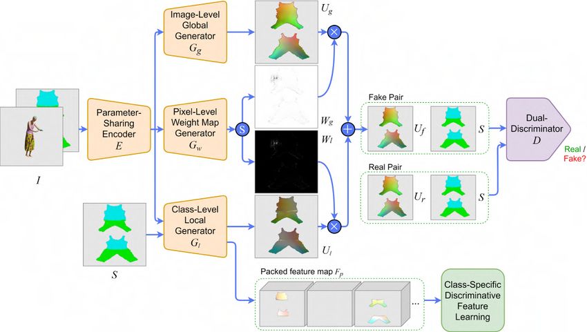
4
Acknowledgments

First of all, I would like to express my gratitude to my supervisors Meysam and
Sergio for the opportunity to work with their group. I am very grateful for the
supervision and expertise of Meysam Madadi, established researcher of the Human
Pose Recovery and Behavior Analysis (HuPBA) group. His implication, as well as
all the help and advice provided, have been key for the development of the project.
The results obtained are the fruit of countless meetings and discussions with him.
This master thesis would also not have been possible without the direction of
Sergio Escalera, expert in Computer Vision, especially in human pose recovery and
human behaviour analysis.
I would also like to thank the entire Human Pose Recovery and Behavior Analysis
(HuPBA) group and the Computer Vision Center (CVC) for providing me with
the computational resources necessary for developing the project.
In the Master in Artificial Intelligence (MAI), I have met wonderful people, good
friends and excellent professionals, who I am sure will achieve everything they
aspire to do. I want to thank them for all the support they have given me during
the development of this project and the whole master.
Finally, I cannot be more grateful to my family for their unconditional support in
everything I do. They are my rock.

                                        5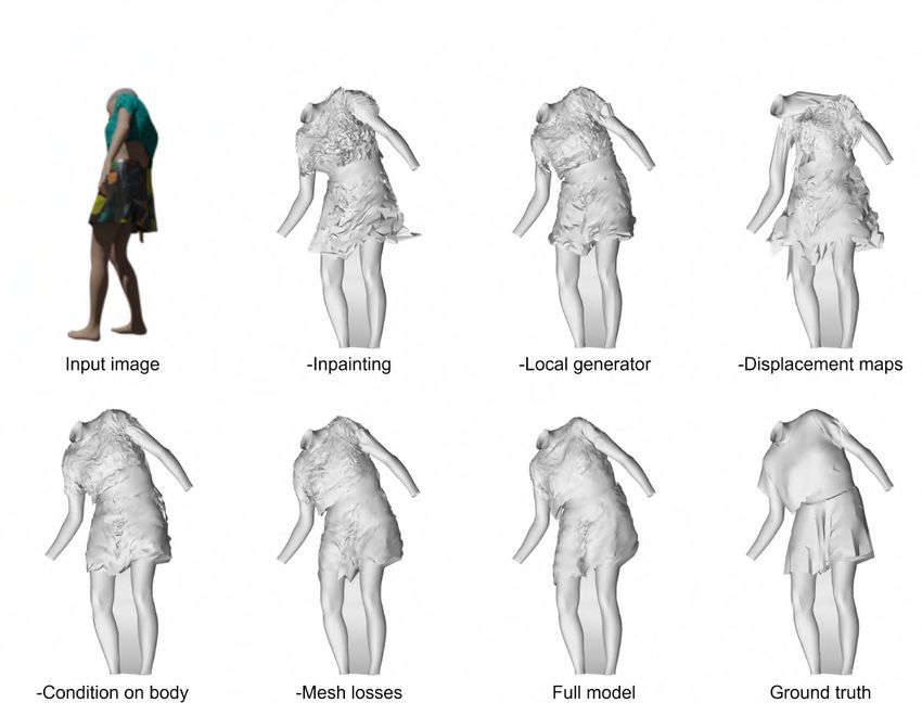
6
Contents

1 Introduction                                                                                                               13
  1.1 Motivation . . . . . . . . . . . . . . . . . . . . . . . . . . . . . . . .                                             13
  1.2 Contribution . . . . . . . . . . . . . . . . . . . . . . . . . . . . . . .                                             14
  1.3 Overview . . . . . . . . . . . . . . . . . . . . . . . . . . . . . . . . .                                             14

2 Background                                                                                                                 17
  2.1 Generative Adversarial Network . .             .   .   .   .   .   .   .   .   .   .   .   .   .   .   .   .   .   .   17
      2.1.1 Conditional GAN . . . . . .              .   .   .   .   .   .   .   .   .   .   .   .   .   .   .   .   .   .   19
  2.2 3D data representations . . . . . .            .   .   .   .   .   .   .   .   .   .   .   .   .   .   .   .   .   .   20
      2.2.1 Voxel-based representations              .   .   .   .   .   .   .   .   .   .   .   .   .   .   .   .   .   .   20
      2.2.2 Point clouds . . . . . . . . .           .   .   .   .   .   .   .   .   .   .   .   .   .   .   .   .   .   .   21
      2.2.3 3D meshes and graphs . . .               .   .   .   .   .   .   .   .   .   .   .   .   .   .   .   .   .   .   21
      2.2.4 UV maps . . . . . . . . . .              .   .   .   .   .   .   .   .   .   .   .   .   .   .   .   .   .   .   21

3 Related work                                                                                                               23
  3.1 3D reconstruction . . . . . . . . .        .   .   .   .   .   .   .   .   .   .   .   .   .   .   .   .   .   .   .   23
      3.1.1 Learning-based approaches            .   .   .   .   .   .   .   .   .   .   .   .   .   .   .   .   .   .   .   24
  3.2 Garment reconstruction . . . . .           .   .   .   .   .   .   .   .   .   .   .   .   .   .   .   .   .   .   .   26
  3.3 UV map works . . . . . . . . . .           .   .   .   .   .   .   .   .   .   .   .   .   .   .   .   .   .   .   .   28

4 Methodology                                                                                                                31
  4.1 Our UV maps . . . . . . . . . . . . . . . .                    . . .       .   .   .   .   .   .   .   .   .   .   .   31
      4.1.1 Normalise UV maps . . . . . . . .                        . . .       .   .   .   .   .   .   .   .   .   .   .   31
      4.1.2 Inpainting . . . . . . . . . . . . . .                   . . .       .   .   .   .   .   .   .   .   .   .   .   32
      4.1.3 Semantic map and SMPL body UV                            map         .   .   .   .   .   .   .   .   .   .   .   33
  4.2 LGGAN for 3D garment reconstruction . .                        . . .       .   .   .   .   .   .   .   .   .   .   .   33
      4.2.1 Architecture . . . . . . . . . . . . .                   . . .       .   .   .   .   .   .   .   .   .   .   .   34
      4.2.2 3D loss functions . . . . . . . . . .                    . . .       .   .   .   .   .   .   .   .   .   .   .   40

5 Experiments and Results                                                                                                    43
  5.1 Dataset . . . . . . . . . . . . .      .   .   .   .   .   .   .   .   .   .   .   .   .   .   .   .   .   .   .   .   43
  5.2 Experimental setup . . . . . . .       .   .   .   .   .   .   .   .   .   .   .   .   .   .   .   .   .   .   .   .   45
      5.2.1 Training details . . . . .       .   .   .   .   .   .   .   .   .   .   .   .   .   .   .   .   .   .   .   .   45
      5.2.2 Evaluation metrics . . .         .   .   .   .   .   .   .   .   .   .   .   .   .   .   .   .   .   .   .   .   47
  5.3 Results . . . . . . . . . . . . . .    .   .   .   .   .   .   .   .   .   .   .   .   .   .   .   .   .   .   .   .   48
      5.3.1 Normalisation techniques         .   .   .   .   .   .   .   .   .   .   .   .   .   .   .   .   .   .   .   .   48
      5.3.2 Inpainting UV maps . .           .   .   .   .   .   .   .   .   .   .   .   .   .   .   .   .   .   .   .   .   49

                                         7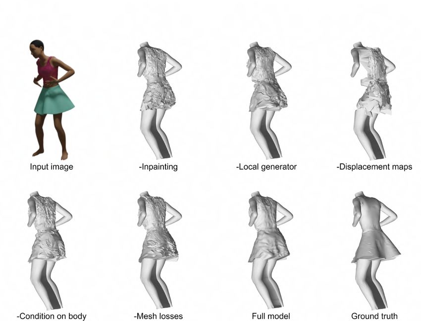
8 CONTENTS
5.3.3 Semantic map vs Body UV map conditioning . . . . . . . . 50
5.3.4 Removing local generation branch . . . . . . . . . . . . . . . 51
5.3.5 3D mesh losses . . . . . . . . . . . . . . . . . . . . . . . . . 52
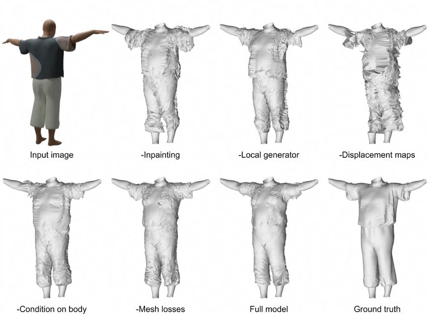
5.4 Ablation study . . . . . . . . . . . . . . . . . . . . . . . . . . . . . 54
5.4.1 Quantitative analysis . . . . . . . . . . . . . . . . . . . . . . 54
5.4.2 Qualitative analysis . . . . . . . . . . . . . . . . . . . . . . . 55
5.5 Comparison with SOTA . . . . . . . . . . . . . . . . . . . . . . . . 58
6 Conclusions and future work 59
Bibliography 61
List of Figures
2.1 GAN architecture . . . . . . . . . . . . . . . . . . . . . . . . . . . . 17
2.2 Conditional GAN architecture . . . . . . . . . . . . . . . . . . . . . 20
2.3 UV map example . . . . . . . . . . . . . . . . . . . . . . . . . . . . 22
2.4 Cube UV mapping/unwrapping . . . . . . . . . . . . . . . . . . . . 22
4.1 Original UV map vs Inpainted UV map . . . . . . . . . . . . . . . . 32
4.2 Semantic segmentation map and SMPL body UV map . . . . . . . 33
4.3 LGGAN overview . . . . . . . . . . . . . . . . . . . . . . . . . . . . 34
4.4 LGGAN overview - Conditioning on SMPL body UV map . . . . . 35
4.5 Parameter-Sharing Encoder . . . . . . . . . . . . . . . . . . . . . . 36
4.6 Class-Specific Local Generation Network . . . . . . . . . . . . . . . 37
4.7 Deconvolutional and convolutional blocks architecture . . . . . . . . 38
4.8 Class-Specific Discriminative Feature Learning . . . . . . . . . . . . 39
5.1 CLOTH3D sequence example . . . . . . . . . . . . . . . . . . . . . 44
5.2 CLOTH3D garment type examples . . . . . . . . . . . . . . . . . . 44
5.3 CLOTH3D dress samples . . . . . . . . . . . . . . . . . . . . . . . . 44
5.4 CLOTH3D subset garment type distribution . . . . . . . . . . . . . 45
5.5 Original image vs Pre-processed image . . . . . . . . . . . . . . . . 46
5.6 Normalisation techniques reconstruction examples . . . . . . . . . . 49
5.7 Inpainting technique reconstruction example . . . . . . . . . . . . . 50
5.8 Conditioning approaches reconstruction examples . . . . . . . . . . 51
5.9 Local generation network contribution example . . . . . . . . . . . 52
5.10 Attention local weight map example . . . . . . . . . . . . . . . . . . 53
5.11 3D mesh losses contribution example . . . . . . . . . . . . . . . . . 53
5.12 Ablation study on a T-shirt+Skirt sample . . . . . . . . . . . . . . 56
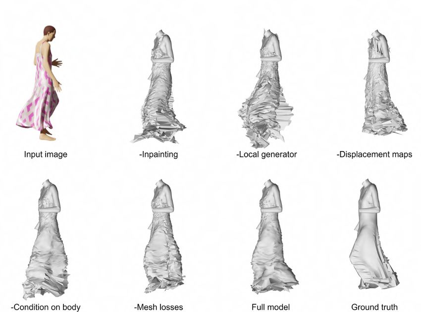
5.13 Ablation study on a Dress sample . . . . . . . . . . . . . . . . . . . 57
5.14 Ablation study on a T-shirt+Trousers sample . . . . . . . . . . . . 57
5.15 Ablation study on a Top+Skirt sample . . . . . . . . . . . . . . . . 58
9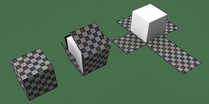
10                                                                            LIST OF TABLES

List of Tables

     5.1   Normalisation experiment evaluation . . . . .      .   .   .   .   .   .   .   .   .   .   .   .   49
     5.2   Inpainting experiment evaluation . . . . . . .     .   .   .   .   .   .   .   .   .   .   .   .   50
     5.3   Conditioning map experiment evaluation . . .       .   .   .   .   .   .   .   .   .   .   .   .   51
     5.4   Local generation branch experiment evaluation      .   .   .   .   .   .   .   .   .   .   .   .   52
     5.5   Mesh losses experiment evaluation . . . . . . .    .   .   .   .   .   .   .   .   .   .   .   .   54
     5.6   Ablation study . . . . . . . . . . . . . . . . .   .   .   .   .   .   .   .   .   .   .   .   .   55
     5.7   S2S comparison against SOTA . . . . . . . . .      .   .   .   .   .   .   .   .   .   .   .   .   58
Glossary
CV: Computer Vision
DL: Deep Learning
AI: Artificial Intelligence
GAN: Generative Adversarial Network
CGAN: Conditional Generative Adversarial Network
Local Class-Specific and Global Image-Level Generative Adversarial
LGGAN:
Network
SMPL: Skinned Multi-Person Linear model
1112
1.      Introduction

This master thesis tries to find a proper system to learn garment dynamics and
reconstruct 3D garment models from single RGB images. We present a model
based on Generative Adversarial Networks (GANs) [16] that has the peculiarity
to use UV maps to represent 3D data. We study the feasibility of this type of
representations for 3D reconstruction and generation tasks.
The GAN model used is based on LGGAN (Local Class-Specific and Global
Image-Level Generative Adversarial Networks) [56], used previously on semantic-
guided scene generation tasks like cross-view image translation and semantic image
synthesis and characterised by combining two levels of generation, global image-level
and local class-specific.

1.1    Motivation
Inferring 3D shapes from a single viewpoint is an essential human vision feature
extremely difficult for computer vision machines. For this reason, there has always
been a great deal of research devoted to building 3D reconstruction models capable
of inferring the 3D geometry and structure of objects or scenes from a single or
multiple 2D pictures. Tasks in this field go from reconstructing objects like cars or
chairs to modelling entire cities. These models can be used for a wide variety of
applications such as 3D printing, simulation of buildings in the civil engineering
field, or generation of artificial objects, humans and scenes for videogames and
movies.
One field in which the research community and industry have been working for
years has been the study of human dynamics. Accurately tracking, capturing,
reconstructing and animating the human body, face and garments in 3D are
critical tasks for human-computer interaction, gaming, special effects and virtual
reality. Despite the advances in the field, most research has concentrated only on
reconstructing unclothed bodies and faces, but modelling and recovering garments
have remained notoriously tricky.
For this reason, our work plans to push the research on the specific domain of
garments, learning clothing dynamics and reconstructing clothed humans. As said,
this is still a quite new research area, but with also many potential applications and
benefits: allow virtual try-on experiences when buying clothes, reduce designers
and animators workload when creating avatars for games and movies, etc.
First-generation methods that tried to recover the lost dimension from just 2D
images were concentrated on understanding and formalising, mathematically, the 3D

                                         13
14 CHAPTER 1. INTRODUCTION to 2D projection process [20, 31]. However, this kind of solutions required multiple images captured with well-calibrated cameras and, in some cases, accurately segmented, which in many cases is not possible or practical. Surprisingly, humans can easily estimate the approximate size and geometry of objects and imagine how they would be from a different perspective with just one image. We are able to do so because of all previously witnessed items and scenes, which have allowed us to acquire prior knowledge and construct mental models of how objects look like. The most recent 3D reconstruction systems developed have attempted to leverage this prior knowledge by formulating the problem as a recognition problem. Recent advances in Deep Learning (DL) algorithms, as well as the increasing availability of large training datasets, have resulted in a new generation of models that can recover 3D models from one or multiple RGB images without the complex camera calibration process. In this project, we are interested in these advantages, so we focus on developing a solution of this second category, using and testing different Deep Learning techniques. In contrast to other models, our solution has the peculiarity of using UV maps as 3D representation. Compared to other representations such as meshes, point clouds or voxel-based representations, which are the ones commonly used in other 3D Deep Learning models [11, 13, 17, 19, 33, 38, 44, 45, 47, 57, 61–63, 65], UV maps allow us to use standard computer vision (CV) architectures, usually intended for images and two-dimensional inputs/outputs. In addition, and even more important, UV maps are lightweight and capable of modelling fine details, a feature necessary for modelling challenging dynamic systems like garments. 1.2 Contribution The main contribution of this thesis is the proposal of a system that can adequately learn garment dynamics and reconstruct clothed humans from a single RGB image, using UV maps to represent 3D data and achieving state-of-the-art results in CLOTH3D [4] dataset. In addition, this work also studies the feasibility and impact of using UV map representations for 3D reconstruction tasks, demonstrating that it is an interesting option that could be applied in many other tasks. Finally, this project proposes and studies different strategies and techniques to perform this kind of task, and analyses quantitatively and qualitatively their contribution to our final solution. 1.3 Overview Apart from this first chapter, where we introduced our work, the rest of the thesis is split into five more parts. In the next chapter, Chapter 2, we detail all the required theoretical background needed to have a complete understanding of the project. In Chapter 3 we describe the related work and present similar works done in the current state-of-the-art.
1.3. OVERVIEW                                                                  15

Following, in Chapter 4 we extensively detail and present our proposal. Chapter
5 describes the dataset used for training and testing our model and shows all
the experiments done and the results obtained, which are discussed and analysed
quantitatively and qualitatively. Finally, in Chapter 6 we present the conclusions
about this work and ideas for future work.
16 CHAPTER 1. INTRODUCTION
2.      Background

This chapter presents the relevant background required to understand the followed
methodology. First, it introduces the GAN architecture in which our model is
based and then the different data representations usually used to represent 3D
data, with an emphasis on UV maps, the representation used in our project.

2.1    Generative Adversarial Network
A Generative Adversarial Network (GAN) [16], designed in 2014 by Ian J. Good-
fellow et al ., is a deep neural network framework that, given a set of training data,
learns to generate new data with the same properties/statistics as the training
data.
Indeed GAN architecture (Figure 2.1) is composed of two deep networks, a generator
and a discriminator, which compete against each other.
   • Generator: learns to generate realistic fake samples from a random seed. The
     generated instances produced are used as negative training examples for the
     discriminator.
   • Discriminator: learns to distinguish real samples from fake ones (coming from
     the generator).

           Figure 2.1: Generative Adversarial Network architecture. Source: [70]

The competition between both parts in this two-player game drives the whole
model to improve until fake samples are good enough they cannot be distinguished

                                            17
18 CHAPTER 2. BACKGROUND
from real ones. To have a good generative model, both networks must perform well.
If the generator is not good enough, it will not be able to fool the discriminator, and
the model will never converge. On the other hand, if the discriminator performance
is poor, then any sample will be labelled as real, even if it does not approximate
the training data distribution, which means the model will never learn.
In the beginning, the generator’s fake output is very easy for the discriminator to
differentiate from the real data. Over time, the generator’s output will become more
realistic, and the generator will get better at fooling the discriminator. Eventually,
the generator will generate such realistic outputs that the discriminator will be
unable to distinguish them. In fact, for a perfect generator, the discriminator
should have only 50% of accuracy, being completely random. Training the model
beyond this convergence point could cause the discriminator to give wrong feedback
to the generator, decreasing its performance.
To generate fake samples, the generator G receives as input some noise z, sampled
using a normal or uniform distribution. Conceptually, this z represents the latent
features of the samples generated, which are learned during the training process.
Latent features are those variables that cannot be observed directly but are
important for a domain. It can also be seen as a projection or compression of data
distribution, providing high-level concepts of the observed data. This generator
typically consists of multiple transposed convolutions that upsample vector z.
Once the synthetic samples G(z) are generated, they are mixed together with real
examples x coming from the training data and forwarded to the discriminator
D, who classifies them as fake or real. The loss function of the discriminator is
computed based on how accurate is its assessment and the hyperparameters are
adjusted in order to maximise its accuracy. This loss is described formally in
Equation 2.1, and it is composed of two terms: the first one rewards the recognition
of real samples (log D(x)), and the second one the recognition of generated samples
(log(1 − D(G(z)))). On the other hand, the generator is rewarded or penalised
based on how well or not the generated samples fool the discriminator. Its objective
function is shown in Equation 2.2, and it wants to optimise G so it can fool the
discriminator D the most, generating samples with the highest possible value of
D(G(z)). This two-player minimax game can also be formalised with just one
single value function V (G, D), shown in Equation 2.3, which the discriminator
wants to maximise and the generator minimise.
max V (D) = Ex∼pdata (x) [log D (x)] + Ez∼pz (z) [log (1 − D (G (z)))] (2.1)
D
min V (G) = Ez∼pz (z) [log (1 − D (G (z)))] (2.2)
G
min max V (D, G) = Ex∼pdata (x) [log D (x)] + Ez∼pz (z) [log (1 − D (G (z)))] (2.3)
G D
being D(x) the estimated probability that an input example x is real, Ex∼pdata (x)
the expected value over all examples coming from training data, G(z) the fake
example produced by the generator for the random noise vector z, D(G(z)) the2.1. GENERATIVE ADVERSARIAL NETWORK 19
estimate by the discriminator of the probability that a fake input example G(z) is
real, and Ez∼pz (z) the expected value over all random inputs to the generator.
These objective functions are learned jointly by the alternating gradient descent.
In each training iteration, we first fix the generator weights and perform k training
steps on the discriminator using generated samples, coming from the generator,
and the real ones, coming from the training set. Then, we fix the discriminator
parameters and we train the generator for a single iteration. We keep training
both networks in alternating steps until we think the model has converged and the
generator produces good quality samples. This training process can be formalised
with the following pseudocode Algorithm 2.1:
Algorithm 2.1 GAN training
1: for number of training iterations do
2: for k steps do
3: Sample minibatch of m noise samples z(1), ..., z (m) from noise prior pg (z)
4: Sample minibatch of m examples x(1), ..., x(m) from data generating
distribution pdata (x)
5: Update the discriminator D by ascending its stochastic gradient:
1 Pm (i) + log 1 − D G z (i)
∇θd m i=1 log D x
6: end for
7: Sample minibatch of m noise samples z(1), ..., z (m) from noise prior pg (z)
8: Update the generator G by descending its stochastic gradient:
1 Pm (i)
∇ θg m i=1 log 1 − D G z
9: end for
As during early training, the discriminator D typically wins against the generator
G, the gradient of the generator tends to vanish and makes the gradient descent
optimisation to be very slow. To speed it up, the GAN authors proposed to, rather
than training G to minimise log(1 − D(G(z))), train it to maximise log D(G(z))
2.1.1 Conditional GAN
Conditional Generative Adversarial Networks (CGANs) [39] are an extension of the
GANs in which the generator and discriminator are conditioned by some additional
input y. This new input can be of any kind (class labels or any other property) and
is usually feed into both the discriminator and generator as an additional input
layer, concatenating input noise z and condition value y, as can be seen in Figure
2.2.
With this modification, the objective function of the Conditional GAN can be
expressed as follows:
min max V (D, G) = Ex∼pdata (x) [log D (x|y)] + Ez∼pz (z) [log (1 − D (G (z|y)))]
G D
(2.4)
The motivation behind the conditioning is to have a mechanism to request the
generator for a particular input. For example, suppose we train a GAN to generate20 CHAPTER 2. BACKGROUND
Figure 2.2: Conditional Generative Adversarial Network architecture. Source: [70]
new MNIST images [32], which is a very well-known dataset of handwritten digits.
In that case, we will have no control over what specific digits will be produced by
the generator. However, if we input to a Conditonal GAN the handwritten digit
image together with its class label (number appearing in the image), the generator
will learn to generate numbers based on their class and we will be able to control
its output.
2.2 3D data representations
Computer Vision (CV) and Deep Learning (DL) research has typically focused on
working with 2D data, images and videos. Recently, with the availability of large
3D datasets and more computational power, the study and application of Deep
Learning techniques to solve tasks on 3D data has grown a lot. These tasks include
segmentation, recognition, generation and reconstruction, among others. However,
as there is no single way to represent 3D models, the 3D datasets available in
the current state-of-the-art are found in a wide variety of forms, varying in both
structure and properties.
In this section, we give an overview of the most common 3D representations used
in Deep Learning architectures (point clouds, 3D meshes, voxels and RGB-D data)
and the type of representation used and evaluated in this project (UV maps),
detailing their differences and the challenges of each one.
2.2.1 Voxel-based representations
One voxel is basically a 3D base cubical unit that, together with other voxels, form
a 3D object inside a regular grid in the 3D space. It can be seen as a 3D extension
of the concept of pixel.
The main limitation of voxels is their inefficiency to represent high-resolution data,
as they represent both occupied and non-occupied parts of the scene, needing an
enormous amount of memory for non-occupied parts. Using a more efficient 3D
volumetric representation such as octree-based, which consists basically of varying-
sized voxels, one can represent higher resolution objects with less computation2.2. 3D DATA REPRESENTATIONS 21
consumption, thanks to their ability to share the same voxel for large regions of
space. Despite this, both voxels and octree representations do not preserve the
geometry of 3D objects, in terms of the shape and surface smoothness, and lack of
enough detail, reason why they are not adequate in all domains.
2.2.2 Point clouds
A 3D point cloud is a set of unstructured data points in a three-dimensional
coordinate system that approximates the geometry of 3D objects. These points
are defined using x, y, z coordinates and are usually obtained by 3D scanners like
LiDAR or photogrammetry [64].
Point-based representations are simple and efficient, but, as they are not regular
structures, they do not fit into convolutional architectures that exploit spatial
regularity. To get around this constraint, the following representations emerged:
• Point set representation, which treats a point cloud as a matrix of size N × 3,
being N the number of points.
• 3-channel grids of size H ×W ×3, encoding in each pixel the x, y, z coordinates
of a point.
• Depth maps from multiple viewpoints.
However, the lack of structure, caused by the absence of connectivity information
between point clouds, results in an ambiguity about the surface information. In
the domain of garments, this problem means that wrinkles cannot be handled
properly, even if the number of points is very high.
2.2.3 3D meshes and graphs
Meshes are one of the most popular representations used for modelling 3D objects
and shapes. A 3D mesh is a geometric data structure that allows the representation
of surface subdivisions by a set of polygons. These polygons are called faces and are
made up of vertices. The vertices describe how the mesh coordinates x, y, z exist in
the 3D space and connect to each other forming the faces. Most commonly, these
faces are triangles (triangular meshing), but there also exist quadrilateral meshes
and volumetric meshes, which connect the vertices by tetrahedrons, pyramids,
hexahedrons or prisms [64].
The challenge with this kind of representation is that Deep Learning algorithms
have not been readily extended to such irregular representations. For this reason,
it has become common to use graph-structured data to represent 3D meshes and
use Graph Convolutional Networks (GCN) to process them. In these graphs, the
nodes correspond to the vertices and the edges the connectivity between them.
Using these graphs, has opened the door to the creation and innovation of Deep
Learning models based on this kind of graph convolutions.
2.2.4 UV maps
A UV map is the flat representation of the surface of a 3D model, usually used to
wrap textures easily and efficiently. The letters U and V refer to the horizontal22 CHAPTER 2. BACKGROUND
and vertical axes of the 2D space, as X, Y and Z are already used to denote the
axis of the 3D space. Basically, in a UV map, each of the 3D coordinates/vertices
of the object is mapped into a 2D flat surface.
Below, in Figure 2.3, we show an example of a 3D model (right) and its corre-
sponding unwrapped surface on a UV map (left).
Figure 2.3: Example of a 3D face model and its corresponding UV map. Source: [58]
The process of creating a UV map is called UV unwrapping and consists of assigning
to each 3D vertex (X, Y, Z) their corresponding UV coordinate. Thus, UV maps
act as marker points that determine which points (pixels) on the texture correspond
to which points (vertices) on the mesh. The inverse process, projecting the UV
map onto a 3D model’s surface, is called UV mapping.
Figure 2.4: Representation of the UV mapping/unwrapping of a cube. Source: [58]
The main benefit of it is that it is a flat representation (2D), so it can be used in
standard Computer Vision models thought for images or videos. Therefore one can
take advantage of all the advances already done in Computer Vision for 2D data,
which, as said before, is where there is more research and focus. Besides this, it is
also a lightweight representation and can handle fine details, suitable for dealing
with garment wrinkles.3. Related work
After explaining and contextualising the necessary background, in this chapter
we describe the works that are most related to our approach. First, we explain
the leading works in the state-of-the-art of image-based 3D object reconstruction.
Then we go into the specific domain of garments, presenting different solutions
that reconstruct 3D garment models from single or multiple images. Finally, we
give an overview of other works that also use and study UV map representations.
3.1 3D reconstruction
Fast and automatic 3D object reconstruction from 2D images is an active research
area in Computer Vision with an increasing interest coming from many industries
and applications: e-commerce, architecture, game and movie industries, automotive
sector, 3D printing. For this reason, during the last decades, a large amount of
work has been carried out on this topic, from reconstructing objects like chairs,
cars or planes to modelling faces, scenes, or even entire cities.
The first works done approached the problem from a geometric perspective and
tried to understand and formalise the 3D projection process mathematically. It is
the case of techniques based on the multi-view geometry (MVG) [20], also known
as stereo-based techniques, that match features across the images from different
views and use the triangulation principle to recover 3D coordinates. Although
these solutions are very successful in some scenarios such as structure from motion
(SfM) [53] for large-scale high-quality reconstruction and simultaneous localisation
and mapping (SLAM) [9] for navigation, they are subject to several restrictions:
they need to have a great number of images from different viewpoints of the object,
and this cannot be non-lambertian (e.g. reflective or transparent) nor textureless.
If the number of images is not enough or they do not cover the entire object, MVG
will not reconstruct the unseen parts as it will not be able to establish feature
correspondences between images. The lack of textures and reflections also affect
this feature matching [5, 51].
With the aim of being able to reconstruct non-lambertian surfaces, shape-from-
silhouette, or shape-by-space-carving, methods [31] appeared and became popular.
However, these methods require the objects to be accurately segmented from the
background or well-calibrated cameras, which is not suitable in many applications.
All these restrictions and disadvantages lead the researchers to draw on learning-
based approaches, that consider single or few images and rely on the shape prior
knowledge learnt from previously seen objects. Early works date back to Hoiem
2324 CHAPTER 3. RELATED WORK et al . [22] and Saxena et al . [52]. Nevertheless, it was not until recently, with the success of Deep Learning architectures, and more importantly, the release of large-scale 3D datasets such as ShapeNet [10], that learning-based approaches achieved great progress and very exciting and promising results. This section provides an overview of some of the most important and well-known 3D reconstruction models belonging to this latter family. 3.1.1 Learning-based approaches As explained in Chapter 2, unlike 2D images, which are always represented by regular grids of pixels, 3D shapes have various possible representations, being voxels, point clouds and 3D meshes the most common. This has led to 3D reconstruction models that are very different from each other, as their architectures largely depend on the representation used. For this reason, we review the most relevant works of each of these types of representation, giving an overview of their architecture and characteristics. 3.1.1.1 Voxel-based Voxel-based representations were among the first representations used with Deep Learning techniques to reconstruct 3D objects from images. This is probably due to their 2D analogy, pixels, a data type that has been used in computer vision for decades. Because of this, during the last few years, many different approaches dealing with this representation have appeared, each one attempting to outperform the preceding and pushing the state-of-the-art. 3D-R2N2 3D Recurrent Reconstruction Neural Network, usually called just 3D- R2N2 [11] is a recurrent neural network architecture designed by Choy et al . that unifies both single and multi-view 3D object reconstruction problems. The framework takes in one or more images of an object from different perspectives to learn a 3D reconstruction of it. The network can perform incremental refinements and adapt as new viewpoints of the object become available. It is an encoder- decoder architecture composed of mainly three modules: a 2D Convolutional Neural Network (2D-CNN), a 3D Convolutional LSTM (3D-LSTM) and a 3D- Deconvolutional Neural Network (3D-DCNN). The 2D-CNN is in charge of encoding the input images into features. Then, given these encoded features, a set of 3D- LSTM units selects either to update their cell states or retain them by closing the input gate, allowing the network to update the memory with new images or retain what it has already seen. Finally, the 3D-DCNN decodes the hidden states of the 3D-LSTM units, generating a 3D probabilistic voxel reconstruction. 3D-VAE-GAN With the success of GANs [16] and variational autoencoders (VAEs) [27], Wu et al . [63] presented 3D-VAE-GAN, inspired by VAE-GAN [30]. This model applies GANs and VAEs in voxel data to generate 3D objects from just one single-view image. It is composed of an encoder that infers a latent vector z from the input 2D image and a 3D-GAN, which learns to generate the 3D object from the latent space vector z by using volumetric convolutional networks.
3.1. 3D RECONSTRUCTION                                                            25

Octree Generating Networks Due to the high computational cost of voxel-based
representations, the methods described before cannot cope with high-resolution
models. For this reason, Tatarchenko et al . [57] proposed the Octree Generating
Networks (OGN), a deep convolutional decoder architecture that can generate
volumetric 3D outputs in an efficient manner by using octree-based representations,
being able to manage relatively high-resolution outputs with a limited memory
budget. In OGN, the representation is gradually convolved with learnt filters and
up-sampled, as in a traditional up-convolutional decoder. However, the novelty
of it is that, starting from a certain layer in the network, dense regular grids
are replaced by octrees. As a result, the OGN network predicts large regions of
the output space early in the first decoding stages, saving computation for the
subsequent high-resolution layers.

Pix2Vox     Recently, to overcome the limitations of solutions that use recurrent
neural networks (RNNs) like 3D-R2N2 [11], Xie et al . [65] introduced Pix2Vox
model. The main restrictions of models based on recurrent networks are the
time consumption, since input images cannot be processed in parallel, and the
inconsistency between predicted 3D shapes of two sets containing the same input
images but processed in a different order. For this reason, the authors of Pix2Vox
proposed a model composed of multiple encoder-decoder modules running in
parallel, each one predicting a coarse volumetric grid from its input image frame.
These different predicted coarse 3D modules are merged in a fused reconstruction
of the whole object by a multi-scale context-aware fusion model, which selects
high-quality reconstructions. Finally, a refiner corrects the wrongly recovered parts
generating the final reconstruction.

3.1.1.2   Point-based

Similar to the works using volumetric-based representations, models that use point-
based representations follow an encoder-decoder model. In fact, all of them use the
same architecture for the encoder but differ in the decoder part. The works that
use point sets to represent point clouds use fully connected layers on the decoder,
since point clouds are unordered, while the ones that use grids or depth maps use
up-convolutional networks.

Point Set Generation Network Fan et al . [13] presented a network that combines
both point set and grid representations, composed of a cascade of encoder-decoder
blocks. Each block takes the output of its previous block and encodes it into a
latent representation that is then decoded into a 3-channel image. The first block
takes as input the image. The last block has an encoder followed by a predictor
of two branches: a decoder that predicts a 3-channel image, being each pixel the
coordinates of a point, and a fully-connected network that predicts a matrix of size
N × 3, being each row a 3D point. To output the final prediction, the predictions
of both branches are merged using a set union.

DensePCR As the network mentioned above and its variants are only able to
recover low-resolution geometry, Mandikal et al . [38] presented DensePCR, a
26                                                CHAPTER 3. RELATED WORK

framework composed of a cascade of multiple networks capable of handling high
resolutions. The first network of the cascade predicts a low-resolution point cloud.
Then, each subsequent block receives as input the previously predicted point cloud
and computes global features, using a multi-layer perceptron architecture (MLP)
similar to PointNet [44] and PointNet++ [45], and local features, using MLPs in
balls surrounding each point. These global and local features are combined and
fed to another MLP, which predicts a dense point cloud. This procedure can be
repeated as many times as necessary until the desired resolution is achieved.

3.1.1.3    Mesh-based

The last most common used representation in 3D reconstruction models are 3D
meshes. Compared to point-based representations, meshes contain connectivity
information between neighbouring points, making them better for describing local
regions on surfaces.

Pixel2Mesh      Wang et al . proposed Pixel2Mesh [61], an end-to-end Deep Learning
architecture designed to produce 3D triangular meshes of objects given just a single
RGB image. Their approach is based on the gradual deformation of an ellipsoid
mesh with a fixed size to the target geometry. To do so, they use Graph-based
Convolutional Networks (GCNs) and refine the predicted shape gradually using a
coarse-to-fine fashion, increasing the number of vertices as the mesh goes through
the different stages. This network outperforms 3D-R2N2 framework, as the latter
lacks of details due to the low resolution that voxel-based representations allow.
Wen et al . [62] extended Pixel2Mesh and proposed Pixel2Mesh++, which ba-
sically allows reconstructing the 3D shapes from multi-view images. To do so,
Pixel2Mesh++ presents a Multi-view Deformation Network (MDN) that incorpo-
rates the cross-view information into the process of mesh generation.

AtlasNet    Another generative model for mesh-based representations is AtlasNet,
proposed by Groueix et al . [17], but with a totally different approach. AtlasNet
decomposes the surface of a 3D object into m patches and learns to convert 2D
square patches into 2-manifolds to cover the surface of the 3D shape (Papier-Mâché
approach) by using a simple Multi-Layer Perceptron (MLP). The designed decoder
is composed of m branches, and each branch is in charge of reconstructing a
different patch. Then, these reconstructed patches are merged together to form
the entire surface. Its main limitation is, however, that the number of patches m
is a parameter of the system and its optimal number depends on each surface and
object, making the model not general enough.

3.2       Garment reconstruction
If inferring 3D shapes of simple and static objects like chairs or cars from a single
image is already complicated, doing so for 3D cloth models is extremely challenging.
Garments are not only very dynamic objects but also belong to a domain where
there is a huge variety of topologies and types.
3.2. GARMENT RECONSTRUCTION                                                          27

Early works focused on garment modelling from images approached the problem
from a geometric perspective [8, 24, 68]. Then, the advent of deep learning achieved
impressive progress in the task of reconstructing unclothed human shape and pose
from multiple or single images [7, 25, 28, 29, 42, 43, 54, 66]. Nevertheless, recovering
clothed human 3D models did not progress in the same way, not only because
of the challenges mentioned before but also as a consequence of the lack of large
annotated training datasets available.
It is only recently, in the last few years, that new large datasets and deep learning
works focused on this domain started to emerge, trying to push its state-of-the-art.
A standard practice used in garment reconstruction frameworks is to represent
garments as an offset over the Skinned Multi-Person Linear model (SMPL) body
mesh [1, 6], which is a skinned vertex-based model that accurately represents a
wide variety of body shapes in natural human poses [34]. However, this type of
approach has the disadvantage that it may fail for loose-fitting garments, which have
significant displacements over the shape of the body. For this reason, there are works
that use non-parametric representations such as voxel-based representations [60],
visual hulls [40] or implicit functions [12, 49, 50]. Finally, there are also some works
that have combined both parametric and non-parametric representations [23,67,69].

Below, we analyse the characteristics and contributions of some of these deep
learning frameworks.

Multi-Garment Net        Multi-Garment Network (MGN) [6] designed by Bhatnagar
et al . in 2019 is a network that reconstructs body shape and clothing, layered on
top of the SMPL model, from a few frames of a video. It was the first model that
was able to recover separate body shape and clothing from just images.
The model introduces class-specific garment networks, each one dealing with a
particular garment topology. Despite this, because of the very limited dataset used,
presented in the same work, with just a few hundreds of samples, each branch is
prone to overfitting issues. Furthermore, as MGN relies on pre-trained parametric
models, it is unable to handle out-of-scope deformations. Moreover, it typically
requires eight frames as input to generate good quality reconstructions.

Octopus Also, in 2019, Alldieck et al . [1] presented Octopus, a learning-based
approach to infer the personalised 3D shape of people, including hair and clothing,
from few frames of a video.
It is a CNN-based method that encodes the frames of the person (in different
poses) into latent codes that then are fused to obtain a single shape code. This
code is finally fed into two different networks, one that predicts the SMPL shape
parameters and other that predicts the 3D vertex offsets of the garment.
As the Multi-garment net framework [6], Octopus expresses the garment as an
offset over the SMPL body mesh of the human, approach that, as mentioned before,
fails in some types of garments that are not tight to the body, like dresses or skirts.
28                                                 CHAPTER 3. RELATED WORK

PIFu    To be able to handle these clothes that largely depart from the body
shape defined by the SMPL, Pixel-aligned Implicit Function (PIFu) [49] authors
presented a kind of representation based on implicit functions that locally aligns
pixels of 2D images with the global context of their corresponding 3D object.
This representation does not explicitly discretise the output space but instead
regresses a function that determines the occupancy for any given 3D location.
This approach can handle high-resolution 3D geometry without having to keep a
discretised representation in memory.
In this work, the authors also proposed an end-to-end deep learning method that
uses PIFu representation for digitising highly detailed clothed humans that can
infer both 3D surface and texture from one or multiple images.
More recently, the same authors presented PIFuHD [50], a multi-level framework
also based on PIFu representation, which can infer 3D geometry of clothed humans
at an unprecedentedly high 1k image resolution.

Deep Fashion3D In Deep Fashion3D work [69], the authors presented a novel
large dataset to push the research in the task of garment reconstruction from just one
single image. Apart from the dataset, the authors proposed a novel reconstruction
framework that takes advantage of both meshes and implicit functions by using a
hybrid representation.
As the methods based on implicit functions showed a great ability to manage
fine geometric details, authors proposed transferring the high-fidelity local details
learned from them to a template mesh, which adapts its topology to fit the input
image’s clothing category has robust global deformations.
By using this combined representation, the model is able to handle finer details
and out-of-scope deformations.

3.3    UV map works
Within the research of garment modelling, there are a few works that have already
used UV map representations in some way. For this reason, we briefly analyse their
approach, how they use UV maps and for what purpose.

DeepCloth DeepCloth [55] is a neural garment representation framework which
goal is to perform smooth and reasonable garment style transition between different
garment shapes and topologies.
To do so, they use a UV-position map with mask representation, in which the
mask denotes the topology and covering areas of the garments, while the UV map
denotes the geometry details, i.e. the coordinates of each vertex. DeepCloth maps
both the UV map and its mask information into a feature space using a CNN-based
encoder-decoder structure. Then, by changing and interpolating these features,
garment shape transition and editing can be performed.
3.3. UV MAP WORKS                                                                 29

Tex2Shape     Alldieck et al . [2] presented Tex2Shape, a framework that aims to
reconstruct high-quality 3D geometry from an image by regressing displacements
in an unwrapped UV space.
In order to do so, the input image is transformed into a partial UV texture using
DensePose [18], mapping input pixels to the SMPL model, and then translated
by Tex2Shape network into normal and displacement UV maps. The normal map
contains surface normals, while the vector displacement map contains 3D vectors
that displace the underlying surface. Both normals and displacements are defined
on top of the body SMPL model.
With this workflow, the reconstruction problem is turned into an easier 3D pose-
independent image-to-image translation task.

SMPLicit      SMPLicit [12], a concurrent work to ours, is a novel generative model
designed by Corona et al . to jointly represent body pose, shape and clothing geom-
etry for different garment topologies, while controlling other garment properties
like garment size.
Its flexibility builds upon an implicit model conditioned with the SMPL body
parameters and a latent space interpretable and aligned with the clothing attributes,
learned through occlusion UV maps.
The properties that the model aims to control are: clothing cut, clothing style, fit
(tightness/looseness) and the output representation. To learn the latent space of
the first two properties, clothing cut and style, the authors compute a UV body
occlusion map for each garment-body pair in the dataset, setting every pixel in
the SMPL body UV map to 1 if the body vertex is occluded by the garment, and
0 otherwise.
30 CHAPTER 3. RELATED WORK
4.      Methodology

In this chapter, we present the methodology followed to build our system and
reconstruct 3D garment models. First, we explain how we use UV map represen-
tations in our approach, and the pre-processing techniques and pipeline carried
out to transform them into usable and suitable inputs for our model, a step that
has proven to be of enormous importance. After that, we detail our specific model,
explaining the architecture in which it is based and the modifications made to
support our task.

4.1     Our UV maps
As explained in Chapter 2, UV maps are the flat representation of the surface of
a 3D model. They are usually used to wrap textures, being able to project any
pixel from an image to a point on a mesh surface. Nevertheless, as seen in previous
Chapter 3, UV maps can also be used to denote other properties such as normal
coordinates or vertices coordinates, since they can assign any property encoded in
a pixel to any point on a surface.
In particular, in our approach, we use UV maps that encode garment mesh vertices,
storing 3D coordinates as if they were pixels of an RGB image, together with a mask
that denotes the topology and covering areas of the garment. In this way, we achieve
a kind of representation that can be used in standard computer vision frameworks,
usually thought for 2D data like images and videos, leveraging all progress done in
this field. Moreover, unlike other representations such as volumetric representations,
UV maps are perfectly capable of handling high-frequency cloth details efficiently.
This type of representation is also used in DeepCloth [55] and Tex2Shape [2]
frameworks, which refer to it as “UV-position map with mask” and “UV shape
image” respectively.

4.1.1   Normalise UV maps
As explained above, our UV maps contain 3D coordinate vectors x, y, z that are
mapped to the garment mesh vertices. These coordinates do not have a fixed range
and can be highly variable. For this reason, since large variability on the data can
be a problem during the training of networks, getting stuck in local minima, a
common practice is to normalise or standardise these values, helping the model to
have a more stable and efficient training.
To normalise our UV maps, we propose two different approaches:

                                         31
32 CHAPTER 4. METHODOLOGY
1. Min-max normalization: the first proposal is to use the minimum and
maximum values of coordinates xmin , ymin , zmin and xmax , ymax , zmax within the
training dataset to apply a min-max normalization and normalise all values
between the range of 0 and 1.
2. Displacement UV maps: the other proposal is to do the same as other
approaches like [1, 2, 6] and represent garment vertices as an offset over the
estimated SMPL body vertices. Alldieck et al . [2] refer to this kind of UV
maps as displacement maps, because they displace the underlying body
surface. With this approach, we somehow standardise the values and obtain
a much lower variability.
4.1.2 Inpainting
A 3D mesh is a discrete representation, as it has a finite number of vertices.
Therefore, the UV maps we use are also discrete, as they are the 2D projection of
those vertices. For this reason, the UV maps have empty gaps between vertices, as
can be seen in Figure 4.1a.
To avoid these gaps and make the UV map image smoother, we use image inpainting
techniques to estimate the values of the empty spaces. Image inpainting is a form
of image restoration that is usually used to restore old and degraded photos or
repair images with missing areas. In particular, we use the Navier-Stokes based
method [3], which propagates the smoothness of the image via partial differential
equations and at the same time preserves the edges at the boundary [37]. With
this technique, we obtain a UV map like the one in Figure 4.1b.
In Chapter 5 we detail the results of an experiment that analyses the contribution
of this pre-processing step.
(a) Original UV map (b) Inpainted UV map
Figure 4.1: Comparison between the original UV map and the inpainted one, filling the empty
gaps between projected vertices.4.2. LGGAN FOR 3D GARMENT RECONSTRUCTION 33
4.1.3 Semantic map and SMPL body UV map
Last but not least, as input, the LGGAN model expects not only an RGB image
but also a condition that guides and controls it through the generation. For this
purpose, for each UV map, we estimate a semantic segmentation map S that
contains the topology of the garments and segment them in different labels/classes,
one per garment type. An example is shown in Figure 4.2a.
Another option used to condition the model is the SMPL body UV map. This body
UV map is obtained in the same way we obtain garments UV maps, by projecting
the SMPL body mesh into the 2D UV space and applying the same pre-processing
techniques. Figure 4.2b shows an example of it. The SMPL body surface is inferred
by using SMPLR [36], a deep learning approach for body estimation.
With these conditions, the model can not only reconstruct 3D garments but also
transition between different body and garment shapes and topologies.
(a) Semantic segmentation map S (b) SMPL body UV map B
Figure 4.2: Examples of the semantic segmentation maps and the SMPL body UV maps used to
condition our model. In Figure 4.2a each color represents a different garment type.
4.2 LGGAN for 3D garment reconstruction
Investigating what solution we could propose to learn garment dynamics and
reconstruct 3D garment models from single RGB images through UV map rep-
resentations, we first thought that our task could be seen as an image-to-image
translation problem. The models used for this kind of tasks learn mappings from
input images to output images. This fits our case since our input is also an image
and, although our expected output is a UV map, this has the same dimensionality
as an RGB image: H × W × 3.
However, in these image-to-image translation systems, the input and output have
pixel correspondence between them, while in our case pixels follow a very different
path from the RGB image (input) to the UV map (output). For this reason,
we searched for systems covering the cross-view image translation task proposed
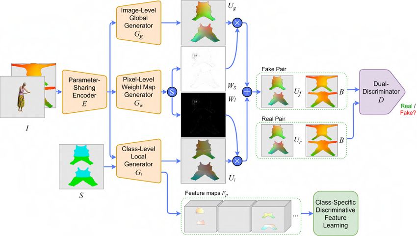
in [46], where this pixel correspondence between input and output does not exist34 CHAPTER 4. METHODOLOGY either. This task’s main goal is to generate a ground-level/street-view image from an image of the same scene but from an overhead/aerial view, and vice versa. It is a very challenging task since the information from one view usually tells very little about the other. For example, an aerial view of a building, i.e. the roof, does not give much information about the colour and design of the building seen from the street-view. As standard image-to-image translation models do not perform well on this task, recently, several specific models have emerged trying to solve this cross-view image synthesis task. One of the best works on this topic is the one published in 2020 by Tang et al . [56], in which the Local class-specific and Global image-level Generative Adversarial Networks (LGGAN) model was presented, system in which we draw from and adapt for our domain. 4.2.1 Architecture The LGGAN proposed by Tang et al . [56] is based on GANs [16], more specifically in CGANs [39], and is mainly composed of three parts/branches: a semantic-guided class-specific generator modelling local context, an image-level generator modelling the global layout, and a weight-map generator for joining the local and the global generators. An overview of the whole framework is shown in Figure 4.3. Figure 4.3: Overview of the proposed LGGAN. The symbol ⊕ denotes element-wise addition, ⊗ element-wise multiplication and s channel-wise softmax. Source: Own elaboration adapted from [56]. Like the original GAN [16], LGGAN is composed of a generator G and a discrimina- tor D. The generator G consists of a parameter-sharing encoder E, an image-level global generator Gg , a class-level local generator Gl and a weight map generator Gw . The encoder E shares parameters to all the three generation branches to make a compact backbone network. Gradients from all the three generators Gg ,
4.2. LGGAN FOR 3D GARMENT RECONSTRUCTION                                                 35

Gl and Gw contribute together to the learning of the encoder. In the original

model, the input RGB image is concatenated with a semantic map and fed to
this backbone encoder E. This semantic map is a semantic segmentation of the
target image, with a class label for every type of object appearing on it. By adding
this map, the authors somehow guide the model to learn the correspondences
between the target and source views. As explained before, in our case, we present
two different options to guide the reconstruction. The first one is conditioning in
the same way they do in the original model, by concatenating to the input RGB
image a semantic segmentation map S of the target UV map, containing a different
label/class for each garment type. The other option proposed is to condition the
class-level local generator Gl on this UV map segmentation S, but use the SMPL
body UV map B of the person to condition the image-level global generator Gg
and the discriminator D. Figure 4.2 shows examples of these inputs. Figure 4.4
presents the same LGGAN overview shown before but when conditioning also on
the SMPL body UV map B.

Figure 4.4: Overview of the proposed LGGAN when conditioning also on SMPL body UV map B.
The symbol ⊕ denotes element-wise addition, ⊗ element-wise multiplication and s channel-wise
softmax. Source: Own elaboration adapted from [56].

LGGAN extends the standard GAN discriminator to a cross-domain structure
that receives as input two pairs, each one containing a UV map and the condition
of the model. Nevertheless, the goal of the discriminator D is the same, try to
distinguish the generated UV maps from the real ones.

Finally, apart from the generator and discriminator, there is also a novel classi-
fication module responsible for learning a more discriminative and class-specific
feature representation.
36 CHAPTER 4. METHODOLOGY
4.2.1.1 Generation branches
Parameter-Sharing Encoder The first module of the network is a backbone
encoder E. This module basically takes the input I and applies several convolutions
to encode it and obtain a latent representation E(I). Its architecture is presented
in 4.5. It is composed of three convolutional blocks and nine residual blocks
(ResBlocks) [21]. Both blocks are similar and consist of convolutional layers,
instance normalisation layers and ReLU activation functions. The only difference
is that ResBlocks contain also skip connections.
Figure 4.5: Parameter-Sharing Encoder architecture. Contains three convolution blocks and nine
residual blocks. Source: Own elaboration.
Note that the input I, as explained before, is the concatenation of the input RGB
image and the condition. This condition could be either the UV map semantic
guide S or the SMPL body UV map B.
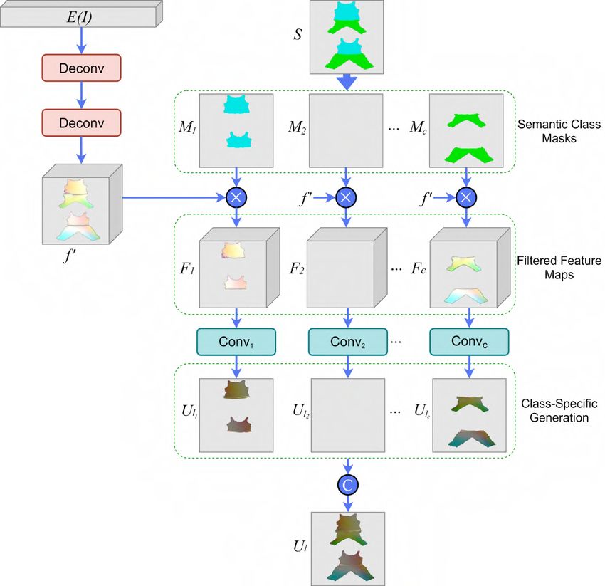
Class-Specific Local Generation Network The authors propose a novel local
class-specific generation network Gl that separately constructs a generator for
each semantic class. Each sub-generation branch has independent parameters and
concentrates on a specific class, producing better generation quality for each class
and yielding richer local details. Its overview is shown in Figure 4.6.
This generator receives as input the output of the encoder, the encoded features
E(I). These are fed into two consecutive deconvolutional blocks to increase the
spatial size. These deconvolutional blocks consist of a transposed convolution
followed by an instance normalisation layer and a ReLU activation, as shown in
Figure 4.7a. The scaled feature map f 0 is then multiplied by the semantic mask of
each class Mi , obtained from the semantic map S. By doing this multiplication,
we obtain a filtered class-specific feature map for each one of the classes. This
mask-guided feature filtering can be expressed as:
Fi = Mi · f 0 , i = 1, 2, . . . , c (4.1)
where c is the number of semantic classes (i.e. number of types of garment). After
computing these filtered feature maps, each feature map Fi is fed into a different
convolutional block, the one for the corresponding class i, which generates a class-
specific local UV map Uli . Each convolutional block is composed of a convolutional
layer and a Tanh activation function, as shown in Figure 4.7b. The loss used inYou can also read