Analysis of Performance Measures affecting the economic success on the PGA Tour using multiple linear regression - JOHANNES HÖGBOM AUGUST REGNELL ...
←
→
Page content transcription
If your browser does not render page correctly, please read the page content below
EXAMENSARBETE INOM TEKNIK,
GRUNDNIVÅ, 15 HP
STOCKHOLM, SVERIGE 2020

Analysis of Performance Measures
affecting the economic success on
the PGA Tour using multiple linear
regression

JOHANNES HÖGBOM

AUGUST REGNELL

KTH
SKOLAN FÖR TEKNIKVETENSKAP

Analysis of Performance Measures
affecting the economic success on
the PGA Tour using multiple linear
regression

Johannes Högbom

August Regnell

ROYAL

Degree Projects in Applied Mathematics and Industrial Economics (15 hp)
Degree Programme in Industrial Engineering and Management (300 hp)
KTH Royal Institute of Technology year 2020
Supervisor at KTH: Alessandro Mastrototaro, Julia Liljegren
Examiner at KTH: Sigrid Källblad Nordin
TRITA-SCI-GRU 2020:112
MAT-K 2020:013

Royal Institute of Technology
School of Engineering Sciences
KTH SCI
SE-100 44 Stockholm, Sweden
URL: www.kth.se/sci
Abstract
This bachelor thesis examined the relationship between performance mea-
sures and prize money earnings on the PGA Tour. Using regression analysis
and data from seasons 2004 through 2019 retrieved from the PGA Tour web-
site this thesis examined if prize money could be predicted. Starting with
102 covariates, comprehensibly covering all aspects of the game, the model
was reduced to 13 with Driving Distance being most prominent, favoring
                             2
simplicity resulting in an RAdj   of 0.6918. The final model was discussed in
regards to relevance, reliability and usability.

This thesis further analyzed how the entry of ShotLink, the technology re-
sponsible for the vast statistical database surrounding the PGA Tour, have
affected golf in general and the PGA Tour in particular. Analysis regarding
how ShotLink affected golf on different levels, both for players as well as
other stakeholders, where conducted. These show developments on multi-
ple levels; on how statistics are used, golf related technologies, broadcasts,
betting market, and both amateur and PGA Tour playing golf players. The
analysis of the latter, using statistics from the PGA Tour website, showed
a significant improvement in scoring average since ShotLinks inception.

                                      4
Analys av prestationsmått som påverkar den ekonomiska
framgången på PGA-Touren med hjälp av multipel
linjär regression
Sammanfattning
Detta kandidatexamensarbete undersökte relationen mellan prestationsmått
och prispengar på PGA Touren. Genom regressionsanalys och data från
säsongerna 2004 till och med 2019 hämtat från PGA Tourens hemsida
undersökte detta arbete om prispengar kunde predikteras. Startandes med
102 kovariat, täckandes alla aspekter av spelet, reducerades sedan modellen
till 13 med Utslags Distans mest framträdande, i förmån för simplicitet och
2
resulterande i ett RAdj på 0.6918. Den slutliga modellen diskuterades sedan
gällande relevans, reliabilitet och användbarhet.
Vidare analyserar detta arbete hur ShotLinks entré, tekniken ansvarig för
den omfattande statistikdatabasen som omger PGA Touren, har påverkat
golf generellt och PGA Touren specifikt. Analyser gällande hur ShotLink
har påverkat golf på olika nivåer, både för spelare och andra intressen-
ter, genomfördes. Dessa visar utvecklingar på flera fronter; hur statistik
används, golfrelaterade teknologier, mediasändningar, bettingmarknad samt
både för amatörspelare och spelare på PGA Touren. Den senare analysen,
genom användande av statistik från PGA Tourens hemsida, visade på en
signifikant förbättring i genomsnittsscore sedan ShotLink infördes.
5Contents
Contents 6
1 Introduction 8
1.1 Background . . . . . . . . . . . . . . . . . . . . . . . . . . . . 8
1.2 Aim . . . . . . . . . . . . . . . . . . . . . . . . . . . . . . . . 10
1.3 Research Questions . . . . . . . . . . . . . . . . . . . . . . . . 10
1.4 Limitations . . . . . . . . . . . . . . . . . . . . . . . . . . . . 10
2 Theoretical Framework 11
2.1 Multiple Linear Regression . . . . . . . . . . . . . . . . . . . 11
2.1.1 Assumptions . . . . . . . . . . . . . . . . . . . . . . . 11
2.1.2 Ordinary Least Squares . . . . . . . . . . . . . . . . . 12
2.2 Model Errors . . . . . . . . . . . . . . . . . . . . . . . . . . . 13
2.2.1 Muticollinearity . . . . . . . . . . . . . . . . . . . . . . 13
2.2.2 Endogeneity . . . . . . . . . . . . . . . . . . . . . . . . 13
2.2.3 Heteroscedasticity . . . . . . . . . . . . . . . . . . . . 13
2.3 Variable Selection . . . . . . . . . . . . . . . . . . . . . . . . . 14
2.3.1 All possible regressions . . . . . . . . . . . . . . . . . . 14
2.3.2 Stepwise regression methods . . . . . . . . . . . . . . . 14
2.4 Model Validation . . . . . . . . . . . . . . . . . . . . . . . . . 15
2.4.1 Normality . . . . . . . . . . . . . . . . . . . . . . . . . 15
2.4.2 Cook’s Distance . . . . . . . . . . . . . . . . . . . . . 16
2.4.3 Hypothesis testing . . . . . . . . . . . . . . . . . . . . 17
2.4.3.1 Shapiro-Wilk test . . . . . . . . . . . . . . . 17
2.4.3.2 F-statistic . . . . . . . . . . . . . . . . . . . . 17
2.4.3.3 t-statistic . . . . . . . . . . . . . . . . . . . . 18
2.4.3.4 Confidence Interval . . . . . . . . . . . . . . 19
2.4.4 Transformation . . . . . . . . . . . . . . . . . . . . . . 19
2.4.4.1 Heuristic approach . . . . . . . . . . . . . . . 19
2.4.4.2 Box-Cox Transformation . . . . . . . . . . . 20
2.4.5 R2 and RAdj 2 . . . . . . . . . . . . . . . . . . . . . . . 21
2.4.6 AIC and BIC . . . . . . . . . . . . . . . . . . . . . . . 21
2.4.7 Mallow’s Cp . . . . . . . . . . . . . . . . . . . . . . . . 22
2.4.8 VIF . . . . . . . . . . . . . . . . . . . . . . . . . . . . 23
2.4.9 Cross Validation . . . . . . . . . . . . . . . . . . . . . 23
63 Methodology 24
3.1 Data Collection . . . . . . . . . . . . . . . . . . . . . . . . . . 24
3.1.1 Pre-Processing . . . . . . . . . . . . . . . . . . . . . . 24
3.1.2 A first look at the data . . . . . . . . . . . . . . . . . 24
3.2 Variable Selection . . . . . . . . . . . . . . . . . . . . . . . . . 25
3.2.1 Largest possible model and initial transformations . . 27
3.2.2 Stepwise regression . . . . . . . . . . . . . . . . . . . . 29
3.2.3 All possible regressions . . . . . . . . . . . . . . . . . . 30
3.3 Promising Models . . . . . . . . . . . . . . . . . . . . . . . . . 32
3.3.1 Model Validation . . . . . . . . . . . . . . . . . . . . . 33
3.3.2 Variable Selection . . . . . . . . . . . . . . . . . . . . 33
3.3.3 Multicollinearity . . . . . . . . . . . . . . . . . . . . . 33
3.3.4 Possible transformations . . . . . . . . . . . . . . . . . 34
3.3.5 Cross Validation . . . . . . . . . . . . . . . . . . . . . 35
4 Results 36
4.1 Final Model . . . . . . . . . . . . . . . . . . . . . . . . . . . . 36
4.2 Impact of Performance Measures . . . . . . . . . . . . . . . . 38
4.2.1 Example: Tiger Woods . . . . . . . . . . . . . . . . . 39
4.2.2 Example: Joe Meanson . . . . . . . . . . . . . . . . . 41
5 Analysis & Discussion 43
5.1 Analysis of Final Model . . . . . . . . . . . . . . . . . . . . . 43
5.2 Data Pre-Processing . . . . . . . . . . . . . . . . . . . . . . . 45
5.3 Handling of Outliers . . . . . . . . . . . . . . . . . . . . . . . 45
5.4 Model Development . . . . . . . . . . . . . . . . . . . . . . . 46
6 Industrial Engineering and Management Part 49
6.1 Introduction . . . . . . . . . . . . . . . . . . . . . . . . . . . . 49
6.1.1 Background . . . . . . . . . . . . . . . . . . . . . . . . 49
6.1.2 Aim and research questions . . . . . . . . . . . . . . . 50
6.2 Analysis & Discussion . . . . . . . . . . . . . . . . . . . . . . 51
6.2.1 Effect on product Golf . . . . . . . . . . . . . . . . . . 51
6.2.2 Effect on players . . . . . . . . . . . . . . . . . . . . . 56
6.2.3 Effect on betting market . . . . . . . . . . . . . . . . . 60
7 Conclusion 66
8 References 67
Appendices 71
71 Introduction
1.1 Background
The PGA Tour is the organizer of the main professional golf tours played by
men in North America. These tours, including PGA Tour, PGA Tour Cham-
pions, Korn Ferry Tour, PGA Tour Canada, PGA Tour Latinoamérica, and
PGA Tour China, are annual series of golf tournaments. We have chosen
only to include the PGA Tour as it is the largest tour in financial terms, has
the largest viewership, and arguably also the best golf players.
The most common tournament format on the tour is stroke play, where the
players total number of strokes are counted over four rounds played during
Thursday to Sunday. When the rounds are finished, the player with the
fewest strokes taken, wins. If a tie occurs, it is usually settled by the leaders
playing a playoff, consisting of a selected number of holes until one of them
gets a better score. Typically, 72-hole tournaments also enforce a cut after
36 holes, where the cut line is set to the 65th lowest scoring professional. If
more than 70 players make the cut, due to several players having the same
score as the 65th best player, there will usually be another cut after 54 holes
with the same rules.[1]
Prize money is paid out to all players making the cut, and further depends
on the player’s final placement. Finishing first usually gives a payout of
$630,000 to $2,250,000 - 18% of the total prize pool, while finishing 65th
gives a payout of $7,525 to $26,875 - 0.215% of the total prize pool.[2] As
one can see in figure 1, the percentage of the prize pool grows exponentially
with placement, which will be taken into account later in the project.
8Figure 1: Prize money distribution for the PGA Tour
For many players prize money is a major part of their income, making it
essential for them to stay on the PGA Tour. As the costs of coaching,
training, equipment, travel and housing can be large, an understanding of
how much money you are predicted to earn can be vital when planning
for a season ahead. Getting a lower standard of any of these may directly
result in worse performance. However, for famous and very successful play-
ers, such as Tiger Woods, sponsors are also a large part of their total income.
With the help of ShotLink, the PGA Tour records more than a hundred
performance measures per player. Some of the most known measures are:
• Driving distance - how far the ball travels from the tee when driven,
usually measured on two holes per round.
• Driving accuracy - the percentage of drives ending up on the fairway.
• Sand saves - the percentage with which a player takes two or fewer
strokes to hole the ball from greenside bunkers.
• Green in regulation - the percentage of golf holes for which the
player reaches the surface of the green in at least two strokes below
par.
• Scrambling - the percent of time a player misses the green in regu-
lation, but still makes par or better.
91.2 Aim
This project aims to, through the use of multiple linear regression analysis -
ordinary least squares (OLS), determine which performance measures drive
economic success on the PGA Tour. Further, answering to what extent the
different performance measures drive success could be greatly beneficial for
individual players. Given where a player stands, regarding the performance
measures, training can be focused on where it yields the largest impact as
to increase their income.
Moreover, from an industrial engineering and management standpoint, this
project aims to investigate the effects of the introduction of ShotLink tech-
nology through different perspectives. Further information regarding this
part of the report is found in section 6.
1.3 Research Questions
The research questions are thus:
1. To what extent does different performance measures drive economic
success on to PGA Tour?
And three further questions belonging to the Industrial engineering and
management part:
2. How has the introduction of ShotLink technology affected the product
Golf ?
3. How have the players, as products, been affected by the introduction
of ShotLink technology?
4. What has the information increase and availability supplied by ShotLink
meant for the betting market?
1.4 Limitations
The more successful a player has been during a period, the more data is
available for the given period. Players first need to play well enough to
be included in the lineup of a PGA Tour event, and thereafter succeed in
reaching the latter rounds of the event. Further, as we use prize money as our
response variable, all players not having won any prize money are excluded.
Finally, the difficulty of extracting data from PGA Tour’s website has limited
the amount of data used for this report, which may have an impact on the
results.
102 Theoretical Framework
2.1 Multiple Linear Regression
Multiple Linear Regression (MLR) is a method used to investigate and
model the relationship between a dependent response variable and multiple
explanatory variables. The statistical technique models a linear relation-
ship between the dependent variable y and the independent variables xj ,
j=1,2,...k. For observation i the relationship can be described as:
k
X
yi = xij βj + εi (1)
j=0
where βj are referred to as regression coefficients, β0 being the y-intercept
(constant term), and βi,i6=0 are slope coefficients, and are estimated through
the regression model procedure. The independent variables xij , also known
as covariates, and the dependent response variable yi are given while the
residuals εi are stochastic variables.[3] With n observations and k covariates
the model, in matrix notations, is described as follows
Y = Xβ + ε (2)
where
y1 1 x11 x12 · · · x1k β1 ε1
y2 1 x21 x22 · · · x2k β2 ε2
Y = . , X = . .. , β = .. , ε = .. (3)
.. .. ..
.. .. . . . . . .
yn 1 xn1 xn2 · · · xnk βk εn
2.1.1 Assumptions
The classical linear model (CLR) is based on five assumptions.[4]
1. The relationship between the response y and the regressors xi ’s is lin-
ear, plus an error term (ε) and the coefficients form the vector β and
are constants. (2)
2. The error term ε has mean zero; i.e. E(εi ) = 0 ∀ i.
3. The error term ε has constant variance σ 2 and two error terms are
uncorrelated; i.e. Var(εi ) = σ 2 and Corr(εi , εj ) = 0, ∀ i, j , i 6= j.
114. The observation of y is fixed in repeated samples; i.e. resampling with
the same independent variable values is possible.
5. The number of observations, n exceeds the number of independent
variables k and there are no exact linear relationships between the
xi ’s.
Further, to construct confidence intervals and perform hypothesis testing
the CLR is extended by assumption 6 and are referred to as classical normal
linear regression (CNLR).[3][4]
6. The errors ε and thus the dependent variables y are normally dis-
tributed.
A model should always be validified in regards to these assumptions as model
inadequacies can have serious consequences.
2.1.2 Ordinary Least Squares
Ordinary Least Squares (OLS) is a method of estimating the regression co-
efficients βi , these estimates are denoted β̂i . The coefficients are determined
by the principle of least squares and minimizes the sum of squares residuals
(SSRes , i.e. min et e = |e|2 ). Thus β̂ is obtained as a solution to the normal
equations
X te = 0 (4)
where
e = Y − X β̂ (5)
and (5) in (4) gives
X t (Y − X β̂) = 0
X t Y − X t X β̂ = 0
(6)
X t X β̂ = X t Y
β̂ = (X t X)−1 X t Y
The OLS estimator β̂ is the Best Linear Unbiased Estimator (BLUE) of β,
i.e. E[β̂] = β and it minimizes the variance for any linear combination of
the estimated coefficients.[3]
122.2 Model Errors
2.2.1 Muticollinearity
If there is no linear relationship between the independent variables, that the
xi ’s are orthogonal, inference are made with ease. However most frequently
they are not orthogonal and in some situations they are nearly perfectly
linearly related; i.e. one covariate can be explained through linear com-
binations of others. When such relationships exists among the covariates
Multicollinearity is said to exist.
There are two main problems with multicollinearity.[3]
1. It increases the variances and covariances of the estimates βˆj
2. It tends to enlarge the magnitudes of the estimates βˆj
For 1 consider a bivariate normal distribution where X t X and X t Y are in
correlation form. Since Var(βˆj ) = σ 2 ((X t X)−1 )jj where
((X t X)−1 )jj = 1−r
1
2 the variance diverges as |r12 | → 1. For 2 we see that
12
the
expectedsquare distance from β̂ to β increases with collinearity as
2 P h ˆ i P
E β̂ − β = j E (βj − βj )2 = j V ar(βˆj ) = σ 2 tr(X t X)−1
2
and therefore the β̂s are overestimated as E β̂ = kβk2 + σ 2 tr(X t X)−1
2.2.2 Endogeneity
Endogeneity arises when there exists correlation between the error term and
one or more covariates effectively making assumption 2 unfulfilled and yields
inconsistent results from the OLS regression.This mainly occurs under two
conditions; when important variables are omitted (referred to as ”omitted
variable bias”) and when the dependent variable is a predictor of x and not
simply a response (referred to as ”simultaneity bias”).[3]
2.2.3 Heteroscedasticity
Occurance of heteroscedasticity implies non constant variance around mean
zero among the error terms ε effectively breaking assumptions 2 and 3. This
affects the standard deviation and significance levels of the estimated β̂s
and reducing the validity of hypothesis testing.
13By plotting the Residual versus Fitted Value and observing patterns in-
dicating non constant variance over the Fitted Values (e.g. cone shape)
heteroscedasticity is present and can be dealt with by for example adding
variables or transforming existing variables improving homoscedasticity.[3]
2.3 Variable Selection
Having a large number of possible regressors, with most likely varying lev-
els of importance, methods for reduction of regressors are used. Further,
even though it does not guarantee elimination of multicollinearity it is the
most frequently used technique to handle problems where multicollinearity
is present to a high degree. Fronted with the conflicting ideas; both wanting
a model containing many regressors to maximize the information content
when estimating our response, as well as wanting a simple model for vari-
ance reduction in the prediction of ŷ and lowering cost for data collection
and model building, methods for variable selection are used.[3]
2.3.1 All possible regressions
The procedure referred to as all possible regressions is to fit all regression
equations using 1 to k (all candidates) regressors. One can then evaluate
the different equations depending on the characteristics such as R2 , RAdj 2
and Mallows Cp (covered later in the report). This is possible as k is small
but the number of possible regression equations increase rapidly as there are
2k possible equations. Therefore, for a k larger than 20-30 it is unfeasible
with today’s computing power and methods are used to decrease the number
until all possible regressions is made feasible.[3]
2.3.2 Stepwise regression methods
There are three stepwise regression method categories;[3]
1. Forward selection - A procedure, starting with zero regressors, adding
one at a time based on which regressor that has the largest correlation
with the response y and the previously added regressors. Computa-
tionally this selection is made using F-statistic (covered later in report)
where the regressor yielding the largest partial F-statistic (F-statistic
comparing the model where the regressor is added and when it is not)
until it does not exceed a preselected cut off value.
142. Backward elimination - A procedure, starting with all regressors,
removing one at a time based on the smallest partial F-statistic until
it exceeds a preselected value.
3. Stepwise regression - A modification of the Forward selection pro-
cedure, where at each step the previously added regressors are reeval-
uated based on their impact on the partial F-statistic (e.g. the second
added may be redundant based on the five added thereafter). For
stepwise regression there are two preselected cutoff values, one for en-
tering (as for Forward selection) and one for removal (as for Backward
elimination).
In this report we will use Stepwise regression.
2.4 Model Validation
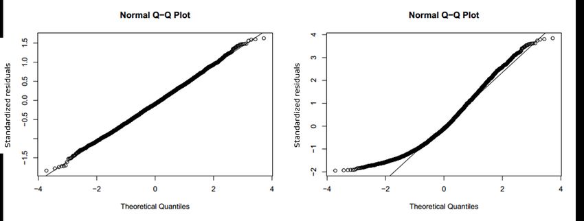
2.4.1 Normality
As mentioned in assumption 6 there is necessity for the residuals to be nor-
mal distributed for confidence intervals and hypothesis testing. One way
to visualize potential normality problems is by using a Normal Quantile
Quantile Plot (Normal Q-Q plot). By presenting the standardized residuals
versus the theoretical quantiles normality problems are visualized by devi-
ations from the straight line. In figure 2 we see a case where normality is
present (left) and where it is not (right). Further, under section Hypothesis
testing a hypothesis test testing for normality in a sample is described.[3]
Figure 2: Normal Q-Q plot
152.4.2 Cook’s Distance
When validating a model, diagnostics of influential points in regards to both
leverage and influence are important. Points with high leverage, points
with an unusual independent variable illustrated by point A in figure 3,
will not affect the value of β̂ but affect statistics such as R2 . Points with
high influence, points with unusual relation between the independent and
dependent variable on the other hand, illustrated by point B in figure 3, will
impact the β̂ as it pulls the model in its direction. [3]
Figure 3: Illustration of points of Leverage and Influence
A concept introduced by Ralph Dennis Cook presented in 1977 is the Cook’s
distance or Cook’s D.[5] Often denoted Di it’s used to detect influential
outliers among predictor variables. By removing the ith data point and
recalculating the regression it illustrates how much the removal affects the
regression model. The formula for Cook’s D is
(ŷ(i) − ŷ)t (ŷ(i) − ŷ)
Di = (7)
pM SRes
and can be rewritten as
ri2 hii
Di = , i = 1, 2, ..., n (8)
p 1 − hii
Hence, disregarding the constant term p, Di depends on the square of the
hii
ith studentized residual and the ratio 1−h ii
, the distance from the predictor
vector xi to the centroid of the remaining data and thus by combining
residual size as well as location in x space Cook’s distance is a suitable
tool for detecting outliers, with values Di > 1 usually considered being
influential. [3]
162.4.3 Hypothesis testing
Hypothesis testing is a procedure testing the plausibility of a hypothesis and
involves the following steps:[6]
1. State the null hypothesis H0 and the alternative hypothesis H1 .
2. Determine the test size, i.e. deciding on one or two tailed and defining
the level of significance α, under which H0 is rejected.
3. Compute the test statistic, appropriately, and derive the distribution.
This step involves the construction of confidence intervals.
4. From 2 and 3 a decision is then made, either rejecting or accepting H0 .
2.4.3.1 Shapiro-Wilk test
A Shapiro-Wilk test tests H0 that a sample x1 , ... ,xn is normally dis-
tributed. The test statistic is
( ni=1 ai x(i) )2
P
W = Pn 2
(9)
i=1 (xi − x̄)
where x(i) is the ith order statistic, i.e. the the ith smallest number in the
sample of x0i s and x̄ is the sample mean. Further ai is given by
t V −1
(ai , · · · , an ) = m C where C is the Euclidean norm C = V −1 m 2 and
the vector m is made of the the expected values of the order statistics of
i.i.d. random variables sampled from the standard normal distribution and
V is the covariance matrix of mentioned normal order statistics.
For a Shapiro-Wilks test H0 is that the sample is normally distributed and
thus if the p-value is less than the chosen significance level α H0 is rejected.[7]
2.4.3.2 F-statistic
By definition SSR (sum of squares regression) = ni=1 (ŷi − ȳ)2 and under the
P
assumption that Var(ε) = σ 2 I, SS
σ2
R
follows χ2 distribution with degrees of
freedom equals to non-centrality parameter λ = σ12 βR t X t X β , where
C C R C
indicates that the matrix X is reduced by removing the columns containing
ones and thereafter centered and R indicates that β is reduced by removing
the intercept β0 .
17Further by definition SSRes (sum of squared residuals) = ni=1 (yi − ŷi )2 and
P
that SSσRes
2 follows χ2 distribution with (n-p) degrees of freedom.
The F statistic is the ratio of two independent χ2 random variables each
divided by their degrees of freedom. As SS σ2
R
and SSσRes
2 are independent
2
under the assumption Var(ε) = σ I the F statistic is formed by
SSR M SR
kσ 2 σ2 M SR
F0 = SSRes
= M SRes
= ∼ Fk,n−p (10)
M SRes
(n−p)σ 2 σ2
and H0 : β1 = β2 = · · · = βk = 0 is rejected if F0 > Fα,k,n-p and the F-test
can be seen as a test of significance of the regression.[3] This result is often
summarized in the ANOVA (analysis-of-variance table) seen in table 1.
Table 1: ANOVA table
Source of Variation Sum of Squares Degrees of Freedom Mean Square F0
Regression SS R k MSR MSR /MSRes
Residual SSRes n-p MSRes
Total SST n-1
For the partial F-statistic referred to under the section Variable selection
the statistic is instead formed by
SSRreduced model −SSRnon−reduced model
∆p
F = ∼ F∆p,n−p (11)
M SResnon−reduced model
where ∆p is the difference in number of regressors and p is the number
of regressors in the non-reduced model and H0 is in this case that the ∆p
regressors under consideration are zero.[8]
2.4.3.3 t-statistic
After F-test completion we have determined that at least one of the re-
gressors are important and the logical next step are questioning which ones.
The hypothesis testing for the significance of individual regressors is the t-
test. The hypothesis are H0 : βj = 0, and H1 : βj 6= 0 and if H0 is rejected
the regressor j stays in the model. The test statistic is defined as
β̂j
t0 = q ∼ tn−p (12)
σ̂ 2 (X t X)−1
jj
q
since SE(βj ) = V ar(βj )= σ 2 (X t X)−1
p 2
jj and can be estimated using σ̂ =
M SRes .[3]
182.4.3.4 Confidence Interval
With the assumptions that the errors εi are i.i.d. normally distributed with
mean zero and variance σ 2 confidence intervals (CI) can be constructed for
the regression coefficients βj,j=0,1,··· ,k . As β ∼ N (β, σ 2 (X t X)−1 ) the t-test
statistic for βj equals
β̂j − βj
t0 = q ∼ tn−p (13)
σ̂ 2 (X t X)−1
jj
where σ̂ 2 = M SRes . Based on (13) a 100(1-α) percent CI for βj is defined
as
q
β̂j ± tα/2,n−p σ̂ 2 (X t X)−1
jj (14)
[3]
2.4.4 Transformation
The basic CLR assumptions 2 and 3 regarding the model errors having mean
zero, constant variance and being uncorrelated can be shown to be violated
during model adequacy checks and thus showing signs of heteroscedasticity.
In this case data transformations may be used as a tool to improve the
homoscedasticity. Both the regressors and the response can be subject to
transformations and data transformations may be chosen heuristically, by
trial-and-error or by analytical procedures.[3]
2.4.4.1 Heuristic approach
By observing the relationship between the response y and one of the re-
gressors xi a pattern may suggest a certain transformation of the regressor.
In figure 4 the pattern suggest the transformation of x’=1/x which linearized
the relationship as seen in figure 5.
19Figure 4: Before transformation Figure 5: After transformation
2.4.4.2 Box-Cox Transformation
An analytical approach is the Box-Cox Transformation which aims to trans-
form the response y using the power transformation y λ where λ is the param-
eter determined by the Box-Cox method. George Box and Sir David Cox
showed how one by the use of maximum likelihood simultaneously could
estimate the regression coefficients and λ.[9]
First, for obivous reasons, problems arise as λ equals zero. Thus the appro-
priate procedure is using
( λ
y −1
, λ 6= 0
y (λ) = λẏλ−1 (15)
ẏ ln(y) , λ = 0
1
where ẏ = ( ni=1 yi ) n is the geometric mean of the observations to fit the
Q
model Y(λ) = Xβ + ε.
The λ found through the maximum-likelihood procedure is the λ for which
the residual sum of squares is minimum, i.e. SSRes (λ) is minimum. Further
an estimate of the confidence interval can be found which could be beneficial
in two cases; primarily if the λ found is for example 1.496 but 1.5 is a part of
the CI one might opt for choosing 1.5 simplifying calculations, and secondly
if λ = 1 is a part of the CI a transformation may not be necessary. Such an
interval consists of the λ that satisfy
1
L(λ̂) − L(λ) ≤ χ2α,1 (16)
2
where λ̂ is the ML estimate.[3]
202.4.5 R2 and RAdj
2
Another way to evaluate model adequacy is by the Coefficient of determi-
nation R2 and is defined as
SSR SSRes
R2 = =1− (17)
SST SST
and is thus often referred to as the proportion of variation explained by the
regression and it follows that 0 ≤ R2 ≤ 1 where 1 indicates that the regres-
sion model explains all variation in the response and vise versa.
However, when comparing and evaluating different models with varying
number of regressors the R2 is biased. Moreover, R2 never decreases as more
regressors are added and thus generally favors models with more regressors
and by solely using R2 one risks adding more variables than necessary and
2
overfitting the model. Therefore the use of RAdj is favored, defined as
2 SSRes /(n − p)
RAdj =1− (18)
SST /(n − 1)
2
Hence, RAdj will only increase if adding variables reduces the residual mean
square (MSRes ) and penalizes adding non-helpful regressors effectively mak-
2
ing RAdj a better tool in comparing competing models of different complexity.[3]
2.4.6 AIC and BIC
The Akaike Information Criterion (AIC) estimates the out-of-sample pre-
diction error and thereby gives the relative quality of the statistic model
given the data. It is defined as follows,
AIC = 2p − 2 ln(L̂) (19)
where p is the number of estimated parameters in the model and L̂ is the
maximum value of the likelihood function for the model. The lower the score,
the better the model is effectively maximizing the expected information.
However, when the sample size is small, the AIC is more likely to overfit,
which the AICc was developed to address. It is defined as follows,
2p2 + 2p
AICc = AIC + (20)
n−p
where n is the sample size. Note that AICc converges to AIC as n → ∞.
21There are also different Bayesian Information Criterion BIC that gives
greater penalties for adding regressors as the sample size increases and one
is the Schwartz criterion and is defined as
BICSch = p ln(n) − 2 ln(L̂) (21)
[3]
2.4.7 Mallow’s Cp
Mallow’s Cp presents a criterion based variance and bias and is defined as
SSRes (p)
Cp = − n + 2p (22)
σ̂ 2
and it can be shown that if the p-term model have zero bias the estimated
value of the Cp equals p. Thus, visualizing different models based on their
Cp as in figure 6 can aid in model selection. For models above the line bias
is present. However, some bias may be accepted in return for a simpler
model and in this case C may be preferred over A although in includes some
bias.[3]
Figure 6: Mallows Cp
222.4.8 VIF
To deal with the problem of multiocollinearity, or rather diagnose a model
based on it’s multicollinearity something called variance inflation factors
(VIF) can be used. The VIF for a regressor indicates the combined effect
of the dependencies among the regressors on the variance of that term.
Hence one or more large VIFs, experience tells us that values exceeding
5-10 are large, indicated presence of multicollinearity and thus a poorly
estimated regression model. Thus comparing VIFs between models as well as
for evaluating a reduced to a non-reduced model is desirable for evaluation.
The VIF is mathematically defined as the diagonal elements of the (X t X)−1
1
matrix when in correlation form, i.e. V IFj = 1−r 2 where 0 ≤ |rj | ≤ 1 and
j
will be close to one, increasing the V IFj , when the regressor j is nearly
linearly dependent on other regressors.[3]
2.4.9 Cross Validation
One method of estimating the prediction error of the model is using cross
validation, a so called resampling method. When cross validation is used
the dataset is divided into two sets; the training set and the testing set. The
model is fitted with the training set and the testing set is used as ”new”
data to estimate the prediction error.
Using repeated k-fold cross validation signifies using k equally large datasets
(divisions of the original observations) which are all used as testing sets in
order for the average prediction error to be calculated. This is repeated m
times with the different divisions of the original dataset and leads to k × m
cross validations per model.[3]
233 Methodology
3.1 Data Collection
The data was collected from the PGA Tour’s website for the years 2004 to
2019.[10] The performance measures of 40 players per year were extracted
resulting in a total of 640 data points.
The data extracted from the website was saved as PDFs, one per player and
season, and Visual Basic was used to via Excel transform them into a R
compatible CSV-file.
3.1.1 Pre-Processing
Firstly our response, season prize money, was corrected according to the
inflation in the US, making it possible to compare data points from different
years. Secondly, after the data extraction was done, there were 102 perfor-
mance measures per data point. By doing a qualitative variable selection,
the number of performance measures shrunk from 102 to 56 and the number
of observations from 640 to 581, reasons for which are further discussed in
discussion section 5.2.
3.1.2 A first look at the data
To get an initial grasp of the predictors that may be included in the final
model all predictors were plotted individually against Official Money and
their correlation were calculated. This heuristic approach pointed to several
promising predictors: long approaches (several different predictors), Greens
In Regulation Percentage and Driving Distance. These predictors all had an
absolute correlation with Official Money in the range 0.4 - 0.6.
24Figure 7: Plot of Greens In Regulation Percentage against Official Money
However, it should be noted that this process in no way measured any form
of multicollinearity. It is thus likely that these initially promising predictors
may not be included in the final model.
3.2 Variable Selection
D. C. Montgomery, E. A. Peck, and G. G. Vining presents a strategy for
variable section and model building which was used in this project. It is
presented as follows:[3]
1. Fit the largest model possible to the data.
2. Perform a thorough analysis of this model.
3. Determine if a transformation of the response or of some of the regres-
sors is necessary.
254. Determine if all possible regressions are feasible.
• If all possible regressions are feasible, perform all possible regres-
sions using suitable criteria to rank the best subset models.
• If all possible regressions are not feasible, use stepwise selection
techniques to generate the largest model such that all possible re-
gressions are feasible. Perform all possible regressions as outlined
above.
5. Compare and contrast the best models recommended by each criterion.
6. Perform a thorough analysis of the ”best” models. Usually 3-5 models.
7. Explore the need of further transformations.
8. Discuss with the subject-matter experts the relative advantages and
disadvantages of the final set of models.
Furthermore, for step 6 in the list above the author suggested the following
sub-steps:[3]
1. Are the usual diagnostic checks for model adequacy satisfactory? For
example, do the residual plots indicate unexplained structure or out-
liers or are there one or more high leverage points that may be con-
trolling the fit? Do these plots suggest other possible transformation
of the response or of some of the regressors?
2. Which equations appear most reasonable? Do the regressors in the
best model make sense in light of the problem environment? Which
models make the most sense from the subject - matter theory?
3. Which models are most usable for the intended purpose? For exam-
ple, a model intended for prediction that contains a regressor that is
unobservable at the time the prediction needs to be made is unusable.
Another example is a model that includes a regressor whose cost of
collecting is prohibitive.
4. Are the regression coefficients reasonable? In particular, are the signs
and magnitudes of the coefficients realistic and the standard errors
relatively small?
5. Is there still a problem with multicollinearity?
263.2.1 Largest possible model and initial transformations
As a first step after collecting and processing the data, a model consist-
ing of all 56 predictors was fitted to the response variable with the built
in R-function lm(). This initial model had a RAdj 2 value of 0.589, worrying
residuals and high VIFs (several over 10 and the highest was Rough Proxim-
ity’s of 122), which hinted that variable selection and some transformations
were in order. Firstly, as discussed earlier in the report, the prize money
on the PGA Tour grows exponentially by ranking, which is why we took
the logarithm of the response Official Money. Secondly, since the number
of events played by a player most likely should be a multiplicative factor
in their total earnings, we also took the logarithm of the predictor Events
Played. Lastly, potential outliers were also identified with measurements
such as Cook’s distance, leverage and residuals. The outliers were removed,
which resulted in a model with RAdj2 = 0.786 and the residuals presented in
figure 8.
Figure 8: Residuals of initial model vs their respective fitted values
The boxcox()-function in the library EnvStats was used to check if any fur-
ther transformation of the response was necessary. As λ = 1 was outside
the confidence interval given by the Box-Cox optimization, a transformation
was performed.
27Figure 9: Log-likelihood graph for the BoxCox parameter λ
with the 95 % confidence interval shown
After the BoxCox transformation the residual for the fitted model looked as
follows:
Figure 10: Residuals of initial model vs their respective fitted
values after BoxCox transformation with λ = 2.57
283.2.2 Stepwise regression
Stepwise regression was performed with the help of the olsrr -function
ols step both p(). The significance level for an entering variable was set to
α = 0.05, and the significance level for en exiting variable to α = 0.01, which
resulted in 20 predictors. Something noteworthy is that the reduced model
did not lose a significant amount of accuracy, the model consisting of 20
2
variables had a RAdj value of 0.748. As 20 is in the interval of the feasible
number of predictors for an all possible regressions analysis (Section 2.3.1)
no further heuristic variable selection was performed.
2
Figure 11: The graphs shows how the RAdj varies with every step of the stepwise regression,
that is either an addition or a removal of a predictor.
293.2.3 All possible regressions
With the predictors selected by the stepwise regression all possible regres-
sions was performed with ols step all possible() from the package olsrr. Since
there was 20 possible predictors to include in the models, 220 = 1, 048, 576
models were tested and ranked by different measures∗ , including AIC, BIC,
2
RAdj and Mallow’s Cp . Since these measures all depend on the mean square
error and penalizes the number of predictors, they all recommend the same
model within the subsets of models with equal numbers of predictors. How-
ever, when comparing models with different numbers of predictors, they do
differ.
In the following graph all the tested models where plotted with the numbers
2
of predictors on the x-axis and their respective RAdj on the y-axis. The red
triangles and the corresponding number represents the best model for every
number of predictors.
Figure 12: The graphs shows the result of the all possible regression where every blue
point represents one model.
2
One clearly sees that the RAdj improves significantly until about 12 pre-
dictors. This also held for the other measurements. This indicated that
choosing a model with less than 12 predictors may jeopardize its accuracy.
∗
This took a little more than 80 hours
30The 10 best models with the number of predictors varying between 11 and
20 were selected for further viewing. These are presented in table 2.
Table 2: Summary of initial models
Model number Number of predictors 2
RAdj AIC Cp
1048575 (I) 20 0.7527425 6944.485 21.00000
1048555 (II) 19 0.7505097 6948.753 25.07500
1048365 (III) 18 0.7480356 6953.531 29.71749
1047225 (IV) 17 0.7452406 6958.984 35.11195
1042380 (V) 16 0.7423691 6964.539 40.70396
1026876 (VI) 15 0.7365307 6976.610 53.11051
988116 (VII) 14 0.7301641 6989.534 66.77582
910596 (VIII) 13 0.7244185 7000.821 79.06578
784626 (IX) 12 0.7164660 7016.402 96.48104
616666 (X) 11 0.6999963 7048.286 133.5952
2
As said above, the RAdj seems to be quite stable as the number of predic-
tors decrease from 20 to 12 variables. However, when the model is reduced
2
further the decrease in RAdj seems to accelerate, indicating that the model
shouldn’t be reduced to fewer than 12 predictors. In contrast, all models
seem to be biased according to Mallow’s Cp and the bias increases quickly
for every predictor removed. This indicates that the model shouldn’t be
reduced too much.
Looking at all the measurements and simultaneously trying to keep the size
of the models down for simplicity’s sake, we chose to continue with model
III-VIII for a further analysis.
313.3 Promising Models
Table 3: Predictors included in the chosen models
Predictor III IV V VI VII VIII
Sand Save Percentage X X X X X X
Approaches From > 200 Yards X X X X X X
Average Distance Of Putts Made X X X X X X
Events Played X X X X X X
Driving Distance X X X X X X
Scrambling From 10 - 20 Yards X X X X X
Approaches From 175 - 200 Yards X X X X X X
Scrambling From > 30 Yards X X X X X X
Driving Accuracy Percentage X X X X X X
Approaches From 50 - 125 Yards X X X X X X
Fairway Proximity X X X X X X
Approaches From 150 - 175 Yards X X X X X X
Approaches From 125 - 150 Yards X X X X X X
Putting - Inside 10’ X X X X X X
Approaches From > 275 Yards X X X X
Putting From 7’ X X X
Scrambling From < 10 Yards X X
Longest Putts X
Approaches From > 200 Yards (Rough)
Approaches From 50 - 75 Yards
The six models chosen in the previous section are summarized in table 3,
which shows which of the 20 variables selected by the stepwise regression
are included in the respective models.
323.3.1 Model Validation
All six models did not seem to have any major problem regarding residuals
or influential points. There was no obvious heteroscedasticity (see figure 24)
and the point with the highest potential of being an influential point had
a Cook’s distance of below 0.08 (see figure 26). In addition, the Q-Q plots
did not show any glaring evidence of the residuals differing from a normal
distribution (see figure 25).
3.3.2 Variable Selection
Looking at reasonability of the included predictors from a golfing perspective
and their respective estimated coefficients magnitude and signs we concluded
that Longest Putts, Putting From 7’, Approaches From > 275 Yards, and
Fairway Proximity should be excluded from the final model. Further, look-
ing at the remaining predictors respective significance, we concluded that
we should choose a model where the variables Scrambling From < 10 Yards,
Longest Putts and Approaches From > 200 Yards (Rough) are not included.
The reason for this will be discussed further in section 5.4.
3.3.3 Multicollinearity
When taking a look at the variance inflation factors of the predictors one
could see that all but one of them falls in to the range 1 - 3. Fairway Prox-
imity, however, has a VIF of around 7, depending on which model the VIFs
are calculated for, indicating that it correlates with at least one of the other
predictors.
The bar plots of model III:s and VIII:s VIFs are shown in Figure 13 and
14 respectively. Firstly, one sees that Fairway Proximity:s bar sticks out
from the rest. Secondly, one also sees that the VIF:s of model VIII are
slightly smaller than those of model III:s since there should be less overall
correlation when there are fewer predictors included in the model. This,
together with the points discussed in the previous section made us chose
model VII with Fairway Proximity removed as the final model. This will be
further discussed in section 5.4.
33Figure 13: VIFs of model III Figure 14: VIFs of model VIII
3.3.4 Possible transformations
Once again we looked for necessary transformations of the response (now
on the final model) by using the Box-Cox transformation. The suggested
exponent was 1.16 and one clearly sees in Figure 15 that λ = 1 lies within
the 95% CI.
Figure 15: Log-likelihood graph for the BoxCox parameter λ with the 95 %
confidence interval shown.
This indicates that no further transformation of the response variable is nec-
essary and the lambda for the final model remains being 2.57.
343.3.5 Cross Validation
Repeated five-fold cross validation was performed on model V with 10 rep-
etitions. The average RAdj2 , R̄2
Adj = 0.6695, of the models based on the
re-sampled dataset did not differ significantly from the value without any
2
re-sampling, RAdj = 0.6918, indicating a good fit. In addition, the root-
mean-square-error and the mean-absolute-error were quite small in compar-
ison to the average response-value, namely 11.37% and 8.95% respectively.
354 Results
4.1 Final Model
The final model consists of 13 predictors and an intercept. Its regression
equation is described in equation (23) below where y is the response Official
Money.
(ln(y))2.57 = − 3905.0545
+ 441.1038 · xSandSaveP ercentage
− 26.7400 · xApproachesF rom>200Y ards
+ 21.5155 · xAverageDistanceOf P uttsM ade
+ 151.2015 · ln(xEventsP layed )
+ 8.9043 · xDrivingDistance
+ 429.1561 · xScramblingF rom10−20Y ards
− 36.8731 · xApproachesF rom175−200Y ards (23)
+ 302.4759 · xScramblingF rom>30Y ards
+ 759.1370 · xDrivingAccuracyP ercentage
− 40.2363 · xApproachesF rom50−125Y ards
− 26.9964 · xApproachesF rom150−175Y ards
− 22.7777 · xApproachesF rom125−150Y ards
+ 1858.3662 · xP utting−Inside100
This can be rewritten as,
13
X 1
y = exp((βˆ0 + β̂i xi ) λ ) (24)
i=1
where the indices represent that names of the predictors in equation (23),
β̂i their coefficients and λ = 2.57.
In the following table, Table 4, the 13 predictors in the final model and its
intercept are summarized.
36Table 4: Summary of coefficients in the final model Predictor [j] β̂j Std. Error p-value (Intercept) -3,905.0545 394.8379 200 Yards -26.7400 4.8073 4.10e-08 Average Distance Of Putts Made 21.5155 3.5099 1.65e-09 Events Played 151.2015 12.8785
4.2 Impact of Performance Measures
With these results we will now try to answer the original question: Which
performance measures drive PGA Tour prize money?
This was done by improving the performance measures one by one with a
percentage of their respective standard deviation (of all data points). How-
ever, for the performance measure Events Played we will add one additional
event. An explanation of why this method was chosen can be found in sec-
tion 5.4.
We will look at two different players, Tiger Woods 2005 (his best year in prize
money earned adjusted to inflation) and Joe Meanson (a fictional player that
is average in every performance measure).
Table 6: A summary of the standard deviations of the predictors in the final model and
the performance measures of the two players that will be looked in to. Official Money is
calculated with equation (24).
Predictor σ Tiger Woods Joe Meanson
Sand Save Percentage [%] 0.0626 0.54 0.50
Approaches From > 200 Yards [m] 1.156 14.45 15.34
Average Distance Of Putts Made [m] 1.321 24.64 22.50
Events Played 5.975 20 22.61
Driving Distance [yds] 9.578 316.1 291.74
Scrambling From 10 - 20 Yards [%] 0.0503 0.70 0.65
Approaches From 175 - 200 Yards [m] 0.724 8.33 10.10
Scrambling From > 30 Yards [%] 0.0654 0.29 0.29
Driving Accuracy Percentage [%] 0.0530 0.55 0.62
Approaches From 50 - 125 Yards [m] 0.499 5.03 5.67
Approaches From 150 - 175 Yards [m] 0.601 8.15 8.41
Approaches From 125 - 150 Yards [m] 0.559 6.05 6.98
Putting - Inside 10’ [%] 0.0134 0.89 0.87
Official Money [$] 14,038,107 1,588,413
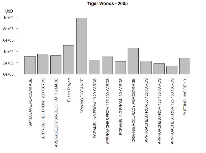
384.2.1 Example: Tiger Woods
Following is a table (Table 7) showing Tiger Woods expected increase in
prize money earned over the 2005 season if one of the performance measures
in the final model would be improved by a multiple of its standard deviation.
Table 7: How much Tiger Woods prize money would increase if one of his performance
measures would increase by a factor times the standard deviation of that performance
measures. 3 significant digits.
Predictor σj 0.167σj 0.01σj
Sand Save Percentage 1,970,000 (+14.0%) 314,000 (+2.2%) 18,600 (+0.13%)
Approaches From > 200 Yards 2,220,000 (+15.8%) 352,000 (+2.5%) 20,800 (+0.15%)
Average Distance Of Putts Made 2,030,000 (+14.5%) 323,000 (+2.3%) 19,100 (+0.14%)
Events Played 504,000 (+3.6%)
Driving Distance 6,920,000 (+49.3%) 990,000 (+7.1%) 57,500 (+0.41%)
Scrambling From 10 - 20 Yards 1,520,000 (+10.8%) 245,000 (+1.7%) 14,500 (+0.10%)
Approaches From 175 - 200 Yards 1,900,000 (+13.6%) 304,000 (+2.2%) 18,000 (+0.13%)
Scrambling From > 30 Yards 1,390,000 (+9.9%) 224,000 (+1.6%) 13,300 (+0.09%)
Driving Accuracy Percentage 2,960,000 (+21.1%) 460,000 (+3.3%) 27,100 (+0.19%)
Approaches From 50 - 125 Yards 1,410,000 (+10.1%) 228,000 (+1.6%) 13,500 (+0.10%)
Approaches From 150 - 175 Yards 1,130,000 (+8.1%) 184,000 (+1.3%) 10,900 (+0.08%)
Approaches From 125 - 150 Yards 880,000 (+6.3%) 144,000 (+1.0%) 8,560 (+0.06%)
Putting - Inside 10’ 1,760,000 (+12.6%) 282,000 (+2.0%) 16,700 (+0.12%)
39The case where the improvement of the performance measures is 0.167σj is
shown in the bar plot in Figure 16.
Figure 16: How much Tiger Woods prize money would increase if one particular perfor-
mance measure would improve by 0.167σj (which is equal to 1 for Events Played to 3
significant digits).
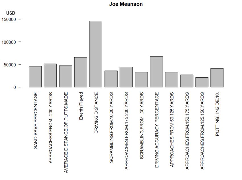
404.2.2 Example: Joe Meanson
Following is a table (Table 8) showing Joe Meansons expected increase in
prize money earned over a season if one of the performance measures in the
final model would be improved by a multiple of its standard deviation.
Table 8: How much Joe Meanson prize money would increase if one of his performance
measures would increase by a factor times the standard deviation of that performance
measures. 3 significant digits.
Predictor σj 0.167σj 0.01σj
Sand Save Percentage 292,000 (+17.7%) 46,000 (+2.8%) 2,720 (+0.16%)
Approaches From > 200 Yards 330,000 (+20.0%) 51,600 (+3.1%) 3,040 (+0.18%)
Average Distance Of Putts Made 302,000 (+18.3%) 47,400 (+2.9%) 2,800 (+0.17%)
Events Played 65,500 (+4.0%)
Driving Distance 1,060,000 (+64.0%) 146,000 (+8.8%) 8,410 (+0.51%)
Scrambling From 10 - 20 Yards 225,000 (+13.6%) 35,900 (+2.2%) 2,130 (+0.13%)
Approaches From 175 - 200 Yards 282,000 (+17.1%) 44,500 (+2.7%) 2,630 (+0.16%)
Scrambling From > 30 Yards 205,000 (+12.4%) 32,900 (+2.0%) 1,950 (+0.12%)
Driving Accuracy Percentage 441,000 (+26.7%) 67,500 (+4.1%) 3,970 (+0.24%)
Approaches From 50 - 125 Yards 208,000 (+12.6%) 33,400 (+2.0%) 1,980 (+0.12%)
Approaches From 150 - 175 Yards 167,000 (+10.1%) 26,900 (+1.6%) 1,600 (+0.10%)
Approaches From 125 - 150 Yards 130,000 (+7.9%) 21,100 (+1.3%) 1,250 (+0.08%)
Putting - Inside 10’ 261,000 (+15.8%) 41,400 (+2.5%) 2,450 (+0.15%)
41The case where the improvement of the performance measures is 0.167σj is
shown in the bar plot in Figure 17.
Figure 17: How much Joe Meanson prize money would increase if one particular perfor-
mance measure would improve by 0.167σj (which is equal to 1 for Events Played ).
425 Analysis & Discussion
5.1 Analysis of Final Model
The final model consists of 13 variables, which are summarized in table 9.
Table 9: Predictors included in the final model.
Driving... Approaches From... Short Game Miscellaneous
Distance 50 - 125 Yards Sand Save Percentage Events Played
Accuracy Percentage 125 - 150 Yards Scrambling From 10 - 20 Yards
150 - 175 Yards Scrambling From > 30 Yards
175 - 200 Yards Putting - Inside 10’
> 200 Yards Average Distance Of Putts Made
When one is only looking at this table one could conclude that approaching
and short game are the most important categories in golf for the PGA Tour
players since they together make up 10 of the 13 predictors in the model.
However, according to to Figure 16 and 17 it seems to be the opposite since
Driving Distance, Events Played and Driving Accuracy Percentage are ex-
pected to have the largest impact on the players income. This may be since
approaching and short game is divided into more performance measures than
other parts of golf, thus making e.g. driving predictors more comprehensive.
This may indicate that an improvement of one standard deviation in one of
the driving predictors compared to one of the approaching predictors is a
much greater actual improvement.
Furthermore, generally approach-shots that are hit from a shorter distance
should end up closer to the hole. If then all approaches (regardless of dis-
tance) had an equal impact on prize money their respective estimated coeffi-
cients should be decreasing in absolute value as the distance increases. This
wasn’t the case; sorted by absolute value of their respective coefficient from
largest to smallest the approach-predictors come in the order 50 - 125, 150
- 175, > 200 and 125 - 150. This indicates that the respective approach-
predictors don’t have an equivalent impact on the response variable Official
Money, which is backed by Table 7 and 8 where Approaches From > 200
Yards was shown to have the largest impact.
One interesting analysis would be if according to the final model, if an in-
crease (+1) in Events Played would lead to a linear increase in expected
prize money equivalent to the current average prize money per event. Look-
ing at the players discussed in section 4.2 we see that Tiger Woods expected
43earnings per event was $702,000 and his expected earnings for playing one
more event was $504,000. On the contrary, Joe Meanson’s expected earnings
per event was $70,300 and his expected earnings for playing one more event
would was $65,500. This may indicate the additional events one adds to ones
schedule may not be as profitable as the previous, maybe because players
tend to choose events that they are expected to earn a lot at first. These
events may have a large prize pool or they may fit that specific player’s
playstyle. This analysis was made possible by us not using Official Money
Per Event as the response, since it enabled us to use Events Played as a
predictor.
Another interesting observation is that no approaching-from-the-rough or
left/right-tendency predictors survived to the final model. This probably in-
dicates that they aren’t good at predicting prize money since the predictors
of the final model were chosen by looking at their relevance, reasonability,
significance level and effect on multicollinearity. However, it is not impossi-
ble that they do have an impact on prize money, but it is not big enough to
detect in the shadow of the other predictors.
While on the topic of predictors that were excluded from the final model the
careful reader will notice that Greens In Regulation Percentage is missing
from the final model even though it was deemed promising in Section 3.1.2.
This particular predictor was removed during the stepwise regression at step
12, when the model consisted of 11 variables, as one can see in Figure 11.
It was probably removed due to it having multicollinearity with short game
and approaching predictors. Since it was removed before the model reached
the size of the final model, we are fairly confident that too much precision
wasn’t lost from it not being part of the all possible regression.
Lastly the intercept is seemingly quite large in absolute terms in relation
to the other coefficients, calculated to −3, 905 compared to second largest
being β̂P utting−Inside100 = 1, 858. One might from equation (24) expect a
large negative intercept and that this indicates that Official Money would
be close to 0 as the other predictors are set to 0. However, one have then
failed to account for the exponent λ1 which due to being less than 1 (λ = 2.57)
implies that βˆ0 + 13
P P13
i=1 β̂i xi must be larger than 0 and the sum i=1 β̂i xi
to be larger than 3, 905 to produce a real answer. This enables a player’s
performance measure to not yield a positive return, expectedly as players
will not win prize money regardless of their performance measures.
445.2 Data Pre-Processing
We started of with 102 predictors and 640 data points, however several data
points were incomplete and some of the performance measures were only
measured for a small group of players. Thus, performance measures for
which a lot of data points had missing were removed and incomplete data
points too. Performance measures that directly affected score (such as Av-
erage Score and Birdie Average) were also removed as they can’t indicate
a specific part of the players game they can improve. Furthermore, we also
chose to exclude all Strokes Gained performance measures since we wanted
more precise predictors, e.g. Strokes Gained Approach-The-Green and -
Putting is a combination of all approach-the-green and putting predictors
respectively. All these measures shrunk the number of predictors to 56 and
data points to 581.
While the PGA Tour website provided an abundance of data points and pre-
dictors it was very labour-intensive to extract. It had to be done manually
and took about one minute per data point, which stopped us from collecting
more data than may have been necessary. We do however think that the
around 600 data points were enough to perform a solid analysis.
5.3 Handling of Outliers
Five data points in the data set were deemed to be outliers since they had
large residuals, Cook’s distances and deviances in the Q-Q plot. These
were the data points 11, 128, 326, 415 and 585 which are evenly distributed
between 1 and 640 indicating that there is no trend regarding outliers and
year (the data set is sorted by year). They did however have a noticeable
effect on the precision of the model; the first model consisting of all 56
variables increased its adjusted R2 value by 0.0113, from 0.7749 to 0.7862.
45You can also read