Seasonal biological carryover dominates northern vegetation growth - Boston University
←
→
Page content transcription
If your browser does not render page correctly, please read the page content below
ARTICLE
                  https://doi.org/10.1038/s41467-021-21223-2                 OPEN

                  Seasonal biological carryover dominates northern
                  vegetation growth
                  Xu Lian 1, Shilong Piao 1,2,3 ✉, Anping Chen 4, Kai Wang 1, Xiangyi Li                                           1,   Wolfgang Buermann5,6,
                  Chris Huntingford 7, Josep Peñuelas 8,9, Hao Xu1 & Ranga B. Myneni10
1234567890():,;

                  The state of ecosystems is influenced strongly by their past, and describing this carryover
                  effect is important to accurately forecast their future behaviors. However, the strength and
                  persistence of this carryover effect on ecosystem dynamics in comparison to that of
                  simultaneous environmental drivers are still poorly understood. Here, we show that vege-
                  tation growth carryover (VGC), defined as the effect of present states of vegetation on
                  subsequent growth, exerts strong positive impacts on seasonal vegetation growth over the
                  Northern Hemisphere. In particular, this VGC of early growing-season vegetation growth is
                  even stronger than past and co-occurring climate on determining peak-to-late season
                  vegetation growth, and is the primary contributor to the recently observed annual greening
                  trend. The effect of seasonal VGC persists into the subsequent year but not further. Current
                  process-based ecosystem models greatly underestimate the VGC effect, and may therefore
                  underestimate the CO2 sequestration potential of northern vegetation under future warming.

                  1 Sino-French Institute for Earth System Science, College of Urban and Environmental Sciences, Peking University, Beijing, China. 2 Key Laboratory of Alpine

                  Ecology, Institute of Tibetan Plateau Research, Chinese Academy of Sciences, Beijing, China. 3 Center for Excellence in Tibetan Earth Science, Chinese
                  Academy of Sciences, Beijing, China. 4 Department of Biology and Graduate Degree Program in Ecology, Colorado State University, Fort Collins, CO, USA.
                  5 Institute of Geography, Augsburg University, Augsburg, Germany. 6 Institute of the Environment and Sustainability, University of California, Los Angeles, Los

                  Angeles, CA, USA. 7 UK Centre for Ecology and Hydrology, Wallingford, Oxfordshire, UK. 8 CREAF, Cerdanyola del Valles, Barcelona, Catalonia, Spain. 9 CSIC,
                  Global Ecology Unit CREAF-CSIC-UAB, Bellaterra, Barcelona, Catalonia, Spain. 10 Department of Earth and Environment, Boston University, Boston, MA, USA.
                  ✉email: slpiao@pku.edu.cn

                  NATURE COMMUNICATIONS | (2021)12:983 | https://doi.org/10.1038/s41467-021-21223-2 | www.nature.com/naturecommunications                                      1
ARTICLE NATURE COMMUNICATIONS | https://doi.org/10.1038/s41467-021-21223-2
B
iological cycles include many successional growth periods in vegetation growth. To test this hypothesis, we quantify the impact
which the past and the present are tightly connected. In such of VGC on NH vegetation growth with a large set of measure-
temporally connected dynamical systems, transient carryover ments, including satellite, eddy covariance (EC), and tree-ring
of the near past is commonly observed for many state variables1–3. chronologies, and compare the size of this effect against that of
The carryover effect of biological states has been extensively immediate and lagged impacts of climate change (see “Methods”).
documented in biomedical research, for example, describing the Our work provides quantitative evidence that peak-to-late season
phenomenon where the effects of medical treatments can carry over vegetation productivity and greenness are primarily determined
from one to another in repeated clinical experiments4. This biolo- by a successful start of the growing season (via the interseasonal
gical carryover effect is also widely existent in plant science2,4–6. The VGC effect), rather than by a transient or lagged response to
life-cycle continuity of plant growth implies that present states of climate. This carryover of seasonal vegetation productivity also
vegetation growth may intrinsically affect subsequent growths, contributes to annual vegetation growth across consecutive years.
which is a type of biological memory2,7, and can be referred to as
vegetation-growth carryover (VGC). The VGC effect could poten-
tially control the pattern of seasonal-to-interannual variations of Results and discussion
vegetation growth. For example, a tree may maintain a greening Interseasonal VGC dominates peak-to-late-season growth. We
signal by cumulatively enhancing carbon uptake8, resulting in extra first examined the VGC effect at the seasonal scale, using satellite-
storage of photosynthate and more substantial leaves and roots. derived Normalized Difference Vegetation Index (NDVI, see
Such structural change of plants may then boost their resistance to “Methods”) for the 1982–2016 period. We defined the dormancy
climate fluctuations9 and emerging disturbances10, unless increas- season (DS) and three periods of the growing season, i.e., EGS,
ing water and heat stress exceeds the tolerance of sustainable tree peak growing season (PGS), and late growing season (LGS), based
growth11. The critical question is thus how strong this VGC effect on phenological metrics (see “Methods”). The partial auto-
is, particularly when compared against concurrently changing correlation calculated for NDVI time series of two consecutive
environmental conditions that also influence the present state of seasons, after factoring out concurrent and preceding climatic
vegetation growth. impacts, provides an estimate of the interseasonal VGC effects
Projections of future vegetation and carbon uptake changes, (see “Methods”). At the hemispheric scale, our analyses show a
including ecosystem capacity to offset CO2 emissions, are highly significant (p < 0.05) control of the NDVI of the preceding season
uncertain12,13, primarily due to our limited understanding of the (NDVIps) on the interannual variations of seasonal NDVI for all
mechanisms that govern vegetation growth dynamics. Surprisingly, three active growing seasons (Fig. 1a). This VGC effect is also
while the concept of vegetation carryover effect is not new, and consistently positive across the majority (79%, 89%, and 94% for
some key analyses searching for evidence of the VGC effect do exist, EGS, PGS, and LGS, respectively) of northern vegetated areas
they are often focused on the short-term carryover14 or limited in (Supplementary Fig. 1). Although the EGS NDVI is more strongly
their spatial scope15. Over a broad geographical range, it remains correlated with EGS temperature, the PGS and LGS NDVIs are
unclear how substantial the role of the VGC effect is in contributing most strongly correlated with NDVIps, rather than climate dri-
to current and future vegetation growth and carbon cycle, parti- vers (Fig. 1a). This VGC is particularly important for under-
cularly in comparison to that of abiotic factors (such as immediate standing vegetation growth in LGS, when climate is known to
and lagged impacts of climate). Indeed, the regulation of vegetation have a weak explanatory power30,31.
growth by abiotic factors, particularly climate and associated epi- The primary role of NDVIps in driving subsequent PGS and LGS
sodic climate extremes, has been extensively investigated and fairly NDVI variations is reaffirmed by conducting partial correlations with
well understood16–22. It is generally accepted that climate variation detrended anomalies of all variables (Supplementary Fig. 2), implying
is the primary driver of seasonal-to-interannual dynamics of vege- a robust coupling of seasonal vegetation growth within a specific
tation growth and associated carbon uptake over the Northern calendar year. Furthermore, the robustness of the satellite-identified
Hemisphere (NH)16–18. Importantly, climate change in the early positive VGC effect dominating vegetation growth in PGS and LGS is
growing season (EGS) may substantially influence vegetation also verified by examining other satellite-derived vegetation growth
growth of late seasons through, for instance, modulating plant proxies, including leaf area index (LAI) and gross primary
transpiration19,23–26 and snow melting27,28, both leading to changes productivity (GPP) (see “Methods”; results in Supplementary Fig. 3).
in soil moisture that can propagate into late seasons25. This climatic Meanwhile, we also noticed some difference between GPP- and
legacy effect via complex vegetation–soil–climate interactions has NDVI-derived LGS-to-EGS VGC effect in some mid-to-high
been now included in many state-of-the-art terrestrial biosphere northern latitudes (Supplementary Fig. 4d). Negative LGS-to-EGS
models29. Still, these models produce a wide divergence in the VGC effect has been found over eastern U.S., North China, and
estimates of vegetation growth and carbon uptake12,13, suggesting western and central Russia based on the GPP dataset (Supplementary
that some related mechanisms are either missing or incorrectly Fig. 4d), suggesting greater uncertainties in LGS-to-EGS VGC effect
parameterized. than EGS-to-PGS and PGS-to-LGS VGC effects.
The interseasonal connections of vegetation growth has In contrast to the consistently strong and positive VGC impact,
received increasing attention in recent years. The legacy the strength and direction of climatic factors in determining the
effect of EGS vegetation growth on mid-to-late-season growth interannual variation of seasonal NDVI, including their immedi-
through transpiration-regulated soil moisture changes19,23,25,26 ate and lagged impacts16–20, is highly variable between seasons
can be categorized as an exogenous memory effect under the and across regions (Fig. 1a and Supplementary Figs. 5 and 6). At
theoretical framework of ecological memory by Ogle et al.2. the hemispheric scale, concurrent seasonal temperature is a
Different from the legacy effect of climate anomalies or the primary and positive factor controlling the interannual variation
exogenous memory of vegetation growth, the VGC effect in this of EGS NDVI during the last 35 years (partial correlation, rp =
work emphasizes how the carryover of the early vegetation 0.83, p < 0.01). The dominance of EGS temperature on EGS
structure may contribute to vegetation growth of the following vegetation growth is also consistently observed when analyzing
seasons, or an endogenous memory effect according to the other satellite-based vegetation proxies of LAI and GPP
framework of Ogle et al.2. (Supplementary Fig. 4). However, temperature has a much
In this study, we hypothesize that the VGC has played a critical weaker impact during PGS (rp = 0.42, p < 0.05) and LGS (rp =
role in regulating the seasonal-to-interannual trajectory of 0.12, p > 0.05) (Fig. 1a). Although higher concurrent temperature
2 NATURE COMMUNICATIONS | (2021)12:983 | https://doi.org/10.1038/s41467-021-21223-2 | www.nature.com/naturecommunicationsNATURE COMMUNICATIONS | https://doi.org/10.1038/s41467-021-21223-2 ARTICLE
a b
0.8 1.5
Immediate climatic effects
0.6
EGS NDVI 1.2 Lagged climatic effects
NDVI trend ( 10-3 yr-1 )
0.4 VGC
Residuals
0.2 0.9
PGS NDVI 0
0.6
-0.2
-0.4 0.3
LGS NDVI
-0.6
0
-0.8
NDVIps TMP ps PREps TMP PRE EGS PGS LGS
Fig. 1 Satellite-based vegetation growth carryover versus climatic effects. a Partial correlation coefficients between 35-year seasonal Normalized
Difference Vegetation Index (NDVI) time series and concurrent climatic factors (temperature, TMP and precipitation, PRE), and climatic factors (TMPps
and PREps) and NDVI (NDVIps) of the preceding season. The subscript ps denotes values for the immediately preceding season, except that ps for early
growing-season (EGS) NDVI refers to NDVI of the preceding late growing season (LGS). Squares with black outline show statistically significant
correlations at the 95% confidence level. b Individual contributions of the vegetation growth carryover (VGC) effect and the immediate and lagged climatic
effects to seasonal NDVI trends over the 35 years (1982–2016) (see “Methods”). The gray dashed line indicates the observed trend of the growing-season
mean NDVI over the Northern Hemisphere, and the gray stars indicate the observed NDVI trend of each season.
generally stimulates vegetation activity in EGS across most of the that the higher peak growth rate in PGS is primarily inherited from
northern vegetated areas (Supplementary Fig. 5a), it has emerged greening of the preceding EGS (48%) rather than from direct
as a limit to PGS and LGS vegetation growth for most of the contributions of PGS climate change (20%) (Fig. 1b).
warm mid-latitudes and some of the high latitudes (Supplemen- Considering the substantial fraction of unexplained variance of
tary Fig. 5b, c). Additionally, temperature also has a negative observed vegetation growth in PGS and LGS after accounting for
legacy effect on vegetation growth in the subsequent season the climate and VGC effect of the concurrent and immediate
(Fig. 1a), most significantly for the DS-to-EGS legacy effect (rp = precedent seasons (residuals in Fig. 1b), we further investigated the
−0.42, p < 0.05). This adverse legacy effect of DS temperature is residual changes of PGS and LGS NDVI with vegetation and
likely due to the lower chilling accumulation required for leaf climatic factors in the previous year (see “Methods”). At the
unfolding in EGS caused by DS warming32. For precipitation, we hemispheric scale, about 58% of the residuals of PGS NDVI
find very weak and statistically insignificant immediate and changes can be explained by all the factors collectively (Supple-
lagged impacts on vegetation growth for all the seasons at the mentary Fig. 7c). NDVI of the previous LGS significantly correlates
hemispheric scale (Fig. 1a). This weak precipitation impact is to PGS NDVI residuals (rp = 0.55, p < 0.05), and contributes the
likely due to a spatial cancelling-out of the positive effects at the most to the variance of residuals (Supplementary Fig. 7a). Among
water-limited mid-latitudes by the negative effects at high the climatic factors, PGS precipitation of the previous year shows
latitudes (more precipitation is often concurrent with increased the strongest correlation (rp = 0.31, p = 0.09) with PGS NDVI
cloudiness and reduced solar radiation reaching vegetation residuals (Supplementary Fig. S7a), indicating a strong legacy effect
canopies) (Supplementary Figs. 5d–f and 6d–f). of precipitation anomalies (such as droughts) on PGS vegetation
For each season, we further derived the individual contributions growth. None of the considered factors shows a significant (p >
of VGC, as well as the immediate and lagged climatic effects, to the 0.05) correlation with LGS NDVI residuals, and collectively they
35-year NDVI trends (see “Methods”). The effects of temperature explain about 20% of LGS NDVI variance (Supplementary
and precipitation were here combined as a single variable of Fig. S7c).
climatic effects. As expected, the strong observed EGS greening We further examined the VGC effect and vegetation–climate
trend (0.0012 yr−1, p < 0.05) is predominately attributed to the connections with seasonal GPP data from the global FLUXNET
concurrent climate change (77%), particularly EGS warming that EC network. The short temporal coverage of EC records prevents
stimulates earlier phenology, followed by smaller but non-negligible calculating temporal correlations, we hence analyzed the
contributions from climate (8%) in the preceding DS and vegetation relationship between the trend of GPP and that of its potential
growth in the preceding LGS (17%) (Fig. 1b). However, for PGS drivers across 50 available flux-tower sites (“Methods”). Con-
and LGS, about half of the observed greening trends (48% and 54%, sistent with the satellite-based findings, we discovered strong
respectively) are attributed to greening in the preceding season, positive cross-site correlations between the trend of GPP and
supporting the notion of a strong positive biological carryover that of its preceding values for all the growing seasons (Pearson
between seasons. In comparison, climate, including its immediate correlation, r = 0.42, 0.70, and 0.82 for EGS, PGS, and LGS,
and lagged effects, plays a much smaller role in PGS and LGS respectively, p < 0.01 in all cases; Fig. 2a). However, temperature
greening (EGS climate may even cause a negative lagged impact on and precipitation changes cannot account for the cross-site
the PGS greening trend; Fig. 1b). Hence, warming-induced greening variation of GPP trends for any season (Supplementary Fig. 8),
in EGS persists into the mid-to-late growing season, and has been even though EGS temperature is identified as the primary driver
the primary source for the overall satellite-observed NH growing- of satellite-based EGS NDVI changes (Fig. 1a). The weak cross-
season greening over the last few decades33,34. It is interesting to site correlation with climatic variables may be overshadowed by
note that PGS is the season whose interannual productivity the biome-dependent sensitivity of GPP to climate16,17. To test
variations most strongly correlate with that of the growing-season this, we examined the cross-site relationship between the GPP
mean35, and trend of vegetation growth most similar to that of the trend and its climatic sensitivities (“Methods”). We found a
growing-season mean (Fig. 1b). However, our results demonstrate significant positive correlation between the EGS GPP trend and
NATURE COMMUNICATIONS | (2021)12:983 | https://doi.org/10.1038/s41467-021-21223-2 | www.nature.com/naturecommunications 3ARTICLE NATURE COMMUNICATIONS | https://doi.org/10.1038/s41467-021-21223-2
a b
0.8 0.8
EGS: r = 0.42, p < 0.01 EGS: r = 0.29, p < 0.05
0.6 0.6
GPP trend (gC m -2 d-1 yr-1 )
GPP trend (gC m -2 d-1 yr-1 )
PGS: r = 0.7, p < 0.01 PGS: r = 0.29, p < 0.05
LGS: r = 0.82, p < 0.01 LGS: r = -0.03, p = 0.85
0.4 0.4
0.2 0.2
0 0
-0.2 -0.2
-0.4 -0.4
-0.6 -0.6
-0.6 -0.3 0 0.3 0.6 -1 -0.6 -0.2 0.2 0.6 1
-2 -1 -1
GPP ps trend (gC m d yr ) Sensitivity of GPP to TMP (gC m -2 d-1 o C -1 )
c d
0.8 1
EGS: r = 0.2, p = 0.16 0.8
0.6
GPP trend (gC m -2 d-1 yr-1 )
PGS: r = -0.04, p = 0.76
0.6
LGS: r = 0.01, p = 0.92
Partial correlations
0.4 0.4 GPP ps
0.2 TMP ps
0.2
0 PREps
0 -0.2 TMP
-0.2 -0.4 PRE
-0.6
-0.4
-0.8
-0.6 -1
-0.6 -0.3 0 0.3 0.6 EGS PGS LGS
Sensitivity of GPP to PRE (gC m -2 mm-1 )
Fig. 2 Site-based vegetation growth carryover versus climatic effects. a Scatterplot of the gross primary productivity (GPP) trend for each season against
that of the preceding season across 50 FLUXNET sites. b Scatterplot of the GPP trend for each season against the GPP sensitivity to concurrent
temperature across 50 FLUXNET sites. c Scatterplot of the GPP trend for each season against the GPP sensitivity to concurrent precipitation across 50
FLUXNET sites. In all panels, best-fitting straight lines are shown for significant relationships, along with related statistics as annotated. d Partial correlation
coefficients between anomalies of seasonal GPP changes and that of each driving factor, based on measurements from 11 Ameriflux sites. Boxplots show
the maximum, upper-quartile, median, lower-quartile, and minimum of the distribution across sites. EGS, PGS, and LGS represent early, peak, and late
growing season, respectively.
its sensitivity to temperature (r = 0.29, p < 0.05) (Fig. 2b), biome differences by grouping northern vegetation into three
supporting that EGS warming controls EGS greening patterns. main vegetation types of temperate grassland, forest, and arctic
For all the other cases, the insignificant (p > 0.05) relationship tundra and shrubland, based on satellite-derived land-cover
between the GPP trend and its climatic sensitivity (Fig. 2b, c) maps (“Methods”; Supplementary Fig. 9). Figure 3 shows all
supports a weak climatic impact. pathways of the EGS–PGS connection (for other interseasonal
In addition to these global datasets, we also used long-term linkages see Supplementary Fig. 10). The SEM analysis
GPP measurements from 11 AmeriFlux EC sites (“Methods”) to identifies the significant positive influence of EGS vegetation
characterize temporal relationships between vegetation growth growth on that of PGS, explaining the largest fraction of PGS
and climate. Results of this analysis again confirm our main NDVI variations for all vegetation types (Fig. 3). This result
findings: EGS temperature is the primary determinant of EGS provides further support for strong VGC between EGS and
GPP (cross-site median correlation: rp = 0.52, p < 0.05), which is PGS vegetation growth. This EGS-to-PGS VGC effect is robust
then carried over to dominate the variance of GPP in PGS (rp = by further demonstrating that for all vegetation types, years
0.43, p < 0.05) and LGS (rp = 0.62, p < 0.05) (Fig. 2d). GPP of PGS with greener EGSs (under favorable climates) generally have
and LGS also show varied signs of correlation with other climate greener PGSs, and accordingly, years with browner EGSs
factors in the previous year (Supplementary Fig. 7), which (under unfavorable climates) tend to have browner PGSs
collectively explain 30–72% and 16–81% of the GPP residual (Supplementary Fig. 11).
variance, respectively. In parallel to the interseasonal vegetation growth carryover, we
Our observed interseasonal connection in vegetation activity also diagnosed a strong interseasonal carryover effect of soil
may also be modulated by indirect non-biological pathways, for moisture, where local soil moisture status in PGS links tightly to
example, soil moisture anomalies caused by vegetation changes that in EGS (Fig. 3). However, the indirect impact of EGS
persisting into the next season19,22,25,36. These different vegetation growth on PGS vegetation via this soil moisture
mechanisms imply potentially multiple simultaneous pathways pathway may be weaker than previously thought22. For grassland
for the interseasonal interactions between vegetation, climate, where water is often the dominant limiting factor, PGS soil
and soil moisture status. To quantify the complex pathways moisture does significantly influence PGS productivity, yet the
underpinning interseasonal vegetation–climate–soil interac- amount of soil moisture in EGS is controlled predominantly by
tions, we constructed structural equation models (SEMs), EGS climate rather than vegetation (Fig. 3a). For forest-
forced with satellite-based NDVI and soil moisture, and dominated ecosystems, EGS greening does significantly dry out
climatic variables (see “Methods”). We allowed for broad the soil, causing a soil moisture deficit that is further carried over
4 NATURE COMMUNICATIONS | (2021)12:983 | https://doi.org/10.1038/s41467-021-21223-2 | www.nature.com/naturecommunicationsNATURE COMMUNICATIONS | https://doi.org/10.1038/s41467-021-21223-2 ARTICLE
Fig. 3 Pathways for early-season factors controlling peak-season growth.
Structural equation modeling (SEM) analyses were conducted for three
main vegetation types: temperate grassland (Tibetan Plateau excluded)
(a), forest (b), and arctic tundra and shrubland (c) (see Supplementary
Fig. 9). Double-headed gray arrows indicate covariance between variables.
Single-headed arrows indicate the hypothesized direction of causation, with
positive and negative relationships in pink and blue, respectively. Solid lines
represent relationships that are significant statistically (p < 0.05), and
hatched lines represent relationships that are not significant statistically (p
> 0.05). Arrow thickness is proportional to the strength of the relationship
and to the standard path coefficients adjacent to each arrow. The explained
variance (r2) is labeled alongside each response variable in the model. EGS
and PGS represent early and peak growing season, respectively.
The persistence of the VGC effect into the subsequent year. In
order to examine whether this VGC effect operates at longer time
scales of multiple years, we next performed lagged partial auto-
correlations with interannual anomalies of satellite-observed
NDVI and 2739 standardized tree-ring width (TRW) records
(see “Methods”). For a time lag of 1 year, a positive interannual
VGC is present across northern lands, with 75.6% of vegetated
areas (for NDVI) and 82.9% of the tree-ring samples (for TRW)
showing positive lagged correlations (Fig. 4a and Supplementary
Fig. 12). This positive interannual VGC indicates that a greener
year is often followed by another greener year. The positive VGC
is statistically significant (p < 0.05) for 18.3% of northern areas
based on NDVI, but noting it is significant for 46.4% of the tree-
ring samples that cover much longer periods (Fig. 4a). The
positive interannual VGC effect is most significant at high lati-
tudes, particularly over northern North America and East Siberia
(Supplementary Fig. 12). Interestingly, by further grouping tree
species into ring-porous, diffuse-porous and non-porous species
(Supplementary Table 1), we found stronger interannual VGC
effect for diffuse-porous species (95.0% positive) than for ring-
porous (85.3% positive) and non-porous species (81.9% positive)
(Fig. 4b). This observation suggests substantial influence of wood
phenology on the strength of vegetation growth carryover, and
diffuse-porous species whose woody growth is more concentrated
in later growing season are more likely to carry transient growth
anomalies over to the subsequent year. By contrast, only a few
locations (including central Siberia, eastern Europe, and some
semi-arid regions) have a negative yet generally insignificant (p >
0.05) interannual VGC (Supplementary Fig. 12). If the time lags
are extended to 2 years, the positive correlation between current-
year NDVI (or TRW) and that of 2 years earlier is significant for
only 14% of tree-ring samples or 5% of the total vegetated area
(for NDVI). If time lags of 3 years are considered, the lagged
correlation is found to be close to zero (Fig. 4a). Previous studies
have reported stronger legacies of severe drought episodes (e.g.,
>2 SD from the mean climatic water deficit) lasting 2–4 years20,21.
However, for interannual anomalies (=1 SD) of vegetation
growth that is much less deviated from the multi-year average
than severe drought anomalies, the VGC effect can be carried
over to the next year but rarely to years after that.
to the PGS25. However, this moisture deficit has limited impacts
on restraining PGS forest growth (Fig. 3b), likely due to the deep Terrestrial biosphere models underestimate the VGC effect.
root system that can access water reservoirs in deep soil layers37. Process-based terrestrial biosphere models are a useful tool for
For arctic tundra and shrubland, temperature is a key limiting predicting vegetation growth and examining the associated
factor38, and thus the vegetation–soil moisture interaction is complex mechanisms29,31. We next assessed 16 terrestrial bio-
relatively weak for both EGS and PGS seasons (Fig. 3c). sphere models participating in the TRENDY intercomparison
Furthermore, we also find that the VGC effect is more dominant project (“Methods” and Supplementary Table 2) for their ability
than soil moisture carryover effect for both EGS (from DS or the to capture the dominant factors contributing to the satellite-
preceding LGS; Supplementary Fig. 10a, c, e) and LGS NDVI observed greenness changes in each season. By comparing
(from PGS; Supplementary Fig. 10b, d, f). modeled GPP (Fig. 5b, of multi-model mean) against satellite-
NATURE COMMUNICATIONS | (2021)12:983 | https://doi.org/10.1038/s41467-021-21223-2 | www.nature.com/naturecommunications 5ARTICLE NATURE COMMUNICATIONS | https://doi.org/10.1038/s41467-021-21223-2
a b
40 40
Significantly
positive (%)
45
Ring-porous
NDVI
30 Diffuse-porous
Tree ring
32 32 Non-porous
15
0
Frequency (%)
Frequency (%)
1 2 3 Negative: Positive:
24 Lead time (years) 24
0 (14.7)% 41.5 (85.3)%
Negative: Positive: 0 (5)% 54 (95)%
2.2 (18.1)% 46.9 (81.9)%
16 1.8 (17.1)% 46.4 (82.9)% 16
0.8 (24.4)% 18.3 (75.6)%
8 8
0 0
-0.4 -0.2 0 0.2 0.4 0.6 0.8 -0.4 -0.2 0 0.2 0.4 0.6 0.8
Partial correlations Partial correlations
Fig. 4 Observed interannual vegetation growth carryover. a The histogram shows the frequency distribution of the partial correlations between
Normalized Difference Vegetation Index (NDVI), or tree-ring width, of each year and that of the preceding year, after controlling for the climatic variable of
both years. b Frequency distribution of the partial correlations between tree ring width of each year and that of the preceding year, for ring-porous, diffuse-
porous, and non-porous trees (classification details in Supplementary Table 1). Numbers show the percentage of grids (or tree samples) showing
statistically significant (p < 0.05) negative/positive partial correlations, with the bracketed numbers showing the percentage of all negative/positive
correlations. The inset plot of a shows the percentage of grids (or tree samples) showing significantly (p < 0.05) positive correlation between present and
preceding years’ NDVI (or tree ring width) with lead times ranging from 1 to 3 years. Note that all variables are detrended before performing partial
correlation analysis.
observed greenness (Fig. 5a), we found that the models correctly Guided by the identified drivers from our empirical analyses
identified EGS temperature as the primary factor controlling (Figs. 1–3), we tested the hypothesis that the interseasonal
interannual variations of EGS vegetation activity for most inconsistency in modeled greening trends is related to sensitivity
northern areas. In 15 out of the 16 models, areas where EGS biases of vegetation productivity responses to climate variation
temperature is the primary driver of concurrent GPP variations (Fig. 6). Comparison of satellite-based and modeled sensitivities
were found to have the largest spatial coverage among all of PGS and LGS vegetation productivity to climatic variables
potential driving factors (Fig. 5c). However, the satellite-identified confirms this hypothesis. For both PGS and LGS, models with
dominance of VGC effects in PGS and LGS vegetation growth for better VGC representation show very similar spatial patterns of
much of the northern lands (42% for PGS and 58% for LGS; productivity sensitivities to temperature and precipitation as that
Fig. 5d, g and Supplementary Fig. 13b, c) is significantly under- derived from observations (Supplementary Figs. 16a, b, d, e and
estimated by models (19% for both PGS and LGS; Fig. 5e, h and 18a, b, d, e). However, models underestimating the VGC effect
Supplementary Fig. 13e, f). Multi-model averaged results indicate broadly overestimate the climate sensitivity. In specific, for PGS,
an overwhelming fraction of vegetated land is instead dominated models underestimating the VGC effect severely overestimate the
by the immediate climatic effects for both PGS (75%) and LGS magnitude and extent of the negative impact of PGS warming and
(78%). Specifically, 10 out of the 16 models significantly under- precipitation decrease on vegetation productivity in temperate
estimate the proportion of VGC-dominated areas for PGS vege- regions (Supplementary Fig. 16c) and some semi-arid areas
tation greening, and nearly all (15) of the models significantly (Supplementary Figs. 16f and 17b), respectively. Similarly, for
underestimate the proportion for LGS vegetation growth, despite LGS, models that underestimate the VGC effect tend to
the strong intermodel discrepancy in the proportion of projected overestimate the positive effects of LGS temperature on
VGC-dominated areas (from 14% in LPX-Bern to 72% in vegetation productivity in cold areas (>45°N) (Supplementary
SDGVM for PGS and from 9% in LPJ-wsl to 75% in SDGVM for Fig. S18a, c, d, f).
LGS) (Fig. 5f, i).
With rising atmospheric CO2 concentrations and anticipated Conclusions and implications. In summary, our analyses reveal
warmer climate, Earth system models that simulate stronger VGC strong biological carryover effects of vegetation growth and
effects tend to project higher carbon uptake potentials over productivity across succeeding seasons and years, providing new
northern ecosystems (Supplementary Fig. 14). To improve insights into how vegetation changes under global warming. The
estimates of how the global carbon cycle will evolve in the VGC effect represents a key yet often underappreciated pathway
decades ahead, it is critical to diagnose the causes of this through which warmer EGSs and associated earlier plant phe-
underrepresentation of modeled VGC effects. We therefore nology subsequently enhance plant productivity in the mid-to-
compared the three models that best identify the areas identified late growing season, which can further persist into the following
by satellite where VGC dominates vegetation growth versus the year (Fig. 6). Without considering this biological carryover of
three models that least capture it (based on Fig. 5f, i). As vegetation growth, some previous studies suggest an overly
expected, we find that the models with the best representation of negative impacts of EGS warming on PGS/LGS vegetation
the VGC effect produce better estimates of PGS and LGS levels of growth, in particular, through triggering earlier transpiration and
greenness based on EGS growth levels, for all the three major associated soil moisture deficits19,23,36. Yet, despite the potential
biomes (Supplementary Fig. 15a, c, e). Conversely, for the models for raised soil moisture deficits, we find the strong VGC effects
that fail to replicate the VGC effect, modeled years with the can override this negative abiotic legacy impacts, with greener
greenest EGSs do not necessarily imply a greener PGS or LGS, EGSs ensuring lush PGS vegetation (Fig. 6). Hence, warming in
especially for temperate grasslands and forests (Supplementary EGS not only augments concurrent vegetation growth and carbon
Fig. 15b, d). uptake but also has a positive legacy impact on the following PGS
6 NATURE COMMUNICATIONS | (2021)12:983 | https://doi.org/10.1038/s41467-021-21223-2 | www.nature.com/naturecommunicationsNATURE COMMUNICATIONS | https://doi.org/10.1038/s41467-021-21223-2 ARTICLE
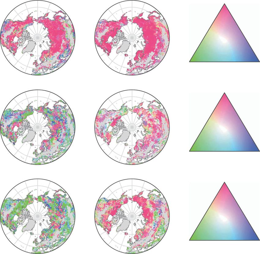
Fig. 5 Observed versus modeled vegetation growth carryover effects. Spatial patterns show the relative contributions of vegetation growth carryover
(VGC) and climatic factors of the present and preceding seasons to the interannual variations of Normalized Difference Vegetation Index (NDVI) or gross
primary productivity (GPP). Maps in the left column represent satellite-observed NDVI, and those in the right are the model ensemble-mean GPP for early
growing-season (EGS) (a, b), peak growing-season (PGS) (d, e), and late growing-season (LGS) (g, h). Ternary diagrams in c, f, i show the relative fraction
of global vegetated areas where the interannual trend of GPP (or NDVI) is dominated by each different driver (corresponding to the maps in each row).
Both percentages of the model ensemble-mean (closed blue circles) and the individual models (open symbols) and of satellite observation-based
estimates (closed black circles) are shown.
VGC (+)
VGC (+)
Warming (+)
Warming ( )
Enhanced growth
Strong warming and
Suppressed growth climate extremes ( )
Normal state
EGS PGS LGS Carryover to the next year
Accumulated soil water deficit
Fig. 6 Schematic representation of the vegetation growth carryover. The green curves indicate anomalies of vegetation greenness/productivity in
response to climatic changes and disturbances, relative to the climatological seasonal cycle (the gray line). Early growing-season (EGS) warming stimulates
extra vegetation growth and productivity, and this ecological benefit can persist into peak and late growing-season (PGS and LGS) and even the subsequent
year because vegetation growth is largely determined by its prior states (i.e., the vegetation growth carryover, VGC). This greening signal from EGS,
however, may be suppressed or even reversed for some locations due to climate extremes or soil moisture deficit legacy from EGS. The symbols − and +
in each bracket represent either a negative or positive force respectively imposed on terrestrial vegetation.
and LGS vegetation carbon sequestration, ultimately enhancing (Fig. 6). Processes involved in the lagged vegetation responses to
the annual carbon sink. However, it is important to bear in mind precedent climate, soil, and growth conditions are highly complex
that, while the beneficial VGC effect of EGS vegetation growth and often non-linear6,39,40. For example, summer climate
can override immediate and time-lagged climatic impact under extremes, which are often associated with large-scale climate
the present climate, whether this stronger VGC effect will con- oscillations and partly contributed by enhanced EGS vegetation
tinue with future warmer climate remains an open question growth25, could trigger severe tree mortality and fires that nullify
NATURE COMMUNICATIONS | (2021)12:983 | https://doi.org/10.1038/s41467-021-21223-2 | www.nature.com/naturecommunications 7ARTICLE NATURE COMMUNICATIONS | https://doi.org/10.1038/s41467-021-21223-2
any positive carryover effect from EGS (Fig. 6). Recent advances assimilated microwave observations of precipitation, surface-soil moisture, and
in statistical modelling and machine learning6,39,41 may provide vegetation optical depth (VOD)49. GLEAM incorporates VOD as this enables
estimates of the effects of water and heat stress and plant phenological changes on
useful tools for a better understanding of such non-linear vege- evapotranspiration49. This knowledge of vegetation response in turn allows char-
tation responses. acterisation of interactions between soil moisture and vegetation growth.
We also find poor representation of the VGC effect in dynamic
vegetation models, and as this likely influences predictive capacity EC measurements. We enhanced the reliability of remotely sensed seasonal
of future global carbon cycle changes, a major research challenge vegetation–climate interactions by additional analyses using monthly GPP esti-
is to better simulate biological processes related to this carryover mates and climatic variables from the FLUXNET2015 and AmeriFlux EC mea-
effect. Tackling this challenge requires not only using satellite and surements. EC-based GPP values used here were estimated from the direct
measurement of net ecosystem CO2 exchange by flux towers, combined with
ground measurements to refine existing parameterizations, but knowledge of plant light-response curves50. This FLUXNET2015 database consists
also using leaf-level measurements to understand the physiolo- of 212 sites that encompass 13 major vegetation types defined according to the
gical mechanisms controlling VGC patterns and to incorporate classification system of the International Geosphere Biosphere Programme (IGBP).
new process representation in model components. Long-term Here, we selected sites that provided at least 7 years of records, and excluded those
labeled as cropland or falling into MODIS-based regions dominated by cropland,
manipulative field experiments will also be useful to better leading to a total of 50 EC sites for analysis. Since launched in 1996, the AmeriFlux
characterize VGC features under different imposed meteorologi- observation network provides half-hourly or hourly flux records that allow for
cal regimes and to provide key process parameters for future temporal correlation analyses. We obtained a subset of 11 AmeriFlux sites (CA-
model improvements. TP4, US-Los, US-Me2, US-Ne1, US-Ne2, US-Ne3, US-PFa, US-Ton, US-Uaf, US-
Var, US-WCr) that provide at least 15 years of data, including GPP flux and
meteorological variables.
Methods
Satellite-based vegetation growth and land-cover maps. Normalized Difference
TRM chronologies. We obtained 2739 standardized TRM chronologies from the
Vegetation Index (NDVI) is commonly used as a proxy for vegetation greenness
International Tree-Ring Data Bank (ITRDB)51 V713 dating to August 2017. All
and photosynthetic activity. Here, NDVI data were obtained from the Global
selected tree-ring samples are located in the NH (>30°N), and cover at least 25
Inventory Monitoring and Modeling Studies (GIMMS) third-generation NDVI
years during 1901–2016. Each chronology is an average annual time series of
product (NDVI3g) based on retrievals from sensors on the Advanced Very High
standardized ring width measurements from typically 10 to 30 trees of the same
Resolution Radiometer (AVHRR)42,43. The GIMMS NDVI3g dataset is available at
species. We derived the standardized TRM series by detrending the raw TRM
a spatial resolution of 8 × 8 km2 and a biweekly temporal resolution, covering the
measurements based on the “cubic smoothing spline” approach52. This standar-
1982–2016 period. We composited the biweekly NDVI to monthly values by
dization removes low-frequency signals of wood growth associated with increasing
selecting the highest values.
tree age and trunk diameter, while still preserving interannual and interdecadal
Considering that NDVI may saturate in densely vegetated areas, we also
variabilities51. Site-level standard chronologies were generated by averaging tree-
included two other satellite-based products, LAI and GPP, to independently verify
level standardized tree ring indices with a bi-weight robust mean53.
the robustness of NDVI-based findings. Biweekly maps of the global land LAI were
derived from the GIMMS AVHRR LAI3g44, with a spatial resolution of 8 × 8 km2
for the period 1982–2016. The monthly gridded GPP maps at 0.5° spatial Process-based ecosystem model simulations. We used an ensemble of 16
resolution for 2001–2015 were derived from the remote sensing-based (RS) process-based terrestrial biosphere models participating in the TRENDY (trends in
product of the FLUXCOM database45,46. This dataset was generated with upscaling net land–atmosphere carbon exchange) v6 project29 that provide GPP outputs for
approaches based on three machine learning algorithms that integrated EC-based 1982–2016. These models were CABLE, CLM4.5, ISAM, JSBACH, JULES, LPJ-
carbon fluxes and satellite measurements from Moderate Resolution Imaging GUESS, LPJ-wsl, LPX-Bern, ORCHIDEE, ORCHIDEE-MICT, SDGVM, VISIT,
Spectroradiometer (MODIS)45,46. VEGAS, OCN, CLASS-CTEM, and DLEM (details in Supplementary Table 2). All
The effects of climate and VGC on vegetation changes can vary among these models performed the same set of factorial simulations following a standard
ecosystem types. Therefore, we investigated the climatic and VGC impacts experimental protocol29. In particular, we use TRENDY simulation S2 that was
separately for three major vegetation types of temperate grassland, forest forced by varying both atmospheric CO2 and climate. The historical climatic fields
(temperate and boreal), and arctic tundra and shrubland. We used the 300-m were from the CRU-NCEP V8 dataset, which is a merged product of monthly CRU
resolution global land-cover maps for 1992–2016 provided by the European Space observations and a 6-h NCEP reanalysis. Global atmospheric CO2 concentrations
Agency’s Climate Change Initiative (ESA-CCI)47 to delineate the three major were from a combination of ice-core records and the NOAA monitoring
vegetation types. These maps characterize the global surface using 37 land-cover observations.
classes defined by the United Nations Land Cover Classification System
(UNLCCS). We grouped the original UNLCCS classes into forest, shrub, and
grassland based on the cross-walking table provided by the ESA-CCI land cover Quantifying climatic and VGC effects on vegetation growth. We used satellite-
product47. We did not consider shrub as a separate group in temperate regions, but derived NDVI and concurrent climatic data to identify covariation between the
assigned this type evenly to grasses and forests. In this study, temperate grassland interannual variation of vegetation growth at northern latitudes (>30°N) of active
was defined as water-limited grassland distributed in warm mid-latitude regions, vegetation growing seasons (EGS, PGS, or LGS). We considered the NDVI of the
but excluding temperature-limited grassland in pan-Arctic regions and the Tibetan preceding season, as well as climatic variables (temperature and precipitation) of
Plateau. The forest type includes evergreen needleleaf forests, evergreen broadleaf both the focused season and the preceding season, as driving factors of seasonal
forests, deciduous needleleaf forests, deciduous broadleaf forests, and mixed forests. NDVI variations. Here we defined preceding-season NDVI for EGS as NDVI of the
The arctic tundra and shrubland was defined as temperature-limited grassland and preceding LGS rather than the preceding DS, since vegetation in DS is dormant and
shrubland over high latitudes (>50°N). We aggregated the land-cover maps into the detection of NDVI is hampered by the presence of snow cover (in cold regions).
0.5° resolution, and calculated the fraction of the above three vegetation types in Periods of different seasons were not defined for each grid cell directly by
each 0.5° grid. We only selected grid cells for which the dominant vegetation type temperature thresholds19 or fixed months across regions (e.g., spring as
occupied >60% of the grid area over the entire period of 1992–2016 March–May)25. Instead, we account for actual phenological seasonality using the
(Supplementary Fig. 9) to minimize potential confounding impacts of other climatological mean seasonal cycle of satellite-derived monthly NDVI values for
vegetation types and land cover conversions. We also masked northern ecosystems 1982–2016. We derived the dates for the start of the growing season (SOS) and the
dominated by cropland, as for these locations, the seasonal vegetation growth is end of the growing season (EOS) across the NH (>30°N) from the time when the
primarily controlled by human management practices such as irrigation, rate of the daily NDVI change interpolated from the original biweekly NDVI time
fertilization, cropping schedule, and multi-cropping, rather than environmental series was highest and lowest, respectively54. Our analysis is based on the 35-year
drivers. average of SOS and EOS, since we focus on interseasonal connections of mean
vegetation growth states (greenness or productivity) instead of the shift of
phenological events. PGS was defined as the two consecutive months with
Climatic and soil moisture data. Environmental variables used here include maximum NDVI values but not earlier than April or later than October. Grid cells
temperature, precipitation, and soil moisture. Monthly time series of temperature with maximum NDVI occurring before April or after October were not considered.
and precipitation were obtained from the Climatic Research Unit (CRU) v4.0.1 For regions with a growing season length of 3 months or less, PGS was defined as
dataset48. This gridded dataset, with a spatial resolution of 0.5°, was constructed by the month with the maximum NDVI value. Accordingly, EGS was defined as the
interpolation from meteorological stations based on spatial autocorrelation func- period from the month containing the SOS date to the beginning of PGS, and LGS
tions48. This climatic product also provides climatic forcing for TRENDY model was from the end of PGS to the month of EOS. The remaining months of a year
simulations, ensuring better comparability between observed and modeled were defined as the DS. Compared to seasonal descriptions based on temperature
responses of ecosystems to climate. Daily root-zone soil moisture estimates with a thresholds19 or fixed months25, these definitions of seasons utilizing the timing of
spatial resolution of 0.25° over 1988–2016 were derived from the Global Land phenological events are more suitable for analyzing linkages between different
Evaporation Amsterdam Model (GLEAM) v3.2a49. The GLEAM data have fully stages of vegetation growth in the active growing season. We aggregated monthly
8 NATURE COMMUNICATIONS | (2021)12:983 | https://doi.org/10.1038/s41467-021-21223-2 | www.nature.com/naturecommunicationsNATURE COMMUNICATIONS | https://doi.org/10.1038/s41467-021-21223-2 ARTICLE
NDVI for the three vegetation active seasons and then resampled the NDVI values may have on another, and is thus useful for exploring complex influence networks
to 0.5° to match the spatial resolution of the climatic data. The above definitions of in ecosystems. In this model, the causality between soil moisture and vegetation
seasons were also used for gridded EC measurements of GPP and climatic greenness is determined by the sign of their correlation. Positive correlations
variables. For site-level analyses, we derived SOS and EOS values based on the indicate a dominance of soil moisture impact on vegetation (soil moisture
derivative of the time series of daily GPP (i.e., the maximal/minimum second stimulates growth), while negative correlations indicate a dominance of vegetation
derivative value as the SOS/EOS55) that were smoothed with spline curves. impact on soil moistures (growth depletes soil moisture). We used the χ2 test (and
We quantified the contributions of climatic drivers (present- and preceding- associated p values), the root mean square error of approximation (RMSEA), and
season for both temperature, TMP and precipitation, PRE) and VGC (preceding- an adjusted goodness-of-fit index (AGFI) to evaluate the fit of the established SEM
season NDVI) to observed NDVI trend during 1982–2016. This quantification was models. The SEM analysis was implemented using the AMOS (version 21.0)
achieved by decomposing the 35-year linear trend of NDVI (dNDVI dt ) for each season
software (Amos Development Corporation, Chicago, USA).
into the additive contributions of five components:
dY ∂Y dYps ∂Y dTMPps ∂Y dPREps ∂Y dTMP ∂Y dPRE Data availability
¼ þ þ þ þ þε All observation and model data that support the findings of this study are available as
dt ∂Yps dt ∂TMPps dt ∂PREps dt ∂TMP dt ∂PRE dt
follows. The AVHRR GIMMS NDVI3g data are available at http://ecocast.arc.nasa.gov/
¼ ΔY Yps þ ΔY TMPps þ ΔY PREps þ ΔY TMP þ ΔY PRE þ ε ¼ ΔY Yps þΔY CLMps þ ΔY CLM þ ε
data/pub/gimms/3g.v0/; The AVHRR GIMMS LAI3g data are available at http://cliveg.
ð1Þ bu.edu/modismisr/lai3g-fpar3g.html; The FLUXCOM RS GPP product is available at
∂Y http://www.fluxcom.org/; The ESA-CCI land-cover maps are available at http://maps.elie.
where represents the sensitivity of Y (NDVI) to an explanatory variable X
∂X ucl.ac.be/CCI/viewer/download.php; The climatic variables from the CRU v4.0.1 data are
(NDVIps, TMPps, PREps, TMP, or PRE). These sensitivities were estimated as the available at https://crudata.uea.ac.uk/cru/data/hrg/; The FLUXNET2015 EC
regression coefficients of a multiple linear regression performed with NDVI against measurements are available at https://fluxnet.fluxdata.org/2015/12/31/fluxnet2015-
all listed explanatory variables for 1982–2016. dY dX
dt (or dt ) represents the linear trend dataset-release/; The AmeriFlux EC measurements are available at https://ameriflux.lbl.
of Y (or X) during 1982–2016. For different seasons, this trend was calculated as gov/data/download-data/; The tree-ring width chronologies from the ITRDB V713 data
the slope of the simple linear regression of mean Y (or X) values against the year. are available at https://www.ncdc.noaa.gov/data-access/paleoclimatology-data/datasets/
Here, The NDVI trend during 1982–2016 (dY dt ) was decomposed into the tree-ring/; the root-zone soil moisture from the GLEAM v3.2a data are available at
contribution of each variable X (ΔYX), which was represented as the product of the https://www.gleam.eu/; model outputs generated by TRENDY v6 ecosystem models are
partial derivative against that variable X as ∂Y
∂X and the concurrent trend of X itself as available from Stephen Stich (s.a.sitch@exeter.ac.uk) or Pierre Friedlingstein (p.
dX
dt . Note that the contributions of temperature and precipitation were combined to
friedlingstein@exeter.ac.uk) upon request.
provide the total contribution of climate change to the trend of NDVI, for both the
preceding season (ΔY CLMps ) and the present season (ΔY CLM ). ε represents the
Code availability
difference between the observed and predicted Y. The approach given by Eq. (1)
The processing MATLAB codes are available from the corresponding author upon
was conducted for each grid cell, and the total areally-averaged contribution of
request.
each factor to the trend of NDVI over the NH was calculated by averaging the
decomposed contribution of factors (ΔYX) across all the northern vegetated
nonagricultural areas. In addition to satellite-observed analyses, we also conducted Received: 29 August 2020; Accepted: 19 January 2021;
similar analyses with TRENDY model simulated GPP. The analyses were similar to
that of NDVI-based, except that GPP was used to represent vegetation growth as
the dependent variable.
We also applied a partial correlation analysis to assess the relationship between
seasonal time series of NDVI and each driving factor while statistically controlling
for potential covarying effects of the remaining set of factors. This analysis was References
performed for NDVI values averaged over the entire NH (30–90°N) (Fig. 1) and 1. Thayer, Z. M. & Kuzawa, C. W. Biological memories of past environments:
that for each pixel (Supplementary Figs. 1 and 4–6). epigenetic pathways to health disparities. Epigenetics 6, 798–803 (2011).
At the annual time scale, we again calculated partial correlations between 2. Ogle, K. et al. Quantifying ecological memory in plant and ecosystem
NDVI of each year and that of the preceding year (and similarly for TRW), while processes. Ecol. Lett. 18, 221–235 (2015).
statistically factoring out the covarying effects of climatic factors (temperature 3. Harrison, X. A., Blount, J. D., Inger, R., Norris, D. R. & Bearhop, S. Carry-over
and precipitation of the present and preceding year). For comparability with effects as drivers of fitness differences in animals. J. Anim. Ecol. 80, 4–18
standardized tree ring data, linear trends of all yearly time series were removed. (2011).
Additionally, we quantified the persistence of the interannual VGC by 4. O’Connor, C. M., Norris, D. R., Crossin, G. T. & Cooke, S. J. Biological
calculating partial autocorrelation coefficients20 of NDVI and TRW time series, carryover effects: linking common concepts and mechanisms in ecology and
but with the lead time ranging from 1 to 3 years. For example, for a lead time j evolution. Ecosphere 5, art28 (2014).
(years), we calculated the partial correlation between Yt (NDVI or TRW, t is the 5. Hughes, T. P. et al. Ecological memory modifies the cumulative impact of
present time) and Yt−j, while factoring out the covarying effects of all smaller recurrent climate extremes. Nat. Clim. Change 9, 40–43 (2018).
lead periods (0, 1, 2, …, j−1). 6. Besnard, S. et al. Memory effects of climate and vegetation affecting net
As a further check of the detected NDVI-based seasonal ecosystem responses to ecosystem CO2 fluxes in global forests. PLoS ONE 14, e0211510 (2019).
different drivers, we also plotted the trend of GPP against that of climatic factors 7. Peterson, G. D. Contagious disturbance, ecological memory, and the
preceding-season GPP across all FLUXNET EC sites (Fig. 3). The majority of these emergence of landscape pattern. Ecosystems 5, 329–338 (2002).
EC sites are distributed in temperate climates with relatively homogeneous trends 8. Piao, S. L. et al. Interannual variation of terrestrial carbon cycle: issues and
of temperature. Thus these sites alone do not encompass sufficient spatial perspectives. Glob. Change Biol. 26, 300–318 (2020).
variations of GPP response to warming. However, the sensitivity of GPP to 9. Comas, L. H., Becker, S. R., Cruz, V. M. V., Byrne, P. F. & Dierig, D. A. Root
temperature varies across sites of different ecosystem types. We therefore plotted traits contributing to plant productivity under drought. Front. Plant Sci. 4, 442
the trend of GPP against the calculated temporal sensitivity of GPP to temperature (2013).
across these EC sites, to understand such ecosystem dependence. For the 11 10. Bernhardt-Römermann, M. et al. Functional traits and local environment
Ameriflux EC sites with sufficient temporal coverage, we quantified the partial predict vegetation responses to disturbance: a pan-European multi-site
correlations between time series of GPP and that of its driving factors, in the same
experiment. J. Ecol. 99, 777–787 (2011).
manner as that conducted for satellite-observed NDVI.
11. Jump, A. S. et al. Structural overshoot of tree growth with climate variability
In Eq. (1), residual ε represents the contributions of other drivers that could
and the global spectrum of drought-induced forest dieback. Glob. Change Biol.
influence vegetation growth but were not included in this regression. The above
23, 3742–3757 (2017).
analyses focus on the influence of factors in the concurrent and the immediately
previous season on seasonal vegetation growth. An additional analysis was also 12. Murray-Tortarolo, G. et al. Evaluation of land surface models in reproducing
performed to extend the time period to the entire previous year except the satellite-derived LAI over the high-latitude Northern Hemisphere. Part I:
immediately neighboring season, by correlating the residual series with the same uncoupled DGVMs. Remote Sens. 5, 4819–4838 (2013).
factors of the previous seasons. For example, for ε of PGS NDVI, we calculated its 13. Smith, W. K. et al. Large divergence of satellite and Earth system model
correlation with NDVI, TMP, and PRE of the previous PGS and LGS, and TMP estimates of global terrestrial CO2 fertilization. Nat. Clim. Change 6, 306–310
and PRE of the previous DS (Supplementary Fig. 7). (2016).
We also used SEM to assess the direct and indirect pathways of how climatic 14. Liu, Y., Schwalm, C. R., Samuels-Crow, K. E. & Ogle, K. Ecological memory of
factors and VGC influence vegetation changes across seasons for the three major daily carbon exchange across the globe and its importance in drylands. Ecol.
vegetation types. SEM is a multivariate statistical approach that synthesizes path, Lett. 22, 1806–1816 (2019).
factor, and maximum-likelihood analyses, and provides strong pointers to 15. Oesterheld, M., Loreti, J., Semmartin, M. & Sala, O. E. Inter-annual variation
underlying deterministic processes. Compared with traditional multivariate in primary production of a semi-arid grassland related to previous-year
analyses, SEM allows partitioning the direct and indirect effects that one variable production. J. Veg. Sci. 12, 137–142 (2001).
NATURE COMMUNICATIONS | (2021)12:983 | https://doi.org/10.1038/s41467-021-21223-2 | www.nature.com/naturecommunications 9You can also read