What Does "Below, but Close to, 2 Percent" Mean? Assessing the ECB's Reaction Function with Real-Time Data
←
→
Page content transcription
If your browser does not render page correctly, please read the page content below
What Does “Below, but Close to, 2 Percent”
Mean? Assessing the ECB’s Reaction Function
          with Real-Time Data∗

       Maritta Paloviita, Markus Haavio, Pirkka Jalasjoki,
                       and Juha Kilponen
                               Bank of Finland

           Using unique real-time quarterly macroeconomic projec-
       tions of the Eurosystem/ECB staff, we estimate competing
       specifications of the ECB’s monetary policy reaction function.
       We consider specifications which include inflation and output
       growth projections, a past inflation gap, a time-varying nat-
       ural real interest rate, and different inflation targets. Our first
       key finding is that the de facto inflation target of the ECB lies
       between 1.6 percent and 1.8 percent. Our second key finding is
       that the ECB reacts both to short-term macroeconomic pro-
       jections and to past deviations of inflation from its de facto
       target.
       JEL Codes: E31, E52, E58.

   ∗
    All authors are from the Bank of Finland. We are indebted to Giacomo Car-
boni, Seppo Honkapohja, Aki Kangasharju, Jarmo Kontulainen, Tomi Kortela,
Mika Kortelainen, Athanasios Orphanides, Antonio Rua, and Tuomas Välimäki
for valuable comments and suggestions. We are also grateful for constructive
suggestions received at a seminar organized by the National Bank of Belgium,
the XL Annual Meeting of the Finnish Economic Association, ECB Working
Group of Forecasting meeting, Bank of Russia Conference on Inflation: New
Insights for Central Banks, 15th Euroframe Conference on Economic Policy
Issues in the European Union, Cracow University of Economics Workshop on
Macroeconomic Research, MMF 50th Annual Conference, ECB Monetary Policy
Committee Meeting, National Bank of Poland Research Seminar, Bank of Fin-
land Monetary Policy Seminar, and Nordic Monetary Policy Meeting. The views
expressed in this paper are those of the authors and do not necessarily reflect the
views of the Bank of Finland or the Eurosystem. Corresponding author e-mail:
maritta.paloviita@bof.fi.

                                       125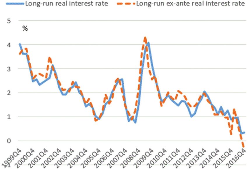
126            International Journal of Central Banking               June 2021

1.       Introduction

In recent years, inflation has been persistently low in many
economies. As a response, policy rates have been cut to very low lev-
els, and new measures have been introduced to maintain an accom-
modative stance of monetary policy. The low inflation and interest
rate environment have raised the question of whether and how the
current monetary policy framework should be reformed (see, e.g.,
Bernanke 2017a, 2017b; Williams 2017; Bullard 2018; Honkapohja
and Mitra 2018). In the case of the European Central Bank, there
has also been a vivid debate on the precise numerical target for
inflation and possible asymmetry of the ECB’s policy responses.
    The debate on the ECB’s price stability objective stems from the
fact that its inflation aim is not precisely defined in the Treaty on
the Functioning of the European Union. In 1998, the ECB’s Gov-
erning Council defined price stability as a “year-on-year increase in
the Harmonised Index of Consumer Prices (HICP) for the euro area
of below 2%.” In 2003, the Governing Council clarified that “in the
pursuit of price stability it aims to maintain inflation rates below,
but close to, 2% over the medium term.” This clarification can be
seen as an effort to reduce uncertainty about the lower bound of the
inflation aim relative to the earlier definition and to provide a buffer
against large negative shocks to inflation.
    As discussed in Hartmann and Smets (2018), the exact formu-
lation by the Governing Council in 2003 was a compromise that
maximized that buffer while remaining consistent with the defin-
ition of price stability. With this reformulation, the inflation aim
remained nevertheless ambiguous.1 In particular, although the ECB
communication stresses symmetry, the expression “below, but close
to 2%” has some feel of asymmetry, and the exact numerical target
is not spelled out.2

     1
     Apel and Claussen (2017) classify three different categories for inflation tar-
geting. A point target refers to a single number. If certain deviations from the
point target are “acceptable” for the central bank, it is complemented with a
tolerance band. In the case of a target range, a targeted inflation interval is
announced without any specific desirable level of inflation.
   2
     According to the ECB strategy, “the Governing Council’s aim to keep euro
area inflation below, but close to, 2% over the medium term signifies a com-
mitment to avoiding both inflation that is persistently too high and inflation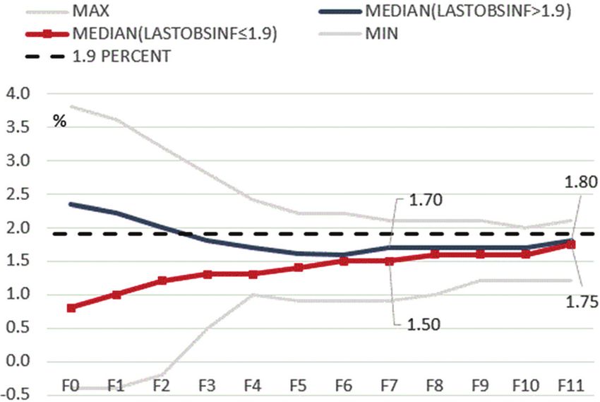
Vol. 17 No. 2   What Does “Below, but Close to, 2 Percent” Mean?          127

    Not surprisingly, the ECB’s inflation aim has been interpreted
in various ways. For example, Miles et al. (2017) point out that the
ECB’s “target itself is perceived as asymmetric.” They also note
that there “is uncertainty about what ‘close to, but below’ means.”
Regarding the public, survey evidence indicates that households’
knowledge about the ECB’s inflation target is “far from perfect”
(van der Cruijsen, Jansen, and de Haan 2015). Different interpreta-
tions of the inflation target and/or vague monetary policy communi-
cation may increase inefficiency in monetary policymaking, give rise
to risks of deanchored inflation expectations, and, hence, jeopardize
the effective transmission of monetary policy. After introducing new
policy measures, the ECB has strengthened its communication and
adopted a forward-guidance framework in order to reduce uncer-
tainty concerning its reaction function and future policy actions.3
    In this paper, we are specifically interested in assessing the ECB’s
own interpretation of the price stability objective and its reaction
function. Using unique real-time quarterly macroeconomic projec-
tions of the Eurosystem/ECB staff, we attempt to quantify the gist
of the expression “below, but close to 2%.” First, we consider the
levels toward which the ECB inflation projections converge in the
medium term. Second, we estimate a large number of alternative
output-growth-gap-based reaction functions in order to directly infer
the ECB’s de facto inflation target. Finally, using primarily the real
gross domestic product (GDP) growth as a cyclical variable, we esti-
mate more general reaction function specifications, which allow the
ECB to react (either symmetrically or asymmetrically) also to past
inflation gaps, determined by the deviations of realized inflation from
the de facto target. In all cases, we pay special attention to the
relevant forecast horizon in monetary policymaking.
    A novel feature of our analysis is that our data set includes
the Eurosystem/ECB staff quarterly macroeconomic projections of
inflation and real GDP growth made in 1999–2016. Consequently,

that is persistently too low.” For example, in March 2016 Mario Draghi, Pres-
ident of the European Central Bank, stated: “The key point is that the Gov-
erning Council is symmetric in the definition of the objective of price stabil-
ity over the medium term.” (https://www.ecb.europa.eu/press/pressconf/2016/
html/is160310.en.html.) See also President Draghi’s speech of June 2016, at
https://www.ecb.europa.eu/press/key/data/2016/html/sp160602.en.html.
   3
     See, e.g., Cœuré (2017).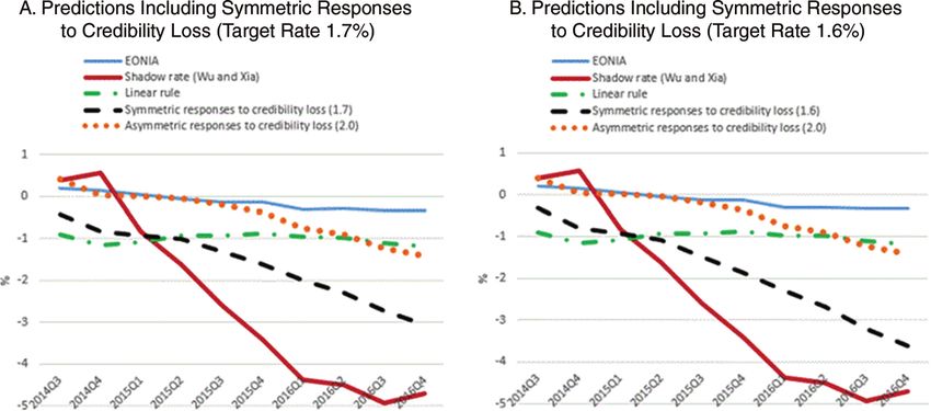
128          International Journal of Central Banking            June 2021

we are able to estimate the reaction function with a subset of the
very same information the Governing Council has available when it
decides on the monetary policy stance.4 As emphasized by Wood-
ford (2007), an important feature of “optimal” monetary policy is
that it should respond to the projected future path of the economy
and not only to current conditions.
    Our sample period, 1999:Q4–2016:Q4, covers the relatively stable
pre-crisis years as well as the recent turbulent years characterized by
the financial crisis, the sovereign debt crisis, and low inflation. Using
subsample analysis and recursive estimations, we analyze the stabil-
ity of estimated parameters of the ECB’s reaction function over time.
In addition to the targeted rate of inflation, we conduct a robust-
ness analysis with respect to the time span of forward-looking and
backward-looking variables in the reaction function and with respect
to time-varying long-run natural real interest rates. We assess the
performance of estimated reaction functions by comparing their in-
sample predictions against the key interest rates. In the analysis
of the most recent period when standard interest rate policy has
approached its effective lower bound, we evaluate the performance
of our estimated functions by comparing their out-of-sample predic-
tions against shadow interest rates estimated by Kortela (2016) and
by Wu and Xia (2016).
    Our extensive analyses based on alternative approaches and
unique real-time data indicate that the de facto inflation target of
the Governing Council lies between 1.6 percent and 1.8 percent. This
finding is consistent with the fact that the Eurosystem/ECB staff
medium-term inflation projections have had a tendency to converge
rapidly on values well below 2 percent. We also find that the ECB
conditions its interest rate decisions not only on short-term macro-
economic projections but also on past inflation developments. This
is also consistent with the recent ECB communication, according to
which the launch of asset purchase programs can be justified as a
response to too-prolonged a period of low inflation. Finally, we find

   4
     To our knowledge, earlier reaction function estimations using the ECB’s
projections have been based on annual information only, with one exception:
Hartmann and Smets (2018). Fischer et al. (2009) examine euro-area monetary
analysis in 1999–2006 using quarterly information.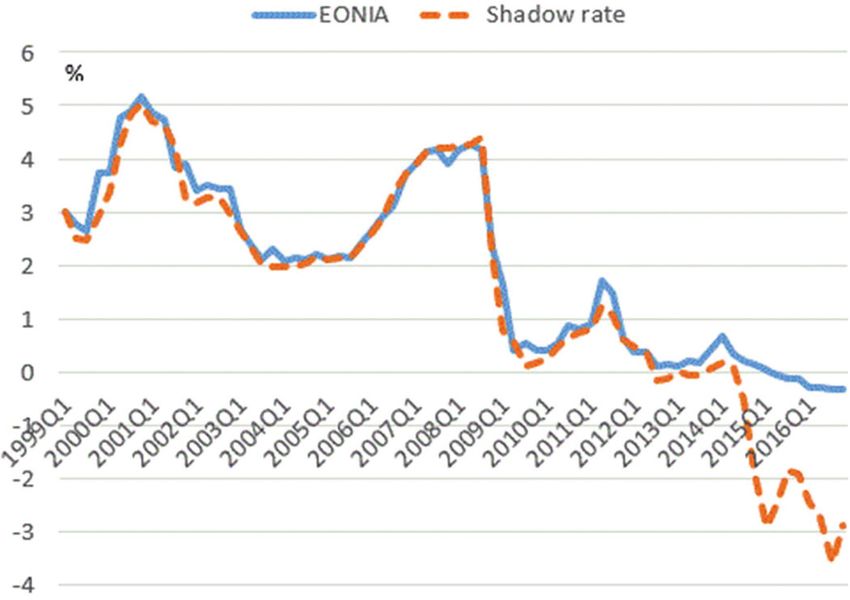
Vol. 17 No. 2   What Does “Below, but Close to, 2 Percent” Mean?      129

some evidence of asymmetry in policy rules in which we fix the infla-
tion target to 2 percent. However, the out-of-sample predictions of
the symmetric reaction function with a low de facto target outper-
form the asymmetric reaction function during the zero lower bound
period.
    In earlier studies, euro-area monetary policy has also been widely
examined using alternative specifications of the classical Taylor rule
(Taylor 1993).5 Monetary policy analysis has often been based on
real-time information. As a proxy for real-time information, the ECB
Survey of Professional Forecasters (ECB SPF) (e.g., Gerlach and
Lewis 2014) and Consensus Forecast (e.g., Gorter, Jacobs, and de
Haan 2008) have been used. Some authors have also used the ECB’s
macroeconomic projections (e.g., Belke and Klose 2011; Bletzinger
and Wieland 2017). As the ECB projections were published only
for full calendar years until 2017, quarterly variation in the pro-
jections has been taken into account in reaction function estima-
tions so far only by Hartmann and Smets (2018). Close to our study
also is an article by Bletzinger and Wieland (2017), who also esti-
mate a forecast-based reaction function for the euro area in order
to assess the targeted level of inflation and the ECB policy dur-
ing the zero lower bound period. Their analysis is based on the
ECB SPF survey and the ECB projections for full calendar years.
The main difference from our approach is that they do not take
into account the impact of past inflation deviations from the target,
and their cyclical variable is defined as a difference between output
growth and the European Commission’s estimate of potential output
growth.6
    The paper is organized as follows. The Eurosystem/ECB staff
projections are described and their medium-term convergence is
examined in section 2. Alternative specifications of the monetary
policy reaction function and estimation results are presented in
section 3. In section 4, we discuss in-sample and out-of-sample pre-
dictions of different reaction functions. Concluding remarks are pro-
vided in section 5.

  5
    See, e.g., Clarida, Galı́, and Gertler (1998).
  6
    Earlier studies of possible asymmetries in ECB monetary policy include
Surico (2003, 2007), Aguiar and Martins (2008), and Ikeda (2010).
130           International Journal of Central Banking                June 2021

2.       The Data and Eurosystem/ECB Staff Projections

2.1      Data Description
Our data set includes the real-time Eurosystem/ECB staff projec-
tions made in 1999:Q4–2016:Q4 for the euro-area year-on-year HICP
inflation rate and year-on-year real GDP growth rate. These projec-
tions are publicly available as annual data for full calendar years,
but our analyses are based on confidential quarterly information.7
    For both the inflation rate and real GDP growth rate our
data include real-time estimates of previous-quarter values, current-
quarter values (nowcast estimates), and real-time projections until
the end of each forecast horizon. The projections in our data cover
the current and next two calendar years. The “final” data, i.e.,
revised data, for our purposes, are the latest available vintages pub-
lished by Eurostat in the spring of 2017. The euro-area GDP data
are seasonally and working-day adjusted.
    Projection errors increase substantially with the length of the
forecast horizon, reflecting real-time challenges in actual monetary
policymaking.8 The mean errors (ME) for the one- to four-quarters-
ahead inflation projections (real GDP growth projections) are −0.02,
−0.06, −0.11, and −0.13 (−0.11, 0.07, 0.29, and 0.51). The corre-
sponding root mean squared errors (RMSE) for inflation are 0.37,
0.59, 0.78, and 0.95 and for real GDP growth 0.96, 1.33, 1.68,
and 1.96. A limited forecast accuracy in the medium to long term
is not specific to the ECB and the Eurosystem. Charemza and
Ladley (2016) have analyzed inflation forecasts made in 2000–11
in 10 inflation-targeting central banks (the ECB is not included
in the study). They show that compared with the CESifo World
Economic Survey forecasts, the central banks’ one-year-ahead infla-
tion forecasts are biased toward the inflation target. According to
their analysis, the bias is even stronger in two-years-ahead inflation
forecasts.9

     7
     See Alessi et al. (2014) and ECB (2016) for a detailed description of the
Eurosystem/ECB staff projections exercises.
   8
     We define projection errors as the difference between projections and real-
izations.
   9
     Charemza and Ladley’s (2016) analysis includes 10 inflation-targeting central
banks: Australia, Canada, Chile, Czech Republic, Korea, Mexico, New Zealand,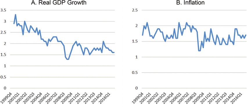
Vol. 17 No. 2    What Does “Below, but Close to, 2 Percent” Mean?            131

    Our data set also includes the EONIA (euro overnight index
average) interest rate, the MRO (main refinancing operations) rate,
and shadow interest rates estimated by Kortela (2016) and Wu and
Xia (2016).10 The shadow rates follow closely the EONIA rate until
about mid-2014, but thereafter they start to fall strongly into a neg-
ative territory, reflecting the quantitative easing of the ECB (see
figure A.1 in appendix A).
    We also calculate several time-varying ex ante and ex post prox-
ies of the long-run natural real interest rate, which are constructed
using yields on German government bonds of different maturities or
a composite nominal yield of 10-year euro-area government bonds.
The composite nominal yield is constructed by the ECB by aggre-
gation using GDP weights. We use these different proxies of the
natural rate because of measurement issues. Differences in long-
term bond yields of different euro-area economies were small until
around the inception of global financial crisis in our sample, so it
does not make a great difference whether the German government
bonds or composite yield is used for that period. Since about 2007,
however, the difference becomes significant, and the German gov-
ernment bond yields are likely to be a better proxy for the euro-
area risk-free nominal rate, as it corresponds to the lowest of the
10-year government bond yields. However, this is not necessarily
the best proxy for the euro-area long-run natural rate, i.e., for
the rate which would stabilize the euro-area economy as a whole,
in the long run. The literature in general uses either short-term
bond yields or long-term bond yields to approximate the natural
rate.

Norway, Poland, and Sweden. See Sveriges Riksbank (2017) for the accuracy of
Riksbank’s inflation forecasts.
  10
     A shadow rate is a summary measure of monetary policy stance, capturing
unconventional as well as conventional policy measures. It indicates how much
the central bank would have lowered the interest rates had the zero lower bound
not been binding, i.e., it reflects monetary policy stance in very low or negative
interest rate environments. Differences between alternative shadow rates for the
euro area based on different methods are typically quite large. However, they all
indicate that the ECB’s monetary policy stance has recently been very accom-
modative. In Kortela (2016), the shadow rate is based on a multifactor shadow
rate term structure model (SRTSM) with a time-varying lower bound.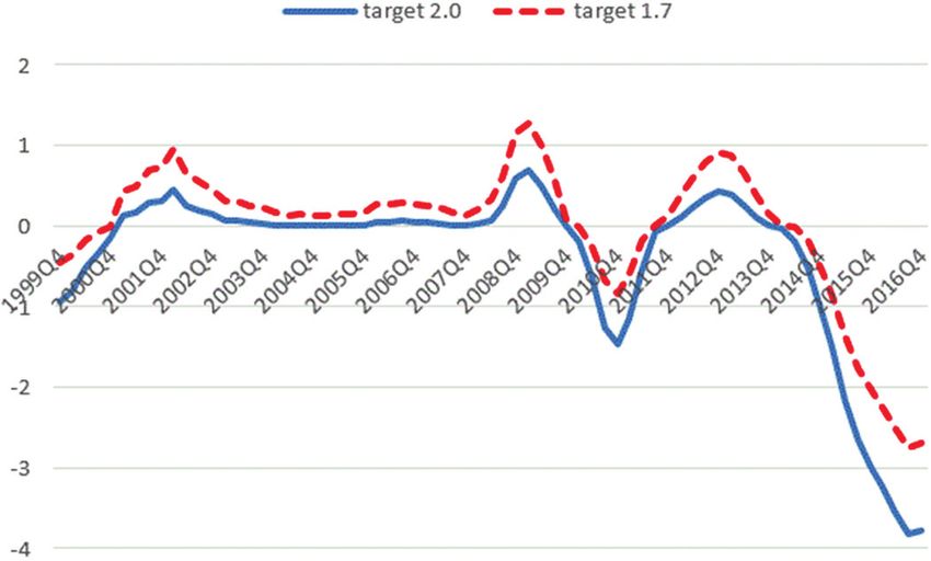
132             International Journal of Central Banking              June 2021

2.2     Medium-Term Convergence of Inflation and Output
        Growth Projections
The Eurosystem/ECB staff inflation projections provide suggestive
evidence of the ECB’s de facto inflation target. Projected values of
the economic variables, including inflation, at the end of the forecast
horizon are largely determined by the models’ long-run equilibriums,
i.e., values to which they are expected to converge in the absence
of new shocks hitting the economy. This is important for the deter-
mination of inflation itself, since empirical literature largely agrees
that the central bank forecasts have an impact on the private sector’s
inflation forecasts and expectations.11 It is important to note that
the ECB inflation projections are conditioned on market expecta-
tions of the interest rate (since June 2006) and not on some “optimal
state contingent path of the interest rates.” Therefore, the projected
inflation does not reflect the ECB’s desired path of inflation per se.
However, one can plausibly argue that the projected inflation rates
at the end of the forecast horizon give the public a good guideline for
inflation which the ECB considers consistent with its mandate. This
is supported by the fact that inflation forecasts have typically con-
verged to the promixity of “close but below two” already after about
six quarters. There is rather little movement in inflation forecasts
thereafter, as we show below.
     Figure 1 illustrates the inflation projections. It shows two sep-
arate medians of the inflation projections based on whether the
latest observed inflation rate during each projection exercise has
been above or below 1.9 percent. More precisely, we have organized
the projection data in figure 1 in the following way: the label “F0”
on the horizontal axis refers to the median value of nowcast esti-
mates from all the projection vintages and the labels “F1”–“F11”
refer to the median values of the corresponding inflation projections
for 1–11 quarters ahead. In addition to the medians, figure 1 also
presents the highest and lowest inflation projections for different
forecast horizons.
     Figure 1 shows that the medians of projections made at times
when the recent observed inflation rate is high (i.e., higher than

 11
      See, e.g., Fujiwara (2005), Hubert (2015), and Lyziak and Paloviita (2018).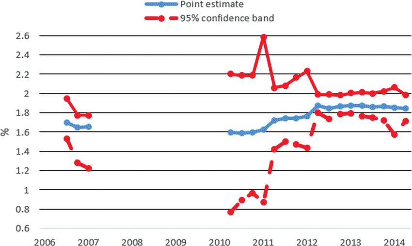
Vol. 17 No. 2   What Does “Below, but Close to, 2 Percent” Mean?          133

  Figure 1. Median Inflation Projections Conditioned on
          Latest Observed Inflation Rate during
                 Each Projection Exercise

Sources: ECB and authors’ own calculations.
Notes: On the horizontal axis, the label “F0” refers to the real-time current-
quarter nowcasts and the label “F1” to the one-quarter-ahead projections, etc.
The curves “MAX” and “MIN” refer to the highest and lowest inflation projec-
tions made in 1999:Q4–2016:Q4.

1.9 percent) converge to 1.70–1.80 percent after six quarters. At the
same time, however, the medians of projections starting from lower
inflation conditions (i.e., 1.9 percent or lower) converge to slightly
lower rates around 1.60–1.75 percent. Lower medians converge to
their eventual rates in a rather linear fashion, while the evolution
of the higher medians has a somewhat different shape: the median
projections for five and six quarters ahead are slightly below the
medians at the end of the forecast horizon, i.e., inflation is projected
to temporarily undershoot when inflation has been initially above
1.9 percent.
    It is notable in figure 1 that regardless of the current level of
inflation, after about six quarters the median inflation projections
are already in the proximity of their levels at the end of the fore-
cast horizon. When compared with the actual realized inflation, the
134 International Journal of Central Banking June 2021
Figure 2. Medium-Term Projections
Sources: ECB and authors’ own calculations.
Note: The graphs present the real GDP growth and inflation projections for the
last quarter of the projection horizon for each projection exercise (the horizontal
axis).
projected inflation exhibits stronger and faster mean reversion. Sim-
ilarly to the inflation forecasts, the GDP growth forecasts also have
a tendency to revert very quickly back to the perceived long-run
growth rate. As a result, in both cases of inflation and GDP growth,
the sample standard errors are much higher than the standard errors
computed from different forecast vintages, especially at the end of
the forecast horizon (see table A.1 in appendix A).
The medium-term real GDP growth and inflation projections are
summarized in figure 2. The GDP growth projections do not revert
toward a single long-run value over the sample, but rather the pro-
jections seem to capture the slowdown of long-run growth rates over
the sample period. While at the beginning of the sample the GDP
growth projections converged to growth rates of around 2.5 percent,
more recently the projections have converged to below 2 percent
growth. This decline in the projected medium-term growth rate is
consistent with the trendlike decline in the real interest rates (see
figure A.2 in appendix A), and also with the more recent Eurosys-
tem’s view that the potential growth of the euro-area economy is
in the proximity of 1.5 percent. In contrast to the medium-term
GDP growth forecasts, the inflation forecasts do not show a similar
downward trend.Vol. 17 No. 2 What Does “Below, but Close to, 2 Percent” Mean? 135
3. Estimation of the ECB Reaction Function
In what follows, we estimate alternative specifications of the
Eurosystem/ECB’s reaction functions for the period 1999:Q4–
2014:Q2 (i.e., until the zero lower bound was reached) and assess
the ECB’s de facto inflation target both directly and indirectly. In
our extensive analysis, we pay special attention to real-time data
challenges and we also focus on possible backward-looking features
of the monetary policy decisions.
We proceed in two steps. We first consider simple output-growth-
gap-based (Taylor-type) reaction functions, which allow us to cal-
culate the ECB’s implied inflation target based on the estimated
parameters. Then, in section 3.2, we consider less standard specifi-
cations where we use output growth as a cyclical variable due to the
difficulty of estimating the output gap in real time and the fact that
the ECB’s communication is based more on the current and future
output growth than on the output gap (see, e.g., Orphanides and
van Norden 2002, Gerlach 2007, Orphanides 2008).12 Using these
specifications, we are able to assess the value of the ECB’s de facto
inflation target indirectly.13
When estimating nonstandard specifications of the reaction func-
tion in section 3.2, we consider possible backward-looking features in
the ECB monetary policymaking by following Neuenkirch and Till-
mann (2014)14 : we augment our forward-looking specifications with
a backward-looking inflation gap term, which measures how strongly
actual inflation has deviated on average from the presumed inflation
target in recent quarters. This past inflation gap—i.e., a “credibility
loss term”—is specified as
CLt = (π̄t−1,t−q − π ∗ )|π̄t−1,t−q − π ∗ |. (1)
12
For the euro area, the problem of reliable real-time output gap estimates is
especially severe, due to a relatively short sample and methodological issues that
arise from calculating the real-time output gap based on country aggregations
(Marcellino and Musso 2011).
13
Output-growth-based reaction functions have been analyzed by several
authors. See, for example, Gorter, Jacobs, and de Haan (2008), Sturm and de
Haan (2011), Gerlach and Lewis (2014), and Neuenkirch and Tillmann (2014).
14
Neuenkirch and Tillmann (2014) analyze monetary policy in five inflation-
targeting economies: Australia, Canada, New Zealand, Sweden, and the United
Kingdom.136 International Journal of Central Banking June 2021
π̄t−1,t−q refers to an average past inflation rate and q to the
number of lags. The CL term is specified such that it penalizes both
negative and positive deviations of average past inflation from the
target symmetrically. For instance, if average past inflation is 1 per-
centage point below or above the target, in both cases the CL term
gets the same absolute value but the sign is different. The absolute
value term in equation (1) weights large deviations of inflation from
the target more than small ones, hence the term is nonlinear. This
nonlinear feature is needed to make indirect inference on the de facto
inflation target.
This CL term, if found significant, introduces history dependence
in the ECB policymaking. Past inflation developments may play a
role in monetary policy setting because of various reasons. First, if
the actual inflation rate has been below (above) the inflation target
over a long period of time, the central bank may need to aim for a
slightly faster (slower) rise in prices in the near future in order to
achieve the inflation target in the medium term. This implies more
accommodative (tighter) policy than what the current economic out-
look would otherwise imply (see, e.g., Woodford 2007). Second, if
inflation has persistently deviated from the target, the central bank
may react more aggressively than would be required by information
based on purely macroeconomic forecasts to maintain its credibility
and commitment to the target. In this case, monetary policy aims
to ensure that general (longer-term) inflation expectations remain
anchored to the central bank’s inflation target (see, e.g., Ehrmann
2015, Lyziak and Paloviita 2017). The third possible interpretation
relates to unconventional monetary policy and, above all, to forward
guidance: in the context of persistently low inflation, the central
bank may promise to keep monetary policy accommodative even
after monetary policy should be tightened according to the current
economic outlook. This kind of forward guidance may appear in the
reaction function as a link between the current policy rate and past
inflation.15
15
Cœuré (2017) argues that the ECB’s forward guidance is based on a struc-
tural component that corresponds to the ECB reaction function and a variable
component which consists of evolving economic outlook. According to him, the
reaction function “includes the mapping of any desired monetary policy stance
into instruments, such as policy rates and asset purchases.”Vol. 17 No. 2 What Does “Below, but Close to, 2 Percent” Mean? 137
Figure A.3 in appendix A presents the evolution of the ECB’s
CL term for the inflation targets of 1.7 percent and 2.0 percent,
using seven lags over which the average past inflation π̄t−1,t−7 is
measured. Both measures indicate that in the mid-2000s, past infla-
tion gaps were minor, while more pronounced past inflation gaps are
measured around 2002, 2009, 2011, and 2013, and again after 2014
when the nominal interest rate hit the lower bound and inflation
slowed down persistently. The relatively large inflation gaps espe-
cially in the post-crisis period may have had a significant impact on
the ECB’s monetary policy.
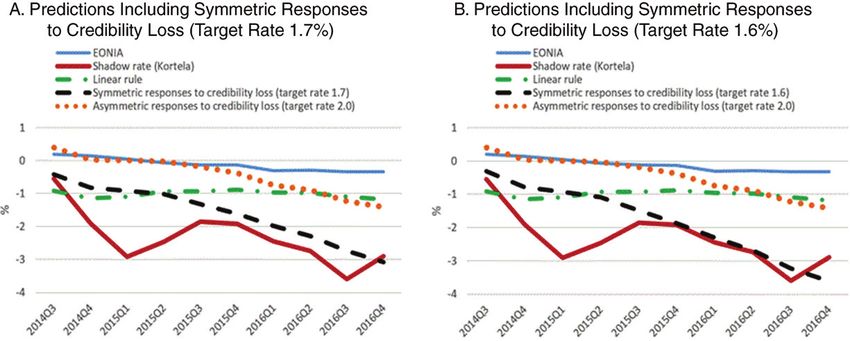
Finally, at the end of this section, we evaluate the performance
of estimated reaction functions by comparing their in-sample pre-
dictions against the key interest rates and their out-of-sample pre-
dictions against shadow interest rates estimated by Kortela (2016)
and by Wu and Xia (2016).
All estimations are based on the generalized method of moments
(GMM) with lags of regressors as instruments. We use the het-
eroskedasticity and autocorrelation corrected (HAC) (Newey and
West 1987) GMM weighting matrix, which accounts for het-
eroskedasticity and serial autocorrelation in the estimated reaction
function residuals. Use of the GMM in this context is motivated
by the potential simultaneity of the right-hand-side variables of the
reaction function. It is conceivable that the forecasts for inflation
and the cyclical variable are affected by current monetary policy.
In addition, our reaction function includes a proxy for the neutral
rate of interest, which is measured subject to error. To the extent
that these errors are correlated with other regressors, ordinary least
squares (OLS) would give biased estimates.
3.1 Linear Reaction Functions
We start with estimating a large number of competing linear reac-
tion functions, in which we use the real-time output growth gap as
a proxy for the cyclical stance in the economy:
f
it = ρit−1 + (1 − ρ)(α + βπ πt+j|t f
+ βy (yt+k|t − yt∗ ) + rt∗ ). (2)
While this reaction function is not an outcome of explicit opti-
mization based on a structural model and the central bank’s prefer-
ences, it is comparable to an inflation-forecast-targeting procedure,138 International Journal of Central Banking June 2021
advocated by Svensson and Woodford (2005), as a way to implement
optimal state-contingent policy.16
In equation (2), the MRO rate, the average EONIA rate, or
the end-of-quarter EONIA rate it measures the monetary policy
stance and the term it−1 captures interest rate smoothing. The term
f
πt+j|t refers to the ECB’s projection of j-quarters-ahead HICP infla-
f
tion and yt+k|t to the ECB’s projection of k-quarters-ahead real
GDP growth. Potential output growth (yt∗ ) is proxied by long-run
output growth projections. The underlying assumption is that the
medium-run growth projection for the euro area corresponds to the
assessed real time euro-area growth potential.17
In the original Taylor (1993) formulation, the neutral real inter-
est rate is set to a constant, equal to 2 percent. This implies together
with a 2 percent inflation target that the equilibrium nominal rate
would be 4 percent. There is compelling evidence that equilibrium
real interest rates are variable and have been trending downward
both in the United States and in the euro area recently.18 While the
16
The Eurosystem/ECB staff projections were at first based on a constant
interest rate assumption, but in order to further improve the quality and inter-
nal consistency of macroeconomic projections, both short-term and long-term
interest rate assumptions have been based on market expectations since the June
2006 projection exercise. According to the ECB (2006), “this change is of a purely
technical nature,” which “does not imply any change in the ECB’s monetary pol-
icy strategy or in the role of projections within it.” We therefore interpret this
change as if the internal forecasting procedure of the ECB had changed, but we
don’t expect a change in the reaction function itself.
17
Another option would have been to use potential output estimates. However,
the real-time estimates for euro-area potential output are only available from
2009:Q2 at a quarterly frequency and from 2006 at an annual frequency in the
ECB projection data. It is also worth noting that in the ECB’s New Area-Wide
Model (NAWM), the reaction function has been specified in terms of deviations of
output growth from its long-run empirical mean (Christoffel, Coenen, and Warne
2008).
18
Our specification of the interest rate rule, which includes a proxy for the
natural rate of interest, is akin also to Wicksell (1898), who argued that in order
to maintain price stability, monetary policy should aim to track some measure
of neutral rate determined purely by real factors (such as productivity of capi-
tal). King and Wolman (1999) and Woodford (2003) have shown that such a rule
can result from optimizing central bank behavior in a standard New Keynesian
model. In this formulation of the policy rule, when the equilibrium real rate rises,
the central bank sets the interest rate higher so as to keep the output (growth)
close to its equilibrium level (see also Cúrdia et al. 2015).Vol. 17 No. 2 What Does “Below, but Close to, 2 Percent” Mean? 139
equilibrium real interest rate is difficult to estimate and is subject
to large uncertainty, there is no reason why a time-varying equilib-
rium rate could not be incorporated into a policy rule.19 In line with
Clarida (2012) and Neuenkirch and Tillmann (2014), we append the
reaction function with the long-term real interest rate as a proxy for
the equilibrium real rate (rt∗ ). We use yields on German government
bonds of different maturities and calculate the real rate by subtract-
ing either ex ante or ex post inflation from the nominal yield.20
In order to interpret the expression “below, but close to 2 per-
cent,” we need to solve the implicit inflation target in equation
(2). Assuming that (expected) inflation is at its target level (π ∗ ),
output growth is at the potential level (yt∗ ), the natural rate is
constant (r∗ ), and the policy rate is constant over time (i), we
can present the steady-state version of equation (2) in the follow-
ing form: i = α + βπ π ∗ + r∗ . When combined with the Fisher
equation (i = π ∗ + r∗ ), we can find the implicit inflation target
π ∗ = −α/(βπ − 1).21
When estimating reaction functions, forecast horizons for
forward-looking variables are typically assumed to be relatively
short, reflecting a poorer forecast accuracy over a longer period of
time.22 However, we consider forward-lookingness of the ECB’s pol-
icy responses without fixing forecasts horizons a priori by varying
forecast horizons of inflation and output growth from zero (i.e., now-
cast) to four quarters. Correspondingly, when constructing proxies
for potential output growth, we use output growth projections from
8 to 11 quarters ahead.23
19
For discussion see, e.g., Taylor (2018).
20
Basing the proxy for the time-varying natural rate on German bunds instead
of generic GDP-weighted composite euro-area bond yields is motivated in this
context by the fact that German bund yields arguably do not contain the default
risk premiums in the latter half of the sample.
21
Since the implicit inflation target π ∗ = −α/(βπ − 1) is a ratio of estimation
coefficients, its 95 percent confidence band can be computed with the help of the
standard deviations of the coefficients α and βπ , and their correlation. Notice that
the confidence band of the implicit inflation target is typically not symmetric.
22
For example, when estimating reaction functions for the ECB, both Gerlach
and Lewis (2014) and Neuenkirch and Tillmann (2014) consider one-year-ahead
forecasts of inflation and output growth.
23
We instrument our measure of potential output growth (eight-quarters-
ahead growth forecast) with eight-quarters-ahead growth forecasts from past data140 International Journal of Central Banking June 2021
Among the resulting large number of reaction function candi-
dates, we then use the following criteria to choose our preferred
specifications in order to assess the ECB’s de facto inflation target:
(i) The computed inflation target must have a bounded 95 per-
cent confidence interval, which implies that the Taylor princi-
ple holds at the 5 percent level., i.e., βπ > 1 at the 5 percent
level. If the 95 percent confidence interval of (βπ − 1) includes
zero, the computed inflation target π ∗ = −α/(βπ − 1) does
not have a bounded confidence interval.
(ii) The 95 percent confidence interval of the inflation target
should include some values between 1.5 percent and 2.0 per-
cent. If this is not the case, we conclude that the estimated
reaction function is not consistent with the definition of price
stability and therefore it is not a good description of euro-area
monetary policy. However, we do not (automatically) exclude
models with a point estimate of π ∗ below 1.5 percent or above
2.0 percent, as long as the 95 percent confidence interval
includes some values between 1.5 percent and 2.0 percent.
(iii) We require that the estimated parameter for projected infla-
tion should be larger than that for projected real GDP
growth: βπ > βy > 0.24
We end up with 750 different specifications altogether, 13 of
which meet the selection criteria described above. Typically, these
specifications include the one-year-ahead inflation projection and
vintages. Then to instrument for the output growth gap (output growth nowcast,
or one- to four-quarters-ahead forecast – potential output growth proxy), we use
output growth nowcasts or forecasts from past data vintages (so that both ele-
ments entering the instrument for the output growth gap are from the same data
vintage). Furthermore, we also use inflation nowcasts or forecasts from past data
vintages as instruments. To be more specific, if output (inflation) forecast j = 0,
1, 2, 3, 4 periods ahead appears in the reaction function, we use the same forecast
horizon from previous data vintages as an instrument. Finally, we instrument the
nominal interest rate and the natural rate proxy with their lags. For all variables,
we have used lags 2–4. Using different lags would give similar results.
24
This is natural in the context of the ECB, as it does not have a dual man-
date like the Federal Reserve. Furthermore, even if the parameters we estimate
are not structural, also in the structural model of the euro area used at the ECB
(NAWM), the estimated reaction function has this property.Vol. 17 No. 2 What Does “Below, but Close to, 2 Percent” Mean? 141
the nowcast or one-quarter-ahead real GDP gap projection.25 In
these specifications, the ECB reacts rather strongly to projected
inflation (the point estimate of the coefficient of inflation forecast
ranges between 2.8 and 5.4, depending on specification). The reac-
tion to the GDP growth gap is considerably more muted (typically
the point estimate is roughly 0.4 or 0.5).
Figure 3 shows the computed inflation targets and their 95 per-
cent confidence intervals based on sampling uncertainty from those
seven model variants where the width of the confidence band is 100
basis points or narrower. In figure 3, the implied point estimate for
the inflation target typically lies close to 1.8 percent. In the wider
set of 13 specifications where the maximum width of the confidence
band is 200 basis points, there are also a few rules with the inflation
target at or below 1.6 percent. A rule with an inflation target of
2 percent or above is a rare exception. Furthermore, while the lower
bound of the 95 percent confidence interval can be rather low in some
rules, the upper bound typically lies below 2 percent. According to
recursive estimations, the computed inflation target is relatively sta-
ble over time, apart from the period of the financial crisis.26 In the
specifications presented in figure 4, the point estimates across the
models vary between 1.49 percent and 1.87 percent.
Finally, we augment equation (2) with the past inflation gap
term. We allow the number of lags in the inflation gap term to vary
from one to eight quarters. In this case, our preferred specification, in
which all estimated coefficients are reasonable (i.e., of the expected
sign and of meaningful size) includes the one-year-ahead inflation
forecast, GDP growth nowcast, and a natural rate proxy based on
the ex post real yield of 10-year German bunds. The monetary pol-
icy stance is measured by EONIA (average over the quarter) and the
inflation gap is based on the past six quarters. The point estimate
25
There are also five specifications which meet selection criteria (i) and (iii)
but do not meet criterion (ii). All five specifications involve the two-quarters-
ahead inflation projection. In these specifications the point estimate of the de
facto inflation target is roughly 3 percent, while the lower bound of the 95 per-
cent confidence band is typically at roughly 2.5 percent; the upper bound of the
confidence band ranges from close to 4 percent to over 10 percent, depending on
specification.
26
Estimation results are available upon request.142 International Journal of Central Banking June 2021
Figure 3. Inflation Target: Point Estimates and
95 Percent Confidence Bands
Sources: ECB and authors’ own calculations.
Notes: All specifications (1–7) displayed in the figure include the one-year-ahead
inflation projection. Specifications 1–5 also include the GDP growth nowcast,
while specification 6 includes the one-quarter-ahead, and specification 7 the two-
quarters-ahead, GDP growth forecast. In specifications 1–6, the monetary policy
stance is measured by EONIA (quarterly average), while in specification 7 the
stance is measured by the MRO rate (end of period). The natural rate of interest
is proxied by the real yield on German government bonds of different maturi-
ties: (1) five years (ex post), (2) three years (ex post), (3) two years (ex post),
(4) five years (ex ante), (5) three years (ex ante), (6) one year (ex post), and (7)
five years (ex ante).
for the de facto inflation target is π̂ ∗ = 1.77% with a 95 percent con-
fidence interval (capturing only sampling uncertainty) of 1.62–1.91
percent.27
To summarize, our estimations so far suggest that the ECB’s
monetary policy decisions are based on relatively short-term macro-
economic projections and the ECB’s de facto inflation target lies
between 1.7 percent and 1.8 percent. This finding is in line with the
analysis of the inflation forecasts in the previous section.
It is useful to compare our results with survey-based measures of
inflation expectations. Long-run inflation expectations in the ECB
Survey of Professional Forecasters are more dispersed, but their
27
Estimation results are available upon request.Vol. 17 No. 2 What Does “Below, but Close to, 2 Percent” Mean? 143
Figure 4. Recursive Expanding Window Estimations
Sources: ECB and authors’ own calculations.
Notes: The presented specification includes the four-quarters-ahead inflation
projections, output growth nowcasts, and the ex ante real natural interest rate.
The end of the estimation window is extended recursively from 2006:Q1 to
2014:Q2. Point estimates are not shown for periods for which the confidence
band isn’t bounded.
mean is comparable to our estimates of the de facto target. The
distribution of long-term point estimates reveals that inflation expec-
tations have been hovering between 1.7 and 2.0 percent during 2002–
14. When looking at the aggregate probability distribution of long-
term inflation expectations, the distribution is considerably wider
than shown in figures 3 and 4. Even if most of the probability mass
is between 1.5 and 1.9 percent, there is a considerable probability
mass also between 0.5 and 1.4 percent and between 2.0 and 2.9
percent, and even beyond (see ECB 2019).
3.2 Reaction Functions where Cyclical Variable Is Output
Growth
Measuring output gap and potential output in real time is notori-
ously difficult, and it is unlikely to be a good practice in policymak-
ing to base policy on such uncertain measures of cyclical position
of the economy. Indeed, the ECB does not discuss its output gap
measures explicitly when it communicates its policy to the public.144 International Journal of Central Banking June 2021
Consequently, it is useful to consider reaction functions which do
not directly rely on the output gap. The caveat is that the linear
specification does not allow us to infer the de facto inflation target.
However, with the inclusion of the nonlinear CL term, we can again
indirectly infer the value of the de facto inflation target without a
need to rely on an output gap measure.
3.2.1 Linear Forward-Looking Reaction Functions
For completeness, we discuss first the results from the linear speci-
fications of the following form:
f
it = ρit−1 + (1 − ρ)(α + βπ (πt+j|t − π ∗ ) + βy yt+k|t
f
+ Drtn ). (3)
f
In equation (3), it is the EONIA rate and the term πt+j|t
refers to the ECB’s projection of j-quarters-ahead HICP inflation
f
and yt+k|t to the ECB’s projection of k-quarters-ahead real GDP
growth (instead of output growth gap as in equation (2)). Both ex
ante and ex post proxies of the neutral real interest rate (rtn ) based
on the composite nominal yield of 10-year euro-area government
bonds (see figure A.2 in appendix A) are considered; when the nat-
ural real rate enters (does not enter) into a reaction function, the
dummy variable D is equal to one (zero). We set the inflation target
to a number close to 2 percent, more specifically π̂ ∗ = 1.9%.28
When estimating equation (3) with and without the natural
real interest rate proxies, we again vary projection horizons from
zero (nowcast) to four quarters.29 We estimate 75 competing spec-
ifications altogether and choose the preferred specification follow-
ing model selection criteria by which the estimated coefficients for
forward-looking variables must imply that the interest rate reacts
sufficiently strongly to projected inflation and output in order to sta-
bilize the economy, and the estimated parameter for projected infla-
tion should be larger than the one for projected real GDP growth.
28
In the NAWM model of the ECB, the operational definition of price stability
is also set at 1.9 percent (Christoffel, Coenen, and Warne 2008).
29
We employ as instruments lagged variables from the same data vintage that
is used in the monetary policy rule. We instrument inflation and output growth
forecasts and nowcasts with lags 2–5 of (realized) inflation and output growth.
As further instruments we use lags 3–4 of the nominal interest rates and lags 2–3
of the natural rate proxies. Using different lags would give similar results.Vol. 17 No. 2 What Does “Below, but Close to, 2 Percent” Mean? 145
We also assess parameter stability as well as relevance of the real
interest rate variable in the reaction function by running estimations
in which we extend the pre-crisis sample (1999:Q4–2008:Q2) recur-
sively quarter by quarter until the whole sample 1999:Q4–2014:Q2
is reached.
As in the previous section, the results support specifications with
(i) very short-run (one-quarter-ahead) GDP growth projections;
(ii) somewhat longer-term (one-year-ahead) inflation projections;
and (iii) reaction functions including a proxy for the natural rate
of interest.30
Table 1 summarizes our preferred linear specification, based
on a four-quarters-ahead inflation gap and one-quarter-ahead out-
put growth. According to this specification, the ECB reacts to a
projected inflation gap about three times stronger than to a pro-
jected cyclical stance measured by output growth. The interest rate
smoothing is rather high as expected and the relatively large coef-
ficient for the inflation gap implies that the Taylor principle clearly
holds: the real ex ante interest rate increases when inflation rises.
Inclusion of a time-varying natural rate has only a small effect on
the coefficient on output growth. The effect on the coefficient for
expected inflation gap is somewhat larger, but this difference is
partly mechanical, because we measure the real interest rate as a
difference between a composite nominal yield of 10-year euro-area
government bonds and real-time estimates of the current or one-
period-ahead inflation forecast. Overall, it seems reasonable that the
ECB conditions its interest rate decisions on the short end of the
30
We obtain statistically significant coefficients also for the nowcast as well as
one-quarter-ahead or four-quarters-ahead inflation, if the forecast horizon for real
GDP growth is very short, i.e., zero (nowcast) or one quarter. Notably, a speci-
fication with the four-quarters-ahead inflation and one-quarter-ahead real GDP
f
growth (i.e., πt+4|t and yt+1|t
f
) produces satisfactory coefficient estimates with
either of the two proxies of the natural real interest rate, as well as without a nat-
ural rate proxy. Regarding parameter stability, we have estimated reaction func-
f
tions with the four-quarters-ahead inflation (πt+4|t ) and one-quarter-ahead GDP
f
(yt+1|t ) for the (pre-Lehman) period of 1999:Q4–2008:Q2, and then expanded
the sample one quarter at a time until 2014:Q2. We obtain more stable coeffi-
cients for inflation and output growth with a natural interest rate proxy in the
specification than without it. In addition, the specification using the ex ante nat-
ural real interest rate seems to work even better than the ex post natural real
interest rate. All results are available upon request.146 International Journal of Central Banking June 2021
Table 1. Baseline Linear Reaction Function with Output
Growth as Cyclical Variable
it = ρ ∗ it−1 + (1 − ρ) ∗ (α + βπ ∗ (πt+4|t
f
− 1.9) + βy ∗ Δyt+1|t
f
+ r̃t10yr )
Coefficient Std. Error t-statistic Prob.
ρ 0.84 0.044 19.23 0.0000
α −0.95 0.737 −1.29 0.2049
βπ 4.45 0.832 5.34 0.0000
βy 1.48 0.507 2.92 0.0057
J-statistic 6.07
Prob(J-statistic) 0.73
Notes: This table shows the GMM estimation results of our preferred linear reac-
tion function of the ECB. The estimation sample is 1999:Q4–2014:Q2. See the main
text for the definition of the variables and table B.1 (in appendix B) for alternative
competing linear specifications. The reported J-statistic is the Sargent-Hansen test
for validity of the instruments.
forecast horizon due to increasing difficulties to predict inflation and
growth in the medium and longer term.
3.2.2 Symmetric Responses to Past Inflation Gaps
Next, we augment our preferred linear specification with a backward-
looking “credibility loss term” CLt so that
f
it = ρit−1 + (1 − ρ)(α + βπ (πt+4|t − π∗)
f
+ βy yt+1|t + γCLt + rtn ), (4)
where the CLt term is specified as in equation (1).
As discussed at the beginning of this section, this term captures
the idea that the central bank may set the interest rate higher (lower)
today if the past inflation gap is positive (negative) even if inflation
is projected to be at the target in the near future.31,32 Concerns for
31
Monetary policy credibility measures proposed by de Mendonca and de
Guimarães e Souza (2009) is also based on past deviations of inflation from the
target.
32
Using quite similar an approach, Dovern and Kenny (2017) investigate the
impacts of “too low for too long” on long-term inflation expectations of profes-
sional forecasters in the euro area. They define an inflation “performance gap”Vol. 17 No. 2 What Does “Below, but Close to, 2 Percent” Mean? 147
past inflation gaps may reflect, e.g., the central bank’s desire and
commitment to correct past errors. Note also that the credibility
loss term weights large average past deviations of inflation from the
target (π ∗ ) more than small ones. Note that in Bernanke’s (2017b)
proposal of temporary price-level targeting, the key additional ele-
ment in the policy rule is the term which captures the cumulative
inflation shortfall since the beginning of zero lower bound until the
exit date (see also Hebden and López-Salido 2018). The CL term
captures a similar idea, but it introduces additional inertia in pol-
icymaking also at normal times when inflation deviates from the
target.
When estimating equation (4), we allow for the length of the
time span, i.e., the number of lags (q) over which the average past
inflation is measured, to vary from one to eight quarters.33 We
also consider a number of different inflation targets π ∗ , at or below
2 percent; the lowest inflation target rate examined is chosen to be
1.6 percent in light of figure 1 and the results from section 3.1. This
exercise allows us to draw additional indirect inference concerning
both the ECB’s de facto inflation target and the ECB’s concerns of
past inflation gaps.
Estimation results are summarized in table B.2 in appendix B.
Based on our model evaluation criteria, longer credibility loss time
spans, ranging up to six to eight lags, and lower inflation target
rates (perhaps even as low as 1.6 percent or 1.7 percent) produce
the most satisfactory and relatively robust coefficient estimates (esti-
mated parameters seem to be relatively stable when the sample rolls
recursively over the financial crisis toward 2014:Q234 ). Our preferred
nonlinear specification is reported in table 2. Compared with the
linear specification in table 1, we now obtain smaller coefficients for
interest rate smoothing and projected inflation gap while the ECB
seems to react relatively strongly to past inflation gaps. The esti-
mated output growth coefficient is roughly unchanged relative to
the preferred linear specification.
as the difference between recent long-term inflation expectations and a moving
average of past inflation rates.
33
We do not instrument for the CL terms (which include past values of infla-
tion), while the rest of the right-hand-side variables are instrumented as explained
in section 3.2.1.
34
The results are available upon request.148 International Journal of Central Banking June 2021
Table 2. Baseline Reaction Function with Symmetric
Response to Past Inflation Gap
it = ρ ∗ it−1 + (1 − ρ) ∗ (α + βπ ∗ (πt+4|t
f
− 1.7) + βy ∗ Δyt+1|t
f
+ γ ∗ CLt + r̃t10yr ) where CLt = (π̄t−1,t−7 − 1.7)|π̄t−1,t−7 − 1.7|
Coefficient Std. Error t-statistic Prob.
ρ 0.77 0.051 15.30 0.0000
α −1.51 0.396 −3.83 0.0004
βπ 3.61 0.798 4.53 0.0001
βy 1.25 0.317 3.94 0.0013
γ 1.07 0.417 2.56 0.0145
J-statistic 6.58
Prob(J-statistic) 0.68
Notes: This table shows the GMM estimation results of our preferred reaction func-
tion of the ECB including symmetric reactions to past inflation gaps. The estimation
sample is 1999:Q4–2014:Q2. See the main text for the definition of the variables
and table B.2 (in appendix B) for alternative competing linear specifications. The
reported J-statistic is the Sargent-Hansen test for validity of the instruments.
In sum, we find that a concern for past errors seems to have
played a role in the ECB’s policy decisions. Quite intuitively, how-
ever, the ECB has responded only to persistent inflation gaps as
indicated by the long lags of the credibility loss term.35 Consistently
with the findings from section 3.1, these results also suggest that the
ECB’s de facto inflation target has been considerably below 2 per-
cent, perhaps even as low as 1.6 percent or 1.7 percent.36 Hence,
the results for the de facto inflation target do not seem to be overly
sensitive to the choice of the cyclical variable or even the inclusion
of the past inflation gap term.37
35
This is reasonable, since monetary policy is not expected to respond to
temporary shocks to inflation such as large variations in energy prices.
36
Bletzinger and Wieland (2017), using the ECB Survey of Professional Fore-
casters and European Commission estimates for potential growth, and consid-
ering a target range of 1.5–2.0 percent, conclude that the ECB point inflation
target is 1.7 percent. Furthermore, when estimating first-difference policy rules
by Orphanides (2003), Hartmann and Smets (2018) conclude that the ECB’s
implicit target is 1.81 percent.
37
As a further robustness check, we have also estimated a number of linear reac-
tion functions without any real activity measure. These specifications are basedVol. 17 No. 2 What Does “Below, but Close to, 2 Percent” Mean? 149
3.2.3 Asymmetric Responses to Past Inflation Gaps
Next, we consider possible asymmetry in the ECB’s policymaking,
i.e., we allow for different responses to positive and negative past
inflation gaps. We estimate the following specification:
f
it = ρ ∗ it−1 + (1 − ρ) ∗ (α + βπ ∗ (πt+4|t − π ∗ ) + βy ∗ yt+1|t
f
−
+ γ1 ∗ CL+
t + γ2 ∗ CLt + rt ),
n
(5)
where
CL+ CL
t = Dt ∗ CLt
CL−
t = (1 − Dt ) ∗ CLt .
CL
In equation (5), the dummy variable DtCL is equal to one (zero)
if CLt > 0 (CLt < 0). The coefficient γ1 captures monetary policy
reactions to past positive inflation gaps, and the coefficient γ2 to
past negative inflation gaps. In order to measure the ECB’s credi-
bility concerns in a meaningful way, the parameters γ1 and γ2 must
be positive, but their sizes may differ.
Again, we run several competing specifications in order to draw
some inference concerning both the ECB’s de facto inflation tar-
get and the ECB’s concerns of past inflation gaps. In table B.3 in
appendix B, the credibility loss term is based on one to eight lags
of actual inflation and the inflation target varies from 1.6 to 2.0
percent. Consistent with our results for symmetric reaction func-
tions, table B.3 in appendix B indicates that the time span of the
past inflation gap should be rather long, ranging from six to eight
quarters (the ECB reacts only to rather persistent inflation gaps).
However, as our preferred specification in table 3 reveals, now the
inflation target closer to 2 percent seems more appropriate but the
ECB’s policy is asymmetric: it responds more aggressively to pos-
itive than to negative inflation gaps (i.e., the parameter estimate
for γ1 is significantly larger than for γ2 ).38 Such an asymmetric
on the assumption that the ECB policy responds only to projected inflation. The
results are not sensitive to the inclusion or exclusion of a cyclical variable.
38
Note that a time-invariant potential output can be calculated as y ∗ =
(π ∗ − α)/βy . According to the symmetric reaction function (asymmetric reac-
tion function), the average projected potential output growth is 2.5 percentYou can also read