Feshbach-Fano approach for calculation of Auger decay rates using equation-of- motion coupled-cluster wave functions. I. Theory and implementation
←
→
Page content transcription
If your browser does not render page correctly, please read the page content below

Feshbach–Fano approach for calculation
of Auger decay rates using equation-of-
motion coupled-cluster wave functions. I.
Theory and implementation
Cite as: J. Chem. Phys. 154, 084124 (2021); https://doi.org/10.1063/5.0036976
Submitted: 09 November 2020 . Accepted: 21 January 2021 . Published Online: 26 February 2021

  Wojciech Skomorowski, and        Anna I. Krylov

J. Chem. Phys. 154, 084124 (2021); https://doi.org/10.1063/5.0036976                     154, 084124

© 2021 Author(s).
The Journal
ARTICLE scitation.org/journal/jcp
of Chemical Physics
Feshbach–Fano approach for calculation
of Auger decay rates using equation-of-motion
coupled-cluster wave functions. I. Theory
and implementation
Cite as: J. Chem. Phys. 154, 084124 (2021); doi: 10.1063/5.0036976
Submitted: 9 November 2020 • Accepted: 21 January 2021 •
Published Online: 26 February 2021
Wojciech Skomorowskia) and Anna I. Krylova)
AFFILIATIONS
Department of Chemistry, University of Southern California, Los Angeles, California 90089, USA
a)
Authors to whom correspondence should be addressed: skomorow@usc.edu and krylov@usc.edu
ABSTRACT
X-ray absorption creates electron vacancies in the core shell. These highly excited states often relax by Auger decay—an autoionization
process in which one valence electron fills the core hole and another valence electron is ejected into the ionization continuum. Despite
the important role of Auger processes in many experimental settings, their first-principles modeling is challenging, even for small sys-
tems. The difficulty stems from the need to describe many-electron continuum (unbound) states, which cannot be tackled with standard
quantum-chemistry methods. We present a novel approach to calculate Auger decay rates by combining Feshbach–Fano resonance the-
ory with the equation-of-motion coupled-cluster single double (EOM-CCSD) framework. We use the core–valence separation scheme
to define projectors into the bound (square-integrable) and unbound (continuum) subspaces of the full function space. The contin-
uum many-body decay states are represented by products of an appropriate EOM-CCSD state and a free-electron state, described by
a continuum orbital. The Auger rates are expressed in terms of reduced quantities, two-body Dyson amplitudes (objects analogous to
the two-particle transition density matrix), contracted with two-electron bound-continuum integrals. Here, we consider two approxi-
mate treatments of the free electron: a plane wave and a Coulomb wave with an effective charge, which allow us to evaluate all req-
uisite integrals analytically; however, the theory can be extended to incorporate a more sophisticated description of the continuum
orbital.
Published under license by AIP Publishing. https://doi.org/10.1063/5.0036976., s
I. INTRODUCTION ionized liquid water,10,11 a photo-induced ring-opening reaction,12
and charge-migration and charge-transfer reactions13–15 and to
Owing to their ability to target specific atomic sites while interrogate the interplay between open-shell spin-coupling and
being sensitive to the chemical environment, core-level spectro- Jahn–Teller distortion in the benzene radical cation.16,17
scopies are powerful tools for interrogating the molecular struc- Absorption of an x-ray photon, creating a vacancy in the core
ture.1–3 The underlying versatile selection rules governing excitation shell, leaves the molecule in a highly excited state. In molecules
processes to the excited states in either the bound or the contin- composed of light atoms (such as C, N, or O), these core-level
uum part of the spectrum enable a broad range of applications. states decay predominantly through a non-radiative autoionization
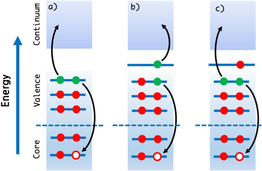
Advances in laser technology and the development of novel x-ray process called Auger decay.18 In this process, shown schematically
sources have opened up a new area of applications in which core- in Fig. 1, the core hole is filled with an electron from a valence
level spectroscopies can be used as probes to study electron and orbital, liberating sufficient energy to eject another valence electron
nuclear dynamics with unprecedented time and space resolution.4–9 (called an Auger electron) into the continuum. Having characteristic
Recently, x-ray spectroscopy was used to reveal the dynamics of timescale on the order of femtoseconds, Auger processes compete
J. Chem. Phys. 154, 084124 (2021); doi: 10.1063/5.0036976 154, 084124-1
Published under license by AIP Publishing
The Journal
                                                                                                                        ARTICLE                scitation.org/journal/jcp
 of Chemical Physics

                                                                                                 FIG. 2. In the Feshbach–Fano framework, a resonance state is described in terms
                                                                                                 of the interaction between bound and continuum states. The two domains are
                                                                                                 defined by means of the Feshbach projection operators, Q and P, which split the
                                                                                                 total Hamiltonian into the bound (shown by the green solid curve) and unbound
                                                                                                 (shown by the red solid curve) parts. The resonance state is described by a bound
                                                                                                 eigenstate from the Q subspace (shown in green) coupled to the continuum states
                                                                                                 from the P subspace (shown in red). As a result of this mixing, the total wave func-
                                                                                                 tion of the resonance (light blue solid curve) has two distinguishable components:
                                                                                                 the bound-like (in the interaction region) and the scattering-like (in the asymptotic
      FIG. 1. Different types of Auger effect: (a) regular Auger decay, (b) resonant (partic-    region).
      ipator) decay, and (c) resonant (spectator) decay. Regular Auger decay is relevant
      for x-ray photoionization spectroscopy (XPS), whereas resonant Auger processes
      occur in x-ray absorption spectroscopy (XAS).

                                                                                                our theoretical framework. Feshbach projection operators Q and
                                                                                                P divide the full function space into the bound and continuum
    directly with electron and nuclear dynamics triggered by prior x-                           domains. Similar to Fano’s picture, in Feshbach’s construction, the
    ray photon absorption. Auger decay also plays an important role in                          resonance state is described as a bound state from the discrete sub-
    molecular imaging using ultrashort x-ray pulses from free-electron                          space Q coupled to the continuum subspace P. By using the parti-
    lasers, where it contributes to the damage of the sample, limiting                          tioning technique,29,30 the Schrödinger equation can be mapped into
    the achievable resolution.19,20 By measuring the kinetic energy of the                      an eigenproblem in the Q-space with an effective Hamiltonian incor-
    emitted electron, Auger electron spectroscopy is used in studies of                         porating the P-space. Most often, one treats the bound part of the
    surfaces, materials, nanostructures, and gas-phase molecules.21–24                          Hamiltonian and the respective eigenstates as zero-order states and
          The first theoretical description of Auger decay was due to                           includes the effect of the continuum at the first-order perturbation,
    Wentzel, who employed a perturbative approach to calculate transi-                          as was done in the original paper of Feshbach.28 The critical aspect
    tion rates into the continuum in an atom with two active electrons.25                       of the Feshbach–Fano formalism is that the quality of the results
    The key assumption was that Auger decay is a two-step process                               depends strongly on the choice of the projector operators, which are
    in which the emission of the Auger electron is independent of the                           not rigorously defined. This is the main stumbling block for quan-
    preceding core–shell depletion created by means of x-ray photoion-                          titative applications of the Feshbach–Fano formalism to many-body
    ization or absorption transition. Hence, the initial state for the Auger                    autoionization problems. Among recent attempts to develop physi-
    decay can be treated as an electronically metastable state, undergoing                      cally and theoretically justified projectors, the works of Martin and
    spontaneous ionization.                                                                     co-workers31 and Kunitsa and Bravaya32 are notable.
          Multichannel resonance scattering theory18,26 provides an alter-                            Fortunately, in the case of Auger decay, one can easily sep-
    native, more-sophisticated treatment of autoionization, including                           arate the bound and continuum many-body configurations in the
    the Auger effect. In this framework, the autoionizing state appears                         Fock space. This is possible because (i) the core-level states are Fes-
    as a pole in the scattering matrix for complex-valued electron colli-                       hbach resonances, which can only decay by a two-electron process,
    sion energy. The scattering wave function in the vicinity of an iso-                        and (ii) the core orbitals are well separated from the valence orbitals.
    lated resonance state can be decomposed into two parts: bound-like                          Thus, Slater determinants, in which at least one core orbital is active,
    and continuum-like. The former is square-integrable, and it closely                         form the bound domain, which can only couple to the continuum
    resembles a regular bound state, whereas the latter is non-square                           by pure valence excited determinants. This is exploited in the core–
    integrable and fully determines the asymptotic behavior of the                              valence separation (CVS)33 scheme commonly used to adapt stan-
    state.                                                                                      dard electronic structure methods for treating core-level states.34–43
          Such a decomposition of the wave function is the essence of the                       The CVS ansatz decouples core-excited and core-ionized states from
    Feshbach–Fano approach27,28 for treating autoionizing states (res-                          the valence continua, essentially acting as the Feshbach Q projec-
    onances). As originally formulated by Fano27 and shown in Fig. 2,                           tor. In standard applications of the CVS scheme, the continuum is
    the autoionization can be described in terms of mixing between                              simply ignored, and the core-level states are treated as bound states
    discrete and continuum diabatic electronic states, coupled by the                           (in terms of perturbation theory, one can think of these CVS states
    off-diagonal (i.e., continuum-bound) matrix elements of the many-                           as zero-order states). Here, we extend the theory and include the
    body Hamiltonian. Feshbach put this idea on a more rigorous                                 effect of the continuum by explicitly constructing the decay states
    mathematical basis by using projector operators and the partition-                          and evaluating the matrix elements between the bound and contin-
    ing approach,28 known in the quantum chemistry community as                                 uum many-body states. In this way, we obtain first-order corrections
    the Löwdin partitioning technique.29 This approach is the basis of                          to the energies of the core-level states: the real part of the correction

J. Chem. Phys. 154, 084124 (2021); doi: 10.1063/5.0036976                                                                                                                 154, 084124-2
Published under license by AIP Publishing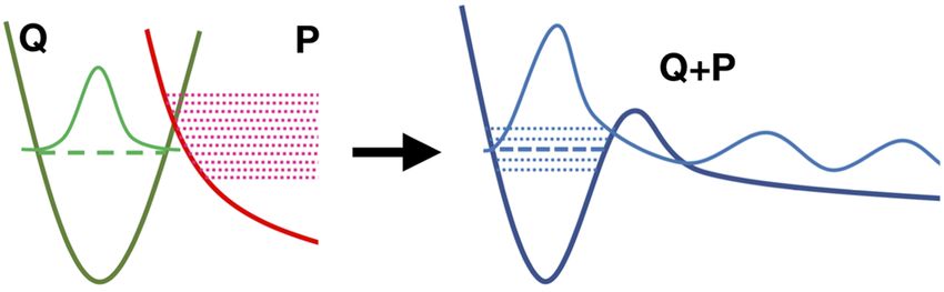
The Journal
                                                                                                  ARTICLE            scitation.org/journal/jcp
 of Chemical Physics

    adjusts the position of the resonance and the imaginary part gives its    elaborate calculations of the Auger widths can be carried out with
    width.                                                                    the multi-configurational Dirac–Fock method implemented in the
          The construction of the many-body decay states poses greater        RATIP program.68 However, the results depend strongly on the
    difficulties for the theory than the construction of the initial states   manual selection of configurations included in the subspace for the
    (which can be treated by CVS) because the decay states belong             initial and final states. For molecules, the most advanced method
    to the continuum (Feshbach P subspace) and cannot be properly             today is the Fano–ADC–Stieltjes approach.55,57 The drawbacks of
    represented with L2 -integrable functions used in electronic struc-       this approach are that it requires large, non-standard orbital basis
    ture calculations. The inherent difficulty in treating unbound many-      sets and that it relies on somewhat arbitrary division of the elec-
    electron systems44–47 is the reason why calculations of the Auger         tronic configurations into bound and continuum subspaces. Clearly,
    decay rates are still not routine, even for small molecules. The exist-   there is a need for more-universal computational tools for reliable
    ing approaches can be divided into three categories: (i) methods that     treatment of Auger decay. Ideally, such new computational proto-
    do not consider the state of the emitted Auger electron, (ii) methods     cols should be cost-effective, easy to set up, and take advantage of
    that treat the Auger electron implicitly without the continuum func-      the already available, highly accurate methods and algorithms of
    tions, and (iii) methods that describe the Auger electron explicitly      standard quantum chemistry.
    with a true continuum orbital.                                                  Here, we propose a methodology to calculate Auger decay
          The first category includes electron population analysis,48 in      rates based on equation-of-motion coupled cluster (EOM-CC) the-
    which the relative Auger rates are computed from the densities of         ory.69–72 We use EOM-CC to describe the bound part of the wave
    the valence molecular orbitals on the atom with the core hole. In         function in the initial and final states of the Auger decay and use
    a similar spirit, statistical approaches estimate Auger spectra from      continuum orbitals to represent the Auger electrons. The EOM-
    the distribution of final products of the decay and their decomposi-      CC framework provides effective and robust tools for computing
    tion in terms of the weights of electronic configurations.49,50 These     energies and properties of excited, ionized, and electron-attached
    methods are useful for larger systems with high density of the final      states.69–72 The flexibility of the EOM-CC single-reference ansatz
    states.                                                                   allows one to tackle states of open-shell73 and multi-configurational
          The second category comprises methods that treat the many-          character74,75 with high and controllable accuracy. EOM-CC meth-
    electron continuum states implicitly, by means of L2 -integrable          ods have been combined with complex absorbing potentials to study
    wave functions. This is done in the Green’s operator formal-              properties of metastable states.47,76,77 To enable access to core-level
    ism,51 non-Hermitian theories such as the complex absorbing               states, EOM-CC methods have been combined with CVS,33 result-
    potential approach,52 or in the Stieltjes imaging procedure.53,54         ing in a highly effective CVS-EOM-CC scheme. The CVS-EOM-
    Stieltjes imaging entails calculations of bound–continuum cou-            CCSD approach has been used to compute energies and properties
    plings by using a discretized representation of the continuum             of core-ionized and core-excited states, as well as x-ray non-linear
    by an L2 -integrable basis set. This approach has been com-               properties such as resonant inelastic x-ray scattering (RIXS).34–39,42,78
    bined with the algebraic diagrammatic construction (ADC) within           We note that the core-level spectra can also be described by the
    the Fano ansatz to compute Auger rates in atoms and small                 time-dependent coupled-cluster treatment without invoking the
    molecules.55–57                                                           CVS scheme, as was recently demonstrated by Park et al.79 In this
          In the third category of methods, the continuum character of        work, the full electronic spectrum was obtained from both time-
    the Auger electron is treated explicitly. The wave function for the       propagation of the ground-state wave function and by diagonalizing
    final state is represented by an antisymmetrized product of a func-       the time-independent Hamiltonian. The authors also showed that a
    tion for the bound molecular ion and a continuum orbital for the          systematic inclusion of different effects (higher excitations and basis
    outgoing electron. In the early days, the bound ion was treated at        sets) within the EOM-CC framework results in a sub-eV accuracy in
    the self-consistent mean-field level.58,59 More recently, various fla-    computed absolute core-excitation energies.79
    vors of configuration interaction (CI) methods have been employed               In the present work, we extend the EOM-CC methodology
    to calculate the bound part of the multi-electron wave function.60–63     to describe the autoionization properties of core-ionized and core-
    The continuum orbital for each decay channel can be computed              excited states. We combine many-electronic states described by
    using a single-center expansion method and performing numerical           CVS-EOM-CCSD with a continuum orbital, which we approximate
    integration of the effective one-electron Schrödinger equation with       by a plane wave or a Coulomb wave. This obviates numerical inte-
    proper scattering boundary conditions.64 These approaches have            gration in the calculations of mixed bound-continuum electron-
    been shown to yield accurate results for Auger spectra of small sys-      repulsion integrals. The working equations for the calculations of
    tems such as Ne and H2 O.60,62 For molecules, a one-center approxi-       the partial autoionization widths are expressed in terms of one- and
    mation is commonly employed, where it is assumed that the contin-         two-body Dyson functions, contracted with the bound-continuum
    uum orbital has the same form as in an atom bearing the core hole         integrals. While Dyson orbitals have been utilized in the theory of
    and relevant two-electron integrals have contributions only from          one-photon photoionization,80–87 here, we extend this concept
    the orbitals centered on that atom.59,65 This approach is employed,       to two-body functions, which enable a compact representation
    for example, in the XMOLECULE package for modeling ultrafast              of autoionization widths obtained from correlated many-electron
    dynamics in strong fields.66,67                                           states. In this paper, we describe the theoretical approach and its
          Although quite a few methods and algorithms for calcula-            implementation in an electronic structure code. In Paper II,88 we
    tions of Auger spectra have been reported so far, their scope of          illustrate the performance of the theory by simulating normal and
    applicability remains limited and their predictive power depends          resonant Auger decay spectra in a set of benchmark atomic and
    on the underlying ab initio method. For example, for atoms,               molecular systems, including Ne, H2 O, CH4 , and CO2 .

J. Chem. Phys. 154, 084124 (2021); doi: 10.1063/5.0036976                                                                                  154, 084124-3
Published under license by AIP Publishing
The Journal
ARTICLE scitation.org/journal/jcp
of Chemical Physics
II. FESHBACH–FANO–LÖWDIN FRAMEWORK HPP = HPP + HPQ GQ (E)HQP , (7)
As outlined above, our treatment of the autoionization pro-
HQQ = HQQ + HQP GP (E)HPQ ,
(+)
cess is based on the concepts originally formulated by Feshbach to (8)
describe nuclear reactions.28 This is an application of the Löwdin
partitioning technique29 to treat the bound-continuum problem.
(+)
where GQ and GP are the Green’s functions in the Q- and P-spaces,
While the focus of this paper is on the Auger effect, the theory is
general and can be applied to other resonance phenomena.32 GQ (E) =
1
, (9)
Let us start by reviewing the key concepts of the approach. The E − HQQ
principal idea28,29 is the introduction of two Hermitian, mutually
orthogonal, projection operators Q and P such that (+) 1
GP (E) = lim . (10)
ε→0 E + iε − HPP
Q + P = 1, QP = PQ = 0. (1)
Both HPP and HQQ are energy-dependent and non-local.30 They act
The operators Q and P divide the full function space into two sub- only in their respective subspaces; yet, due to the presence of the
spaces: the Q-space, characterizing the interaction region with the coupling H PQ/QP , they also include the effect of the complementary
discrete spectrum, and the P-space, characterizing the asymptotic subspace. Although they appear equivalent, the HPP and HQQ effec-
region with the continuous spectrum. The projection operators can tive Hamiltonians have different properties and applications. HPP is
be expressed as sufficient to obtain the asymptotic form of the total wave function,
∞ Eq. (5), and, thus, to calculate all scattering properties of the system.
By construction, the effective Hamiltonian HQQ is non-
± ±
Q = ∑ ∣ψn ⟩⟨ψn ∣, P = ∑ ∫ dE∣χμ,E ⟩⟨χμ,E ∣, (2)
n μ 0
Hermitian and has complex eigenvalues. These eigenvalues are not
equal to the eigenvalues of the original Hamiltonian, Eq. (5), solved
where the representing functions are the eigenstates of the respective
with normal boundary conditions. Rather, they represent the solu-
projected Hamiltonians,
tion of the original problem with outgoing wave boundary con-
±
HQQ ψn = En ψn , HPP χμ,E ±
= (E + Eμ )χμ,E , (3) ditions, as in the Siegert treatment.89 This property of the Fesh-
bach solutions results from the use of the G+P Green’s operator. The
with H QQ ≡ QHQ and H PP ≡ PHP. H is the total electronic Hamil- Feshbach–Fano treatment is closely related to other incarnations
tonian of the system, explicitly given in Sec. III. These functions are of the non-Hermitian quantum mechanics46 designed to describe
subject to the following normalization conditions: resonance states by using an L2 representation of the wave function.
Indeed, if the P and Q operators are defined in an adequate way,
±
⟨ψn ∣ψk ⟩ = δnk , ⟨χμ,E ∣χμ±′ ,E′ ⟩ = δμμ′ δ(E − E′ ). (4) then the eigenstates of HQQ
Thus, functions forming the Q-space are L2 -normalized, whereas HQQ ψ̃n = E˜n ψ̃n , (11)
the P-space comprises scattering (unbound) states with Dirac’s δ
normalization. For the unbound states χμ,E±
, the index μ denotes a can be identified with true resonances and their respective eigenval-
distinct open channel and the superscript ± refers to either outgoing ues
or incoming asymptotic boundary conditions imposed on the scat- Γn
E˜n = En − i (12)
tering wave function. In Eq. (3), we introduced Eμ , which denotes 2
the threshold energy of a given channel, i.e., Eμ corresponds to the correspond to physical observables, i.e., the position (En ) and the
internal energies of the two subsystems formed after the break-up. width (Γn ) of the resonance.
Similar to the Fano picture,27 a resonance in the Feshbach theory As in the context of electron correlation, the exact solution of
can be seen as an isolated bound state from the Q-space, interacting HQQ is impractical. Instead, perturbation theory can be employed,
with a bath of continuum states from the P-space. This interaction taking H QQ as the zero-order Hamiltonian and treating the rest as
(or coupling) is responsible for the decay of the resonance. For this a perturbation.30,90–92 Thus, the eigenstates of H QQ are zero-order
construction to be valid, the operator P must include the summa- wave-functions,
tion over all possible open channels μ contributing to the decay of
HQQ ψn = En ψn , (13)
the given resonant state.
The Q and P operators transform the full Schrödinger equation and En is zero-order energy of the resonance (because H QQ is Her-
HΨ = EΨ (5) mitian, and En is real). The first-order correction to the energy is
then
into an equivalent set of two sets of coupled equations, represented (1)
En
(+)
= ⟨ψn ∣HQP GP HPQ ∣ψn ⟩. (14)
as
By using the distribution property,
H H QΨ QΨ
[ QQ QP ][ ] = E[ ], (6)
HPQ HPP PΨ PΨ 1 1
lim = P.V. ∓ iπδ(x), (15)
ε→0 x ± iε x
where H PQ ≡ PHQ and H QP ≡ QHP. These two equations can be
rearranged to define two effective Hamiltonians, HPP and HQQ , we arrive at the following expressions for the resonance position:
J. Chem. Phys. 154, 084124 (2021); doi: 10.1063/5.0036976 154, 084124-4
Published under license by AIP PublishingThe Journal
ARTICLE scitation.org/journal/jcp
of Chemical Physics
En = Re⟨ψn ∣HQQ ∣ψn ⟩ = En + Δn = En where Eμ is the energy of the stable ion. Constants cα and cβ are
∞ ±
⟨ψn ∣HQP ∣χμ,E ±
⟩⟨χμ,E ∣HPQ ∣ψn ⟩ determined by spin adaptation and are expressed in terms of the
+ ∑ P.V. ∫ dE Clebsch–Gordan coefficients as
μ 0 En − Eμ − E
1 1 1
≡ En + ∑ Δμ,n , (16) cα = ⟨ , ; S′, MS − ∣S, MS ⟩,
μ 2 2 2
and for the resonance width,
1 1 1
cβ = ⟨ , − ; S′, MS + ∣S, MS ⟩.
Γn = −2Im⟨ψn ∣HQQ ∣ψn ⟩ 2 2 2
± ±
= ∑ 2π⟨ψn ∣HQP ∣χμ,E n −Eμ
⟩⟨χμ,E n −Eμ
∣HPQ ∣ψn ⟩ In this way, the final continuum state χ has the same total spin S as
μ the initial state, which is a consequence of the spin conservation in
≡ ∑ Γμ,n , (17) the course of auto-ionization. From the angular momentum algebra,
μ we know that possible spins of the final ion states are S′ = S ± 21 .
Without loss of generality, we can assume that the initial state has
in the first order of the perturbation theory. The second term in non-negative spin projection, i.e., M S ≥ 0, and in the following, we
Eq. (16) represents a shift in the position of the resonance due to consider the continuum state in the simplified form as
the coupling with the continuum. Both the energy shift Δn and
the width Γn are sums over partial contributions from each open ∣χμ,E ⟩ = â†k,α ∣S ,MS − 2 ΨN−1
′ 1
⟩, (21)
μ
channel μ.
We note that this treatment is meaningful only if ψ n provides a
where there is only one component with α spin of the free elec-
good approximation to the resonance wave-function and the pertur-
tron. To account for the properly spin-adapted form of χ, Eq. (19), a
bation does not change its character. In other words, this treatment
degeneracy factor defined as
is justified for isolated, non-overlapping resonances. The coupling
Hamiltonian H QP/PQ can be represented as H QP/PQ = H − H 0 , where 1
H 0 is a part of the total Hamiltonian H (which does not couple Q- gα = (22)
± cα2
and P-spaces) and both ψ n and χμ,E n −Eμ
are eigenstates of H 0 with the
same eigenvalue En . is included in the final expressions for the partial widths Γn,μ and
energy shifts Δn,μ . Thus, from now on, we assume that the Auger
III. AUGER TRANSITION AMPLITUDES electron has spin α and drop all spin quantum numbers in states’
AND ONE- AND TWO-BODY DYSON FUNCTIONS labels as they only enter the final expressions via the degeneracy
factor g α .
We now discuss how to generate bound and continuum zero- In what follows, we assume the strong orthogonality condition
order electronic states within the EOM-CC framework and how to —that is, that the continuum orbital corresponding to the opera-
effectively compute the transition amplitudes ⟨ψ n |H QP |χ μ,E ⟩ = ⟨ψ n |H tor âk is orthogonal to all orbitals from the bound domain present
− En |χ μ,E ⟩ entering the expressions for the partial widths and energy in ∣ΨNn ⟩ or ∣ΨμN−1 ⟩ states. This “killer condition” can be formally
shifts. Our derivation follows, to some extent, the work of Manne expressed as
and Ågren,93 who derived general expressions for the Auger ampli-
tudes from the many-electron wave function, with the adjustments âk ∣ΨNn ⟩ = âk ∣ΨN−1 ⟩ = 0, ⟨ΨNn ∣â†k = ⟨ΨN−1 ∣â†k = 0. (23)
μ μ
to accommodate coupled-cluster theory and our assumption about
the continuum orbital. We denote the initial (bound) state from the In the derivation of transition amplitudes, we express the Hamilto-
Q-space as nian in the second quantization form,
∣ψn ⟩ = ∣S,MS ΨNn ⟩, (18)
† 1 † †
where S and M S are spin quantum numbers and the superscript N H = Ô1 + Ô2 = ∫
∑ hpq âp âq + ∫∑ gpqrs âp âq âs âr , (24)
pq 2 pqrs
is the number of electrons. The final (continuum) states of the N-
electron system after the autoionization can be represented as where hpq denotes the one-electron integrals (kinetic energy and
nuclear–electron interaction), g pqrs denotes electron-repulsion inte-
∣χμ,E ⟩ = cα â†k,α ∣S ,MS − 21
⟩ + cβ â†k,β ∣S ,MS + 21
′ ′
ΨN−1
μ ΨN−1
μ ⟩, (19) grals ⟨pq|rs⟩, and the symbol ∑ ∫ signifies that this summa-
tion includes spin-orbitals from both the bound and continuum
where ∣S ,MS − 2 ΨNμ − 1 ⟩ denotes a stable, N − 1 electron core and â†k,σ
′ 1
domains. The creation and annihilation operators fulfill the anti-
2 commutation relation,
are creation operators of the free electron of energy E = k2 and spin
σ. If the initial resonant state has energy En , then the energy of the â†p âq + âq â†p = δpq . (25)
ejected electron fulfills the following condition (in atomic units):
By employing strong orthogonality and using anti-commutation
k2 properties, the one-electron part of the right transition amplitude
En = + Eμ , (20)
2 assumes the following form:
J. Chem. Phys. 154, 084124 (2021); doi: 10.1063/5.0036976 154, 084124-5
Published under license by AIP PublishingThe Journal
ARTICLE scitation.org/journal/jcp
of Chemical Physics
√
⟨ΨNn ∣Ô1 ∣ â†k ΨN−1 ⟩ = ⟨ ΨNn ∣∫ † † N−1
∑ hpq âp âq âk ∣ Ψμ ⟩ N(N − 1)
g d (x1 , x2 , x2′ ) = N
μ ∗
pq
2 ∫ (Ψn (x1 , x2 , . . . , xN ))
= ∑ hpk nμ γp , (26) × ΨN−1 (x2′ , x3 , . . . , xN ) dx3 . . . dxN . (36)
p μ
where we have introduced one-body (right) Dyson amplitudes nμ γp The left counterpart of the two-electron transition amplitude is
defined as
1 † †
γ = ⟨ΨNn ∣â†p ∣ΨN−1 ⟨ΨμN−1 ∣âk Ô2 ∣ΨNn ⟩ = ⟨ΨN−1
nμ p N
μ ⟩, (27) μ ∣âk ∫∑ gpqrs âp âq âs âr ∣Ψn ⟩
2 pqrs
which connect the N and N − 1 electron states, and hpk matrix ele- 1
= ∑ ⟨rk∥pq⟩μn Γrpq , (37)
ments are given explicitly in Eq. (41). The last summation in Eq. (26) 2 pqr
is now restricted to the spin-orbitals from the bound domain (no
superimposed integral sign). nμ γp are the coefficients of Dyson p
orbital ϕd expressed in the molecular orbital basis set, where the (left) two-body Dyson amplitudes μn Γqr are
ϕd (x1 ) = ∑ nμ γp ϕ∗p (x1 ), (28) μn p
Γqr = ⟨ΨμN−1 ∣â†p âq âr ∣ΨNn ⟩. (38)
p
or, equivalently, as a generalized overlap integral in the first quanti- One- and two-body Dyson amplitudes, as defined by Eqs. (27) and
zation, (34), are analogous objects. The one-body Dyson function can be
√ obtained by integrating the two-body Dyson function, and the one-
ϕd (x1 ) = N ∫ (ΨNn (x1 , x2 , . . . , xN ))
∗
body Dyson amplitudes can be obtained by tracing the two-body
amplitudes. Equations (29) and (36) also highlight the relationship
× ΨN−1
μ (x2 , . . . , xN ) dx2 . . . dxN . (29) between the Dyson amplitudes and one- and two-body transition
density matrices, commonly used objects in electronic structure the-
Likewise, the one-electron part of the left amplitude is ory.87 The difference between the transition density matrices and
†
the Dyson amplitudes is that the former connect the states with
⟨ΨμN−1 ∣âk Ô1 ∣ΨNn ⟩ = ⟨ΨN−1
μ ∣âk∫ N μn
∑ hpq âp âq ∣Ψn ⟩ = ∑ hkp γp , (30) the same number of electrons, whereas the latter connect the states
pq p
with a different number of electrons. Obviously, in the context of
where one-body (left) Dyson amplitudes μn γp autoionization, the one- and two-body Dyson functions are the key
quantities, as they show how the initial resonance state is coupled
μn
γp = ⟨ΨN−1 ∣âp ∣ΨNn ⟩ (31) with stable decay products. In the context of photoionization, the
μ
norms of the one-body Dyson orbitals provide estimates of the
have been introduced. Following the same procedure, the two- strength of the transition (pole strengths),81,82,86,87 i.e., they are close
electron part of the right transition amplitude can be to 1 for primary Koopmans-like transitions and are small for transi-
expressed as tions with two-electron character (satellite transitions). In the same
fashion, the norms of the two-body Dyson orbitals can be used to
1 estimate relative Auger rates, in the spirit of electron population
⟨ ΨNn ∣Ô2 ∣ â†k ΨμN−1 ⟩ = ⟨ ΨNn ∣ ∫ † † † N−1
∑ gpqrs âp âq âs âr âk ∣ Ψμ ⟩
2 pqrs analysis approach48 and density-matrix based estimates of electronic
1 pq couplings.94,95
= ∑⟨pq∥kr⟩nμ Γr , (32) The one- and two-body Dyson functions, which provide all
2 pqr
information about the resonance decay that can be distilled from
where we used the symmetrized two-electron integrals, L2 -integrable wave functions, are bound-domain properties and
can be calculated with electronic structure methods designed to
⟨pq∥kr⟩ = gpqkr − gpqrk , (33) tackle regular bound states. The remaining piece of the information
about the resonance decay (from the unbound domain) is contained
given explicitly in Eq. (42), and two-body (right) Dyson amplitudes in the state of the emitted Auger electron, ϕk .
nμ pq
Γr defined as By combining all expressions for one- and two-electron transi-
tion amplitudes and inserting them into Eq. (17), we arrive at the fol-
nμ pq
Γr = ⟨ΨNn ∣â†p â†q âr ∣ΨN−1
μ ⟩. (34) lowing formulas for the resonance partial width and the correction
pq for the resonance position, respectively:
Analogous to the Dyson orbitals, nμ Γr are the coefficients of the two-
body Dyson function,
⎛ 1 pq ⎞
pq Γn,μ = 2πgα ∫ dΩk ∑ hpk nμ γp + ∑⟨pq∥kr⟩nμ Γr
g d (x1 , x2 , x2′ ) = ∑ R Γr ϕp (x1 )∗ ϕq (x2 )∗ ϕr (x2′ ), (35) ⎝p 2 pqr ⎠
pqr
⎛ 1 ⎞
which, again, can be equivalently written down in the first- × ∑ hkp μn γp + ∑ ⟨rk∥pq⟩μn Γrpq , (39)
⎝p 2 pqr ⎠
quantization formalism as the following overlap integral:
J. Chem. Phys. 154, 084124 (2021); doi: 10.1063/5.0036976 154, 084124-6
Published under license by AIP PublishingThe Journal
ARTICLE scitation.org/journal/jcp
of Chemical Physics
pq
(∑p hpk nμ γp + 21 ∑pqr ⟨pq∥kr⟩nμ Γr )(∑p hkp μn γp + 12 ∑pqr ⟨rk∥pq⟩μn Γrpq )
Δn,μ = gα P.V. ∫ dE ∫ dΩk , (40)
En − Eμ − E
1
where we have also included the degeneracy factor g α and an explicit T̂ = T̂1 + T̂2 = ∑ tia â†a âi + ab † †
∑ tij âa âb âj âi . (45)
integration over the angles Ωk of the emitted electron with the ia 4 ijab
momentum k.
The one- and two-electron integrals hpk and ⟨pq||kr⟩ are mixed Following the standard notation, occupied and unoccupied spin-
integrals between the orbitals from the bound domain and the orbitals in |Φ0 ⟩ are denoted by i, j, k . . . and a, b, c . . . indices,
continuum orbital ϕk describing the emitted electron. The explicit respectively. The level of excitation in the EOM-CC operators is cho-
expression for one-electron mixed integrals reads sen appropriately, e.g., 1h1p and 2h2p in EOM-EE, 1h and 2h1p in
EOM-IP, 2h and 3h1p in EOM-DIP, and so on (here, h and p denote
1 Zi the hole and particle).
hpk = ⟨ϕp ∣ − ∇2r + ∑ − En ∣ϕk ⟩, (41)
2 i ∣r − Ai ∣ To compute transition properties within EOM-CC theory, we
also need left EOM states, defined as
and for two-electron mixed integrals,
⟨ΨI ∣ = ⟨Φ0 ∣L̂I e−T̂ , (46)
1
⟨pq∥kr⟩ = ⟨ ϕp (1)ϕq (2)∣ ∣ϕk (1)ϕr (2) ⟩
∣r1 − r2 ∣ where L̂I is a generalized EOM de-excitation operator.
1 The EOM-CC operators R and L are the eigenstates of the non-
−⟨ ϕp (1)ϕq (2)∣ ∣ϕr (1)ϕk (2) ⟩. (42) Hermitian similarity-transformed HamiltonianH,
∣r1 − r2 ∣
Importantly, the orbitals from the bound domain and the H = e−T̂ HeT̂ . (47)
continuum orbital are subject to a different normalization,
Diagonalization of H in the space of target configurations, deter-
⟨ϕp ∣ϕq ⟩ = δpq , ⟨ϕk ∣ϕk′ ⟩ = δ(E − E′ ), (43) mined by a specific choice of R, yields EOM eigenvalues En , together
with the corresponding left and right eigenvectors, satisfying the
in order to fulfill the normalization conditions imposed on the following equations:
many-body electronic states, as defined in Eq. (4).
Equations (39) and (40) use left and right Dyson func- HR̂I = En R̂I , L̂IH = En L̂I . (48)
tions, which are not simple conjugates of each other in non-
Because of the non-Hermiticity of H, the EOM-CC eigenvectors
Hermitian frameworks such as CC/EOM-CC. In the case of Hermi-
are not orthonormal in the usual sense but are chosen to form a
tian approaches, these equations simplify and contain the absolute
biorthonormal set,
squares of one amplitude.
IV. EOM-CCSD STATES FOR REGULAR
AND RESONANT AUGER EFFECTS
We now discuss how to employ EOM-CC methods to compute
necessary electronic states and the corresponding one- and two-
body Dyson functions for Auger phenomena. Within the EOM-CC
framework,69–72 the target state is parameterized as
∣ΨI ⟩ = R̂I eT̂ ∣Φ0 ⟩, (44)
where |Φ0 ⟩ is a reference determinant, T̂ is the excitation cluster
operator from the CC ansatz, and R̂I is a generalized EOM excita-
tion operator. Different types of R̂ (electron-conserving excitation,
electron attaching, and electron-removing) allow access to different
sectors of the Fock space,69 as illustrated in Fig. 3. Appropriate selec-
tion of the R̂I operator is a crucial step in the calculations because R̂I
determines the initial resonance state [ψ n , Eq. (18)] and its possible
decay channels.
Here, we employ the CCSD ansatz (coupled-cluster with single
FIG. 3. Target spaces accessed by different EOM-CC models from the closed-shell
and double excitations) in which the cluster operator T̂ is restricted
reference state Φ0 . Only singly excited configurations are shown.
to single and double excitations,
J. Chem. Phys. 154, 084124 (2021); doi: 10.1063/5.0036976 154, 084124-7
Published under license by AIP PublishingThe Journal
ARTICLE scitation.org/journal/jcp
of Chemical Physics
⟨ΨI ∣ΨJ ⟩ = ⟨Φ0 ∣L̂I R̂J Φ0 ⟩ = δIJ . (49) diagonalization of the same model Hamiltonian H and using the
same set of orthogonal spin-orbitals from the bound domain,
The choice of the EOM operator R̂I depends on the physical which significantly simplifies the formalism and leads to a balanced
process we aim to describe. Different types of Auger processes are description of the states involved (provided that the states belong
illustrated in Fig. 1. We assume that the Auger effect can be treated to the same group in terms of the excitation level of the dominant
as a two-step process, with the first step (core-ionization or core- amplitude). Fourth, this consistent treatment of the resonance and
excitation) being independent of the second step, at which the Auger its decay channels guarantees that we properly identify the open
electron is emitted. channels.
In regular Auger decay [Fig. 1(a)], which is relevant to x-ray As explained above, the only properties needed from the
photoionization spectroscopy (XPS) experiments, the initial state is bound-domain calculations are one- and two-body Dyson functions.
a core-ionized state, and target (decay) states are doubly ionized With the initial state and final channel states defined by Eqs. (50)
valence states. These states can be accessed by CVS-EOM-IP and and (53), one-body Dyson functions vanish, which reflects the fact
EOM-DIP, respectively, as illustrated in Fig. 3. that the Auger decay is a two-electron process. The two-body Dyson
The CVS scheme restricts the target EOM-IP manifold to functions for the regular Auger decay are given by the following
include only the configurations in which at least one core electron expressions:
is active; in this way, the coupling with the pseudo-continuum is
removed, and the core state becomes bound. This is achieved by nμ pq −T̂ † †
Γr = ⟨ΦN0 ∣L̂CVS T̂ N
IP e âp âq âr R̂DIP e ∣Φ0 ⟩,
splitting the occupied spin-orbitals into core (denoted by capital (56)
indices I, J . . .) and valence (denoted by lower-case indices) sets.
μn p
Γqr = ⟨ΦN0 ∣L̂DIP e−T̂ â†p âq âr R̂CVS T̂ N
IP e ∣Φ0 ⟩.
In our variant36 of the CVS-EOM-CC approach, we also use the
frozen-core approximation such that the cluster operator in Eq. (45) The programmable expressions for these matrix elements within the
is restricted to excitations from the valence shell only. EOM-CCSD model are given in the Appendix.
The CVS-IP-CCSD states are The second example is the resonant Auger effect, relevant for
x-ray absorption spectroscopy (XAS) experiments. The difference in
∣ΨnN−1 ⟩ = R̂CVS T̂ N N−1 N CVS −T̂
IP e ∣Φ0 ⟩, ⟨Ψn ∣ = ⟨Φ0 ∣L̂IP e , (50) the regular Auger effect is that now the initial resonance state is cre-
ated by core-valence excitation rather than by core ionization [see
where the right and left operators are Figs. 1(b) and 1(c)]. The initial states are, therefore, described by
CVS-EOM-EE-CCSD (see Fig. 3), with left and right target states
1 a † a † given by
R̂CVS
IP = ∑ rI âI + ∑ rIJ âa âJ âI + ∑ rIj âa âj âI (51)
I 2 IJa Ija
∣ΨNn ⟩ = R̂CVS T̂ N N N CVS −T̂
EE e ∣Φ0 ⟩, ⟨Ψn ∣ = ⟨Φ0 ∣L̂EE e , (57)
and
I † 1 IJ † † Ij † † with the CVS-EOM-EE-CCSD operators
L̂CVS
IP = ∑ l âI + ∑ la âI âJ âa + ∑ la âI âj âa . (52)
I 2 IJa Ija
a † 1 ab † † 1 ab † †
As originally pointed out in Ref. 96, the products of the Auger R̂CVS
EE = ∑ rI âa âI + ∑ rIJ âa âb âJ âI + ∑ rIj âa âb âj âI , (58)
Ia 4 IJab 2 Ijab
decay corresponding to doubly ionized states can be conveniently
described with the EOM-DIP-CCSD ansatz,96–100
I † 1 IJ † † 1 Ij † †
∣ΨN−2 ⟩ = R̂DIP eT̂ ∣ΦN0 ⟩, ⟨ΨN−2 ∣ = ⟨ΦN0 ∣L̂DIP e−T̂ , (53) L̂CVS
EE = ∑ la âI âa + ∑ l â â âb âa + ∑ lab âI âj âb âa . (59)
μ μ
Ia 4 IJab ab I J 2 Ijab
where the right and left EOM operators are given by
The final states in this case are described by EOM-IP-CCSD,
1 1 a †
R̂DIP = ∑ rij âj âi + ∑ rijk âa âk âj âi (54) ∣ΨN−1 ⟩ = R̂IP eT̂ ∣ΦN0 ⟩, ⟨ΨμN−1 ∣ = ⟨ΦN0 ∣L̂IP e−T̂ , (60)
2 ij 6 ijka μ
where the right and left EOM-IP-CCSD operators are given by
and
1 ij † † 1 ijk † † † 1 a †
L̂DIP = ∑ l âi âj + ∑ la âi âj âk âa . (55) R̂IP = ∑ ri âi + ∑ rij âa âj âi , (61)
2 ij 6 ijka i 2 ija
Here, we can point out some major advantages of the EOM-
CC approach. First, the EOM-CC ansatz naturally captures the 1
L̂IP = ∑ li â†i +
ij † †
∑ la âi âj âa . (62)
multi-configurational character of the initial and product states i 2 ija
by treating leading electronic configurations on the same footing.
When using closed-shell references, the EOM-CC wave-functions In the resonant Auger effect, one distinguishes between par-
are naturally spin-adapted. Second, both the initial and final product ticipator and spectator decays. In the former, the electron origi-
states include dynamical correlation effects, described by higher- nally excited from the core–shell also takes part in the decay pro-
order excitation operators; see Equations (51), (52), (54), and (55). cess [Fig. 1(b)], whereas in the latter, this electron remains in the
Third, both the initial and the final product states are obtained by excited orbital [Fig. 1(c)]. The channels for the spectator decay
J. Chem. Phys. 154, 084124 (2021); doi: 10.1063/5.0036976 154, 084124-8
Published under license by AIP PublishingThe Journal
ARTICLE scitation.org/journal/jcp
of Chemical Physics
require at least 2h1p configurations; therefore, within the EOM- potential K̂[Ψμ ](r) with some simple model such as homogeneous
IP-CCSD ansatz, they are described less accurately than the par- electron gas.60,64 This results in a set of coupled second-order dif-
ticipator channels (requiring only 1h configurations). The descrip- ferential equations, which are solved numerically. Although such a
tion of the spectator channels can be systematically improved by procedure works well for small atoms, it becomes impractical for
employing the EOM-IP-CCSDT ansatz with triple excitations and larger, non-symmetric molecules, in which one needs to account
the corresponding 3h2p configurations in the EOM part. for non-spherical potential and deal with a slow convergence of the
As in the case of the regular Auger effect, all that is needed from partial-wave expansion. In the present work, we do not attempt to
the bound-domain calculations to compute Γ and Δ are two-body solve Eq. (64) explicitly. Rather, we assume a simple form of the
Dyson functions, represented as continuum function ϕk , either as a plane wave or a Coulomb wave.
Our first model for continuum orbital ϕk is a plane wave,
nμ pq −T̂ † †
Γr = ⟨ΦN0 ∣L̂CVS T̂ N
EE e âp âq âr R̂IP e ∣Φ0 ⟩, √
(63) k ik⋅r
μn p
Γqr = ⟨ΦN0 ∣L̂IP e−T̂ â†p âq âr R̂CVS T̂ N
EE e ∣Φ0 ⟩. ϕPW
k (r) = e , (68)
(2π)3
The programmable expressions for these Dyson functions in terms √
of the CC and EOM amplitudes are given in the Appendix. where the prefactor k/(2π)3 results from the normalization con-
dition, Eq. (43). The continuum orbital in the form of a plane wave
corresponds to the solution of Eq. (64), where we neglect all the
V. CONTINUUM ORBITAL AND MIXED BOUND-FREE potential terms. Although this might seem a drastic approximation,
MOLECULAR INTEGRALS one can argue that in the case of the Auger process, the energy of
Let us now discuss the issue of the continuum orbital ϕk and the ejected electron is so large (hundreds of eV) that the poten-
the evaluation of mixed bound-continuum one- and two-electron tial of the ionized core appears to be small relative to the kinetic
integrals. With the definition of the many-body continuum wave energy. Validity of this argument is discussed in Paper II,88 where
function as given in Eq. (21), the continuum orbital ϕk describes the we present numeric results illustrating different treatments of the
motion of the ejected electron in the field created by the residual ion Auger electron.
|Ψμ ⟩. ϕk can be obtained by solving a Hartree–Fock-like equation The major advantage of approximating ϕk with a plane wave
(rigorously derived from the Kohn variational method),93,101 is that we can directly perform the analytic evaluation of all mixed
one- and two-electron integrals, Eqs. (41) and (42), provided that the
orbitals from the bound domain are expanded in terms of Gaussian
1 ZA k2
[− ∇2r − ∑ + Ĵ[Ψμ ](r) − K̂[Ψμ ](r)]ϕk (r) = ϕk (r), functions of the form
2 A ∣r − RA ∣ 2
2
(64) ϕG (r) = (x − Ax )i (y − Ay )j (z − Az )l e−α∣r−A∣ , (69)
subject to the strong orthogonality and normalization conditions as which is the usual case. In the analytic evaluation of mixed Gaus-
given by Eqs. (23) and (43). In this equation, the Coulomb and the sian/plane wave integrals, we make use of the following property:
exchange operators are defined as
2 k2 α 2 α 2
∣r−A−i αk ∣
e−α∣r−A∣ eik⋅r = eik⋅A e− 2α e− 2 ∣r−A∣ e− 2 , (70)
ϕ∗p (r′ )ϕq (r′ )
Ĵ[Ψμ ](r)ϕk (r) = ∫ dr′ ∑ μ ρpq ϕk (r) (65)
pq ∣r − r′ ∣ which shows that the product of a Gaussian and a plane wave func-
tions can be expressed as a product of two Gaussians with one of
and them centered in the complex plane. In this way, we can mimic a
plane wave with a single s-type Gaussian, shifted to the complex
ϕ∗p (r′ )ϕk (r′ ) plane. Thus, in the evaluation of mixed integrals, we can reuse the
K̂[Ψμ ](r)ϕk (r) = ∫ dr′ ∑ μ ρpq ϕq (r), (66)
pq ∣r − r′ ∣ integral codes designed for Gaussian functions, after some simple
modifications, based on Eq. (70). Indeed, directly from Eq. (70), one
can see that the overlap between a Gaussian and a plane wave is equal
respectively. Operators Ĵ and K̂ depend on the state of the residual
to the overlap of two (modified) Gaussians. Mixed integral with the
ion |Ψμ ⟩ through the one-particle state density matrix,
kinetic energy operator can be simply reduced to the overlap integral
since
μ
ρpq = ⟨Ψμ ∣â†p âq ∣Ψμ ⟩. (67)
G 1 2 ik⋅r 1 2 G ik⋅r
State density matrix μ ρpq comprises two blocks (μ ραα and μ ρββ ) ∫ drϕ (r)(− 2 ∇r )e = 2 k ∫ drϕ (r)e . (71)
depending on the spin functions of the p and q spin-orbitals.
The Coulomb operator Ĵ has contribution from both components, For the evaluation of one- and two-electron Coulomb mixed inte-
whereas the exchange operator K̂ has contribution only from the grals with the plane wave, we can use again Eq. (70) and replace
μ
ραα component (assuming that the ejected electron has α spin). a plane wave with a single s-type Gaussian. The only complication
The most common approach to solve Eq. (64) is to apply par- arising for the Coulomb integrals with a plane wave is that now
tial wave decomposition to ϕk and then to approximate the exchange we need to compute Boys function for a complex argument, as a
J. Chem. Phys. 154, 084124 (2021); doi: 10.1063/5.0036976 154, 084124-9
Published under license by AIP PublishingThe Journal
ARTICLE scitation.org/journal/jcp
of Chemical Physics
consequence of positioning one Gaussian in the complex plane. In the explicit presence of the eik⋅r factor in Eq. (74). Inserting Okl (r)
our implementation, we evaluate the complex-valued Boys function from Eq. (76) into the definition from Eq. (74) leads directly to the
using the algorithm from Ref. 102. We note that other methods expansion of the Coulomb wave in terms of ϕGPW k (r) functions. The
for evaluating integrals with mixed Gaussian/plane wave basis have next step is to evaluate the necessary mixed bound-free integrals with
been reported: Rys quadrature,103 the density fitting and Cholesky ϕGPW
k (r) as the continuum orbital and the Gaussian functions as the
decomposition,104 and direct numerical integration.105 remaining orbitals from the bound domain. For ϕGPW k (r) functions,
In our second model, we approximate ϕk with a Coulomb wave we make use of the following identity:
of the form
2 k2 k 2
e−α∣r−A∣ eik⋅(r−A) = e− 4α e−α∣r−A−i 2α ,
∣
√ (77)
k ik⋅r πη
ϕCW
k (r) = e Γ(1 − iη)e −2
1 F1 (iη, 1, −ikr − ik ⋅ r), (72)
(2π)3 which shows that the s-type ϕGPW k (r) is equivalent to a regular s-
type Gaussian, however, shifted to the complex plane. If ϕGPW k (r) is
where η = −Z/k is the Sommerfeld parameter, Z is the nuclear purely of s-type, the property above is sufficient to evaluate all mixed
charge, 1 F 1 is the Kummer confluent hypergeometric function, and overlap and one- and two-electron Coulomb integrals using stan-
the incoming wave boundary conditions are implied. This form of ϕk dard integral codes for Gaussian functions (as for the plane wave, we
corresponds to the assumption that the potential part from Eq. (64) need complex-valued Boys functions for the Coulomb integrals). If
can be approximated as V(r) = − Zr , where Z is an effective Coulomb ϕGPW
k (r) has a non-zero angular momentum (in any direction), then
charge (Zeff ); its optimal value is discussed in the accompanying mixed overlap and Coulomb integrals can be obtained from the hor-
paper.88 For Z = 0, the Coulomb wave reduces to the plane wave. izontal recurrence relation, which allows the angular momentum to
As with the plane wave, we aim at evaluating mixed bound- be shifted from one orbital centered on A to another orbital centered
continuum integrals analytically without numerical integration. To on B. The standard horizontal recurrence for a one-electron integral
do so, we employ the approach from Ref. 106, which provides a (iA |iB ) can be schematically written as (assuming the shift is done
recipe for an efficient decomposition of the Coulomb wave in terms along the X axis)
of products of Gaussian and plane wave functions in the form
(iA ∣iB + 1) = (iA + 1∣iB ) + (Ax − Bx ) ⋅ (iA ∣iB ). (78)
2
ϕGPW
k (r) = (x − Ax )i (y − Ay )j (z − Az )l e−α∣r−A∣ eik⋅(r−A) . (73) For the mixed (ϕG |ϕGPW ) integrals, this horizontal recurrence needs
to be modified to
The main idea behind the method of Ref. 106 is to rewrite the
Coulomb wave as (iA ∣iB + 1) = (iA + 1∣iB ) + Re(Ax − Bx ) ⋅ (iA ∣iB ), (79)
√
k ik⋅r ∞ l so while an s-type ϕGPW function is positioned in the complex plane
ϕCW
k (r) = e ∑ ∑ Okl (r)R∗lm (r)Rlm (k), (74) [according to Eq. (77)], the horizontal shift to build angular momen-
(2π)3 l=0 m=−l
tum in ϕGPW is done only along the real axis. A different treatment is
needed for mixed kinetic energy integrals with ϕGPW functions. For
where Okl (r) are the lth pseudo-partial waves given by these integrals, we can use the following property:
(−2i)l G 1 2 GPW GPW∗ 1
(r)(− ∇2r )ϕG (r),
πη
Okl (r) = Γ(1 − iη)e
− 2 (iη)l 1 F1 (l + iη, 2l + 2, −2ikr) (75) ∫ drϕ (r)(− 2 ∇r )ϕk (r) = ∫ drϕk 2
(2l)!
(80)
and Rlm (v) are the solid spherical harmonics of vector v. The
pseudo-partial waves Okl (r) are functions that can be easily approx- and then, by analyzing the action of the differentiation operator onto
imated with a small set of primitive Gaussians, the regular Gaussian function,
∂2 G 1
Nc
−ξli r2 ϕ (r) = [i(i − 1) + 4α2 (x − Ax )2 − α(4i + 2)]ϕG (r),
Okl (r) ≈ ∑ cli e , (76) ∂x2 (x − Ax )2
i=i
we show that the mixed kinetic energy integral can be simply related
where the exponents ξli and expansion coefficients cli are determined to the sum of the overlap integrals.
by an optimization procedure (carried out separately for each value Thus, by approximating the continuum orbital with either a
of k). The advantage of this approach over the standard partial- plane or a Coulomb wave, we are able to evaluate all necessary mixed
wave expansion is twofold. First, the major oscillatory part of the bound-continuum integrals by reusing standard integral codes for
Coulomb wave is contained already in the eik⋅r term, making Okl (r) Gaussian functions, with some simple modifications. Therefore, all
smooth and slowly varying functions. Consequently, the expansion these integrals can be effectively computed using highly optimized
from Eq. (76) is very compact, even for very high energy (as encoun- codes developed for Gaussian integrals. Consequently, we can apply
tered in the Auger effect). Second, pseudo-partial wave convergence our methodology to larger molecules, with sizable one-electron basis
is substantially faster than for standard partial waves, again, owing to sets, without incurring the additional cost of numerical integration.
J. Chem. Phys. 154, 084124 (2021); doi: 10.1063/5.0036976 154, 084124-10
Published under license by AIP PublishingThe Journal
ARTICLE scitation.org/journal/jcp
of Chemical Physics
In our derivations, we assumed strong orthogonality of the con- decay, electron-transfer mediated decay, or Penning ionization. In
tinuum orbital, and it is clear that plane or Coulomb waves do not addition, the theory can be particularly useful to generate smooth
fulfill that condition without additional orthogonalization. In our complex potential energy surfaces to study coupled electronic and
calculations, we do not explicitly impose this condition. One can nuclear dynamics in the presence of autoionization.
argue that due to the large energy of the outgoing Auger electron,
the overlap between the (approximate) continuum orbital and the
ACKNOWLEDGMENTS
orbitals from the bound domain should be rather small. Moreover,
it has been noted in previous benchmark studies of Auger decay that, This work was supported by the U.S. National Science Founda-
within simplified treatments for the continuum orbital, better decay tion (Grant No. CHE-1856342). We thank Dr. Evgeny Epifanovsky
rates are obtained when the overlap with the bound domain orbitals from Q-Chem, Inc., and Dr. Pavel Pokhilko for their help and
is neglected altogether.62,107 While this behavior has been attributed guidance in the implementation of mixed Gaussian-plane wave
to fortuitous error cancellation,62,107 the theoretical analysis108 by integrals.
Miller et al. suggests an alternative explanation—i.e., that the explicit A.I.K. is the president and a part-owner of Q-Chem, Inc.
orthogonalization is not necessary when the initial and final states
are obtained from the same set of orthogonal bound-domain orbitals
APPENDIX: EOM-CCSD EXPRESSIONS
in a fully variational procedure. FOR ONE- AND TWO-BODY DYSON AMPLITUDES
Below, we present EOM-CCSD programmable expressions for
VI. IMPLEMENTATION different blocks of the one- (nμ γp ≡ R γp , μn γp ≡ L γp ) and two-body
pq pq p p
(nμ Γr ≡ R Γr , μn Γqr ≡ L Γqr ) Dyson amplitudes for the relevant com-
We implemented the calculation of the one- and two-body binations of the EOM models. The two-body Dyson functions have
Dyson amplitudes and mixed Gaussian-plane wave integrals in the the following permutational symmetry:
Q-Chem quantum chemistry package.109,110 Our implementation
used the libtensor library111 and the suite of CVS-EOM-EE codes R pq
Γr = −R Γr
qp p
and L Γqr = −L Γrq .
p
recently developed by Coriani and co-workers.36
All mixed Gaussian/plane wave integrals were implemented In the following, we make use of the symmetrizing/anti-
using the libqint infrastructure. The two-electron Coulomb inte- symmetrizing operator P± (i, j) defined as
grals were computed by modifying the Head–Gordon–Pople algo-
P (i, j)[ f (i, j)] = f (i, j) ± f ( j, i)
±
rithm112 for electron-repulsion integrals and utilizing the implemen-
tation of White et al.102 to calculate the Boys function for a com- and adapt a notation for the right and left one- and two-body Dyson
plex argument. Numerical integration over the angles of the emitted amplitudes,
electron [Eq. (39)] was done with Lebedev quadrature. Additional
nμ p nμ pq pq μn p p
computational details are given in Paper II.88 γ ≡ R γp , μn p
γ ≡ L γp , Γr ≡ R Γr , Γqr ≡ L Γqr .
1. CVS-EOM-IP-CCSD to EOM-DIP-CCSD Dyson
VII. CONCLUSIONS
amplitudes
We have presented an extension of the EOM-CCSD formalism
to compute Auger decay rates in atoms and molecules. This work R p
γ = ⟨Φ0 ∣L̂CVS −T̂ † T̂
IP e âp e R̂DIP ∣Φ0 ⟩ = 0,
is a natural extension of previous developments based on the EOM-
CCSD framework combined with the CVS scheme and concerned
R ai −T̂ † †
with the description of core-ionized and core-excited states. In the ΓJ = ⟨Φ0 ∣L̂CVS T̂ Jk
IP e âa âi âJ e R̂DIP ∣Φ0 ⟩ = − ∑ la rik ,
context of modeling autoionization, the advantages of the EOM- k
CC methods are as follows: (i) a balanced description of the initial
and final bound-domain wave functions with one set of orthogonal R ij −T̂ † †
ΓK = ⟨Φ0 ∣L̂CVS T̂
IP e âi âj âK e R̂DIP ∣Φ0 ⟩
orbitals and the same effective Hamiltonian, (ii) a simple, black-box
computational setup, with no system-dependent parameterization, = ∑ laKl rijl
a
+ lK rij + ∑ laKl tia rjl − ∑ laKl tja ril .
and (iii) flexibility to treat states of different electronic characters, la la la
including multi-configurational and open-shell wave-functions. To
calculate Auger decay rates using the Feshbach–Fano ansatz, we
have combined many-electron CVS-EOM-IP/EE-CCSD states with 2. EOM-DIP-CCSD to CVS-EOM-IP-CCSD Dyson
a continuum orbital describing the outgoing electron, approximated amplitudes
by either a plane wave or a Coulomb wave.
L
In Paper II,88 we present numeric examples, which illustrate γp = ⟨Φ0 ∣L̂DIP e−T̂ âp eT̂ R̂CVS
IP ∣Φ0 ⟩ = 0,
the performance of the theory and highlight the consequence of
approximate treatment of the free electron.
We conclude by noting that our methodology to calculate
L I
Γjk = ⟨Φ0 ∣L̂DIP e−T̂ â†I âj âk eT̂ R̂CVS
IP ∣Φ0 ⟩
jkl
Auger widths is quite general and can be adapted to other prob- = − ∑ la rIla − ljk rI ,
lems concerned with autoionization, such as interatomic Coulombic la
J. Chem. Phys. 154, 084124 (2021); doi: 10.1063/5.0036976 154, 084124-11
Published under license by AIP PublishingYou can also read