The Grell-Freitas (GF) convection parameterization: recent developments, extensions, and applications - GMD
←
→
Page content transcription
If your browser does not render page correctly, please read the page content below
Geosci. Model Dev., 14, 5393–5411, 2021
https://doi.org/10.5194/gmd-14-5393-2021
© Author(s) 2021. This work is distributed under
the Creative Commons Attribution 4.0 License.

The Grell–Freitas (GF) convection parameterization: recent
developments, extensions, and applications
Saulo R. Freitas1,2 , Georg A. Grell3 , and Haiqin Li3,4
1 Goddard  Earth Sciences Technology and Research, Universities Space Research Association, Columbia, MD, USA
2 Global Modeling and Assimilation Office, NASA Goddard Space Flight Center, Greenbelt, MD, USA
3 Earth Systems Research Laboratory, National Oceanic and Atmospheric Administration, Boulder, CO, USA
4 Cooperative Institute for Research in Environmental Sciences, University of Colorado Boulder, Boulder, CO, USA

Correspondence: Saulo R. Freitas (saulo.r.freitas@nasa.gov)

Received: 4 February 2020 – Discussion started: 14 April 2020
Revised: 5 August 2021 – Accepted: 5 August 2021 – Published: 2 September 2021

Abstract. Recent developments and options in the GF (Grell        and parameters used to solve the interaction problem, leading
and Freitas, 2014; Freitas et al., 2018) convection parame-       to a large spread and uncertainty in possible solutions.
terization are presented. The parameterization has been ex-          A seminal work by Arakawa and Schubert (1974) pro-
panded to a trimodal spectral size to simulate three convec-      vided the framework upon which numerous CPs were con-
tion modes: shallow, congestus, and deep. In contrast to usual    structed. Following this, new ideas were implemented, such
entrainment and detrainment assumptions, we assume that           as including stochasticism (Grell and Devenyi, 2002; Lin
beta functions (BFs), commonly applied to represent prob-         and Neelin, 2003) and the super parameterization approach
ability density functions (PDFs), can be used to character-       (Grabowski and Smolarkiewicz, 1999; Randall et al., 2003),
ize the vertical mass flux profiles for the three modes and       to name a few. An additional complication is the use of con-
use the BFs to derive entrainment and detrainment rates. We       vective parameterizations on so-called “gray scales”, which
also added a new closure for nonequilibrium convection that       is gaining attention rapidly (Kuell et al., 2007; Gerard et al.,
improved the simulation of the diurnal cycle of convection,       2009; Arakawa et al., 2011; Grell and Freitas, 2014; Kwon
with a better representation of the transition from shallow to    and Hong, 2017).
deep convection regimes over land. The transport of chemical         The original Grell and Freitas (2014, hereafter GF2014)
constituents (including wet deposition) can be treated inside     scheme was based on a convective parameterization devel-
the GF scheme. The tracer transport is handled in flux form       oped by Grell (1993) and expanded by Grell and Devenyi
and is mass-conserving. Finally, the cloud microphysics have      (2002, hereafter GD2002) to include stochasticism by ex-
been extended to include the ice phase to simulate the con-       panding the original scheme to allow for a series of differ-
version from liquid water to ice in updrafts with resulting       ent assumptions that are commonly used in convective pa-
additional heat release and the melting from snow to rain.        rameterizations and that have proven to lead to large sensi-
                                                                  tivity in model simulations. In GF, scale awareness (follow-
                                                                  ing Arakawa et al., 2011) was added for application to gray
                                                                  scales, at which convection is partially resolved. Aerosol
1   Introduction                                                  awareness was implemented by including a cloud condensa-
                                                                  tion nuclei (CCN) dependence for the conversion from cloud
Convection parameterizations (CPs) are components of at-          water to rainwater, in addition to using an empirical approach
mospheric models that aim to represent the statistical effects    that relates precipitation efficiency to CCN.
of a subgrid-scale ensemble of convective clouds. They are           The GF has been used operationally in the Rapid Refresh
necessary in models in which the spatial resolution is not suf-   prediction system (RAP; Benjamin et al., 2016) at the Envi-
ficient to resolve the convective circulations. These parame-     ronmental Modeling Center (EMC) at the National Center for
terizations often differ fundamentally in closure assumptions

Published by Copernicus Publications on behalf of the European Geosciences Union.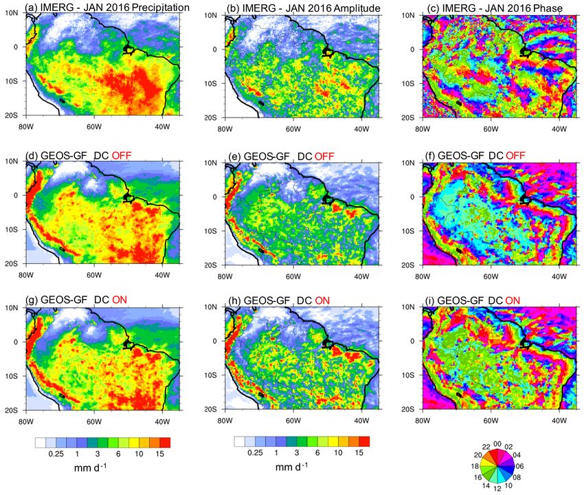
5394                                                             S. R. Freitas et al.: The GF convection parameterization

Environmental Prediction (NCEP) of the National Weather          cohabit a given model grid column. The parameterization is
Service (NWS) in the US, at the Global Modeling and As-          performed over the entire spectrum executing first the shal-
similation Office of NASA Goddard Space Flight Center,           low, next the congestus, and finally the deep mode. In this
and in the Brazilian Center for Weather Forecast and Cli-        manner, the convective tendencies resulting from the devel-
mate Studies (CPTEC/INPE). Scale awareness was evaluated         opment of each mode may be applied as a forcing for the
in a nonhydrostatic global model with smoothly varying grid      next one. In this paper, however, the results shown do not in-
spacing from 50 to 3 km (Fowler et al., 2016) and also in a      clude feedback from the shallower modes. The impacts of a
cascade of global-scale simulations with uniform grid size       successive application will be looked at in a future study.
spanning from 100 km to a few kilometers using the NASA
Goddard Earth Observing System (GEOS) global circulation         2.1.1   Shallow convection
model (GCM) (Freitas et al., 2018, 2020).
   The use of GF in other modeling systems and for other ap-     The source parcels for the shallow convecting plumes are de-
plications required further modifications to represent phys-     fined by mixing the environmental moist static energy (MSE)
ical processes such as momentum transport, cumulus con-          and water vapor mixing ratio over a user-specified depth
gestus clouds, modifications of cloud water detrainment,         layer (currently, the lowest atmospheric layer with 30 hPa
and better representation of the diurnal cycle of convection.    depth). Then, an excess MSE and moisture perturbation as-
These new features are described in this paper.                  sociated with the surface fluxes are added when calculating
   In Sect. 2, we will describe the new implementations and      the forcing and checking for trigger functions, as described
options; Sect. 3 will show some results from both single-        in GF2014. The cloud base is defined by the first model
column models and full 3D simulations, and Sect. 4 will con-     level where the source air parcel lifted from the surface with-
clude and summarize results.                                     out any lateral entrainment is positively buoyant. Above the
                                                                 cloud base, shallow convection growth and cloud properties
                                                                 will strongly depend on the description of the vertical mass
2     New developments and extensions                            flux distribution and resulting entrainment and detrainment
                                                                 rates. Since the BFs are part of all three types of convec-
2.1    The trimodal formulation                                  tion, the method will be described in detail in Sect. 2.2. The
                                                                 shallow convection cloud tops are determined following two
The original unimodal steady-state updraft deep plume has        criteria. One is defined by the first vertical layer at which the
been replaced by a trimodal formulation, which allows up to      buoyancy becomes negative. The second is defined by the
three characteristic convective modes (Johnson et al., 1999):    first thermal inversion layer above the planetary boundary
shallow, congestus, and deep. This approach lies between the     layer (PBL) height. The inversion layer is found following
two extremes of having a single bulk cloud (e.g., Tiedtke,       two conditions:
1989; Grell, 1993, and many others) and a full spectral cloud
                                                                   i. the first derivative (∂T /∂z, where T is the grid-scale air
size approach (e.g., Arakawa and Schubert, 1974; Grell et al.,
                                                                      temperature) must have a local maximum, and
1991; Grell, 1993; Moorthi and Suarez, 1992; Baba, 2019).
To be clear, we are not claiming to represent three plumes,       ii. the absolute value of the second derivative must be zero
but BFs characterizing plumes. For example, the BF for deep           (inflexion point).
convection is a statistical average of deep plumes in the grid
box and may include impacts from several plumes.                 The effective cloud top is defined by the layer that has the
   Each mode of our trimodal formulation is characterized by     lower vertical height. The closures for the determination of
a BF that determines average lateral mixing. For each mode       the mass flux at cloud base, suitable for the shallow moist
we assume a characteristic initial gross lateral entrainment     convection regime, are the following.
rate to represent an approximate size of one of the three           Raymond (1995) establishes the equilibrium for the
modes of convection in the grid box. Section 2.2 provides        boundary layer budget of the moist static energy. In this case,
details on this formulation, including how the entrainment       the flux out at the cloud base of shallow convection counter-
and detrainment rates (lateral mixing) are derived from the      balances the flux in from surface processes. This closure is
BFs. The deep and congestus modes are accompanied by             called boundary layer quasi-equilibrium (BLQE). The BLQE
convective-scale saturated downdrafts sustained by rainfall      closure provides a reasonable diurnal cycle of shallow con-
evaporation. Associated with each mode, a set of closures to     vection over land, as the resulting mass flux at cloud base is
determine the mass flux at the cloud base was introduced to      tightly connected with the surface fluxes. The equation for
adequately account for the diverse regimes of convection in a    the mass flux at cloud base (mb ) from this closure reads
given grid cell. The three modes transport momentum, trac-
                                                                        Rp
ers, water, and moist static energy. For mass and energy, the         − pscb ∂∂th̃ dp
                                                                                    g
spatial discretization of the tendency equation is conserva-     mb =            ,                                          (1)
tive on machine precision. The three modes are allowed to               hc − h̃
                                                                                  cb

Geosci. Model Dev., 14, 5393–5411, 2021                                           https://doi.org/10.5194/gmd-14-5393-2021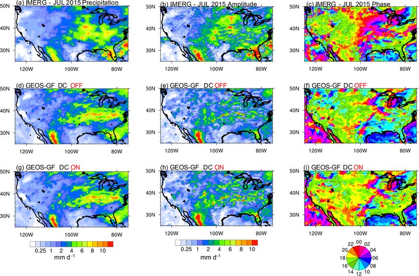
S. R. Freitas et al.: The GF convection parameterization                                                                        5395

where hc and h̃ are the in-cloud and environmental moist            2.2    Representation of normalized vertical mass flux
static energy, respectively, g is gravity, p is pressure, and the          profiles
integral is determined from the surface to the cloud base. h̃
is approximated by the grid-scale moist static energy, and its      The new version applies analytical beta functions to repre-
tendency is given by adding the tendencies from the grid-           sent the average statistical mass flux of the plumes. We as-
scale advection, diffusion in the planetary boundary layer,         sume that the average normalized mass flux profiles for up-
and radiation.                                                      drafts (Zu ) and downdrafts (Zd ) in the grid box may be rep-
   Grant (2001) introduced a closure based on the boundary          resented by a beta function (BF), which is given by
layer convective-scale vertical velocity (w∗ ) and the air den-
sity at the cloud base (ρ). In this closure, mb is simply given     Zu,d (rk ) = crkα − 1(1 − rk )β − 1,                          (4)
by
                                                                    where c is defined below (Eq. 6) as a normalization constant
ρmb = 0.03w .     ∗
                                                             (2)    to ensure that the total integral is 1, rk is the location of the
                                                                    mass flux maximum given by the ratio between the pressure
Rennó and Ingersoll (1996) and Souza (1999) applied the             depth from which the normalized maximum mass flux of the
concept of convection as a natural heat engine to provide a         cloud is in relation to the cloud base related to the total depth
closure for the updraft mass flux at cloud base:                    of the cloud,

         ηFin                                                           p − pbase
mb =          ,                                              (3)    rk =           ,                                              (5)
        TCAPE                                                           pt − pbase
                                                                         0(α + β)
where η is the thermodynamic efficiency, Fin is the buoy-           c=               ,                                            (6)
                                                                       0 (α) + 0(β)
ancy surface flux, and TCAPE is the total convective available
potential energy, which is approximated by the standard con-        α and β determine the skewness of the function, and 0 is
vective available potential energy (CAPE) calculated from           the gamma function. In GF they depend to a large extent
the vertical level of the air parcel source to the cloud top        on where the maximum of the BF is located. For shallow
(Souza, 1999).                                                      and congestus convection, the maximum is located towards
                                                                    the cloud base. For shallow convection, it is assumed to be
2.1.2    Congestus and deep convection                              at or just above the level of free convection. For congestus,
                                                                    we assume this level to be higher at half of the congestus
Congestus and deep convection share several properties and
                                                                    cloud depth. For deep convection, this level is given by the
will be described together in this section. Both allow associ-
                                                                    level where the stability changes sign; the stability is given
ated convective-scale saturated downdrafts (see Grell, 1993,
                                                                    by the difference from in-cloud moist static energy and en-
for further details). As for shallow convection, they are dis-
                                                                    vironmental saturation moist static energy. This is equivalent
tinguished by different characteristic initial gross entrain-
                                                                    to assuming that the strong increase in static stability at those
ment rates (see Sect. 2.2) that represent the deep and con-
                                                                    levels will – statistically – lead to an increase in detrainment
gestus modes. The cloud bases are found following the same
                                                                    and a possible decrease in updraft radius (not necessarily up-
procedure described for the shallow convection. For deep
                                                                    draft vertical velocity). For deep convection, we assume
convection, the cloud top is defined by the vertical layer
where the buoyancy becomes negative. For congestus con-
                                                                                       p − pbase

vection, the thermal inversion layer closest to the 500 hPa         β = 1.3 + 1 −                   .                             (7)
                                                                                         1200
pressure level defines the cloud top for the congestus mode.
   The closure formulations to determine the cloud-base             Then, α is imply given by
mass fluxes for deep convection are described in GD2002.
For congestus, the closures BLQE (Eq. 1) and based on w∗                   rkm (β − 2) + 1
                                                                    α=                     ,                                      (8)
(Eq. 2) described in Sect. 2.1.1 are available, as is the insta-               1 − rkm
bility (measured as the cloud work function) removal using
a prescribed timescale of 1800 s (see Sect. 2.3 for further de-     where rkm is the value of rk at the level of maximum mass
tails).                                                             flux. α and β determine the skewness of the BF. For shallow
                                                                    convection we use β = 2.2 and for congestus convection β =
                                                                    1.3. The downdrafts are assumed to reach maximum mass
                                                                    flux – in a statistical sense – at or below cloud base; therefore,
                                                                            p − p(1)
                                                                    rk =                 ,                                        (9)
                                                                           pstart − p(1)

                                                                    with β = 4pstart here as the downdraft originating level.

https://doi.org/10.5194/gmd-14-5393-2021                                                Geosci. Model Dev., 14, 5393–5411, 2021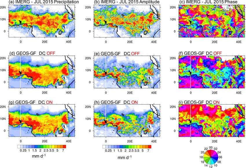
5396                                                                 S. R. Freitas et al.: The GF convection parameterization

   Once the normalized mass flux profiles are defined, the
entrainment and detrainment rates are adjusted accordingly.
First, an initial entrainment rate is given that is meant to char-
acterize the type of convection in the grid box. This is as-
sumed to be the initial rate at the cloud base. In the version of
the parameterization that is used in the Rapid Refresh hourly
update cycle at the National Weather Service of the US (here-
after RAP) and is available to the community using GitHub,
we use

γ (z) = 7 × 10⁻⁵ , 3 × 10⁻⁴ , 1 × 10⁻³                      (10a)

for deep, congestus, and shallow convection, respectively,           Figure 1. The universe of solutions for the normalized updraft mass
                                                                     flux profile (Zu ) for a case in which the cloud base resides at 1.2 km
with
                                                                     of height, the height of maximum Zu is 4.3 km, and the cloud top
                                                                     is at 15.1 km of height. The horizontal axis denotes the range of
δ (z) = 0.1 γ (z) , 0.5 γ (z) , 0.75 γ (z) ,                (10b)
                                                                     variation of the beta parameter. The white contour lines delimit the
                                                                     solution domain where Zu ∈ [0.99, 1.].
where γ , δ represents the entrainment and detrainment rates
(m−1 ). With initial γ , δ, and the PDFs for Zu defined, the
effective lateral mixing (given through entrainment and de-
trainment rates γ ∗ and δ ∗ ), in a statistically averaged sense,
must be related to the vertical mass flux profiles. They are
simply given by
                1 dZu

 ∗              Zu dz    + δ (z) , z ≤ zmax
γ (z) =                                                     (11a)
                γ (z) , z > zmax ,

                δ (z) ,    z ≤ zmax
δ ∗ (z) =          1 dZu                                    (11b)
                − Zu dz + γ (z) , z > zmax ,

where z is the vertical height and zmax is the vertical height
at which the maximum value of Zu is located. A comparison            Figure 2. The universe of solutions for the effective net mass ex-
                                                                     change rate (entrainment – detrainment, km−1 ) for the case shown
to observed mass flux profiles using a single-column model
                                                                     in Fig. 1. The black contour lines demark the transition from mostly
approach is given in Fig. 4 and described later in this section
                                                                     entraining to mostly detraining plumes.
in more detail.
   The use of BFs enables interesting options for introducing
completely mass-conserving stochastic parameter perturba-            The rmax is used to move the level of maximum mass flux up
tions (SPPs) with a possibly significant increase in spread. It      or down, and the β is used to define the shape of the profile.
may of course also be used for training and tuning purposes.         The allowed range of the beta parameter is [1, 5]. For ex-
The operational version of the RAP uses the GF scheme with           ample, Fig. 1 introduces the universe of solutions for Zu of
BFs without tuning and so far without any stochastic appli-          the deep convection updraft for a case in which the heights
cations. However, we are also planning on using some of the          of cloud base, maximum mass flux, and the cloud top are
approaches described next for SPP stochastics in the near fu-        1.2, 4.3, and 15.1 km, respectively. Choosing β closer to 1
ture. In the next section we will describe possible ways to          results in a very gentle shape of the mass flux in the tropo-
apply stochastics and/or use this approach for tuning.               sphere, but with a very sharp increase (decrease) at cloud
                                                                     base (cloud top) with large entrainment (detrainment) mass
2.3    Options for stochastic approaches
                                                                     rates. Increasing β, the profile becomes curved and, above
Following from Sect. 2.2 and Eq. (4), we use the requirement         the level of maximum Zu , the detrainment rates dominate
                                                                     over the entrainment. An appropriate choice of the β param-
dZu,d                                                                eter implies, for example, a more even detrainment of con-
                   = 0 H⇒ f (α, β, rmax ) = 0,               (12)    densate water through the upper troposphere or a sharper,
 drk    rk =rmax
                                                                     narrower detrainment at the very deep cloud-top layer.
where rmax relates to the vertical level at which the mass flux         To give an example, using Eqs. (10) and (11), zmax is
profile reaches its maximum value. In this way, the function         defined as 4.3 km in Fig. 1. Figure 2 introduces the differ-
is unequivocally defined once β and rmax are specified. The          ence between the effective entrainment and detrainment rates
two parameters β and rmax may be stochastically perturbed.           (γ ∗ − δ ∗ ) for the case shown in Fig. 1. Assuming β closer to 1

Geosci. Model Dev., 14, 5393–5411, 2021                                                https://doi.org/10.5194/gmd-14-5393-2021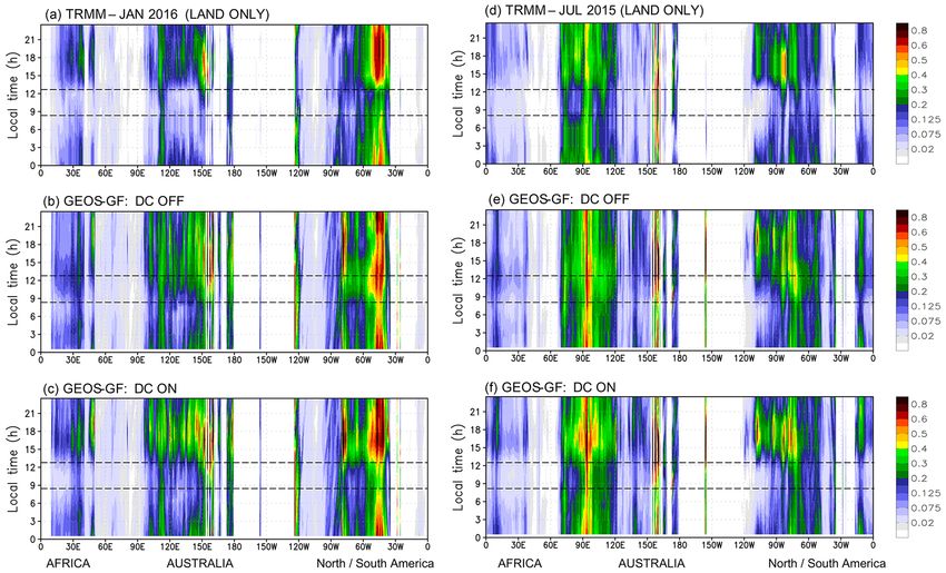
S. R. Freitas et al.: The GF convection parameterization                                                                      5397

                                                                     areas. Moreover, as models configured at cloud-resolving
                                                                     scales can intrinsically capture the diurnal cycle of con-
                                                                     vection, global models with good skill in the diurnal cycle
                                                                     representation should yield a smoother transition from non-
                                                                     resolved to resolved scales. Lastly, it seems plausible that
                                                                     benefits for the data assimilation are also expected with a
                                                                     better diurnal cycle representation.
                                                                        In the effort to improve the diurnal cycle in the GF scheme,
                                                                     we adopted a closure for nonequilibrium convection devel-
                                                                     oped by Bechtold et al. (2014, hereafter B2014), which, as
                                                                     we further demonstrate, notably improves the simulation of
                                                                     the diurnal cycle of convection and precipitation over land.
                                                                     B2014 proposed the following equation for the convective
                                                                     tendency for deep convection, which represents the stabi-
                                                                     lization response in the closure equation for the mass flux
Figure 3. Total (red solid), convective (red dashed), and observed
                                                                     at cloud base:
total precipitation rates (mm per hour) with the GF scheme using
the TWP-ICE soundings.                                               ∂5               5 τBL ∂5
                                                                                 =−     +                        ,             (13)
                                                                     ∂t   conv        τ   τ ∂t              BL

implies a very large effective entrainment and detrainment at        where 5 is called the density-weight buoyancy integral, and
cloud base and top with very small net mass exchange in be-          τ and τBL are appropriate timescales. The tendency of the
tween. Increasing β makes the entrainment and detrainment            second term on the right side of Eq. (13) is the total boundary
layers wider and smoother.                                           layer production given by
   The above-described options for stochastically perturbing
vertical mass flux distributions may also be used in fine tun-                            Zpb
                                                                     ∂5         1               ∂Tv
ing of model performance, in particular for operational fore-                =− ∗                          dp,                 (14)
casting applications. Those parameters allow slight changes          ∂t   BL   T                 ∂t
                                                                                          ps          BL
in the vertical distribution of heating and drying and may be
used to improve biases in temperature and moisture profiles.         where the virtual temperature tendency includes tendencies
As is the case with parameters and assumptions in convective         from grid-scale advection, diffusive transport, and radiation.
parameterizations in general, the values proposed in Sect. 2.2       T ∗ is a scale temperature parameter, and the integral is per-
may, of course, not be universal, and optimal values may             formed from the surface (ps ) to the cloud base (pb ). The
need adjustments for each host model.                                justification for subtracting a fraction of the boundary layer
                                                                     production is that 5 already contains all the boundary layer
2.4   Diurnal cycle closure                                          heating but it is not totally available for deep convection.
                                                                        In GF, we follow B2014 to introduce an additional clo-
Convection parameterizations based on the use of CAPE for            sure using the concept of the cloud work function (CWF)
closure and/or trigger function prove difficult in accurately        available for the deep convection overturning. The CWF is
representing the diurnal march of convection and precipi-            calculated as
tation associated with the diurnal surface heating in an en-
vironment of weak large-scale forcing. In nature, shallow                 Zzt
                                                                                 1 Zu             ∗
and congestus convective plumes start a few hours after sun-         A=                    (hu − h ) gdz ,                     (15)
rise, moistening and cooling the lower and mid-troposphere.                     cp T 1 + γ
                                                                          zb
These physical processes prepare the environment for the
deep penetrative and larger rainfall-producing convection,           where A is the total updraft CWF, zb and zt are the height of
which usually occurs in the mid-afternoon to early evening.          the cloud base and cloud top, respectively, g is the gravity,
Models, in general, simulate a more abrupt transition, with          cp is the specific heat of dry air, Zu is the normalized mass
                                                                                                                            ∗
the rainfall peaking in phase with the surface fluxes, earlier       flux, T is the grid-scale air temperature, and hu and h are the
than observations indicate (Betts and Jakob, 2002).                  updraft and grid-scale saturated moist static energy, respec-
   In addition to a more accurate timing of the precipitation        tively. The parameter γ is given by Grell (1993, Eq. A15).
forecast, a realistic representation of the diurnal cycle in a       Following B2014, the boundary layer production is given by
global model should also improve the forecast of the near-
surface maximum temperature. Additionally, it improves the                         Zzb
                                                                          τBL             ∂Tv
subgrid-scale convective transport of tracers, which should          ABL = ∗                          gdz ,                    (16)
                                                                          T                ∂t
be especially relevant for carbon dioxide over vegetated                          zsurf         BL

https://doi.org/10.5194/gmd-14-5393-2021                                                   Geosci. Model Dev., 14, 5393–5411, 2021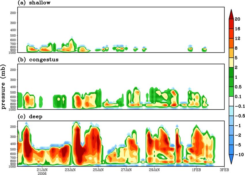
5398                                                                     S. R. Freitas et al.: The GF convection parameterization

Figure 4. (a) On the left is the two-season mean mass flux associated with all cumulus clouds (solid curves), congestus (dotted), deep
(dashed), and overshooting convection (dotted–dashed) using wind-profiler (black) and CPOL-based (red) measurements taken at the profiler
site (From Kumar et al., 2016, © American Meteorological Society; used with permission). (b) On the right are the TWP-ICE mean mass
flux (kg m2 s−1 ) profiles from all cumulus clouds (in black), shallow (in blue), congestus (in green), and deep convection (in red) with GF
SCM simulation.

Figure 5. Convective heating tendencies (K d−1 ) of (a) shallow, (b) congestus, and (c) deep convection with the GF scheme using the
TWP-ICE soundings.

where τBL is the boundary layer timescale given by B2014                   While the impact for the GEOS modeling system was a
(Eq. 15 therein) and the integral is performed from the sur-            substantial improvement, this may depend on other physical
face (zsurf ) to the cloud base. From Eqs. (15) and (16), the           parameterizations and how tendencies are applied in a GCM.
available CWF (Aavail ) is given by                                     For this reason, in GF this closure is optional. It can be com-
                                                                        bined with any of the other closures previously available in
Aavail = A − ABL ,                                            (17)      the scheme for deep convection.
and the rate of instability removal is given by Aavail /τ , where
τ is a prescribed timescale that is currently 1 and 0.5 h for
deep and congestus modes, respectively.

Geosci. Model Dev., 14, 5393–5411, 2021                                                   https://doi.org/10.5194/gmd-14-5393-2021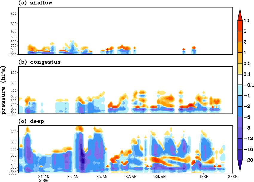
S. R. Freitas et al.: The GF convection parameterization                                                                          5399

Figure 6. Convective drying tendencies (g kg−1 d−1 ) of (a) shallow, (b) congestus, and (c) deep convection with the GF scheme using the
TWP-ICE soundings.

2.5   Inclusion of the ice-phase process                              the entrained environmental air. Overall, the associated ad-
                                                                      ditional heating has a small impact on the total convective
The thermodynamical equation employed in the GF scheme                heating tendency.
uses the moist static energy (h) as a conserved quantity for             The partition between liquid- and ice-phase contents
non-entraining air parcels with adiabatic displacements:              is represented by a smoothed Heaviside function that in-
                                                                      creases from 0 to 1 in the finite temperature range [235.16,
dh = 0,                                                     (18)      273.16] K, which is given by fract_liq = min(1, (max(0, (T −
where h has the usual definition,                                     235.16))/(273.16 − 235.16))2 ).
                                                                         The melting of precipitation falling across the freezing
h = cp T + gz + Lv qv ,                                     (19)      level is represented by adding an extra term to the grid-scale
                                                                      moist static energy tendency:
and cp is the isobaric heat capacity of dry air, T is the tem-              !
perature, g is the gravity, z is the height, Lv the latent heat         ∂h             g Lf M
                                                                                  =−          ,                                 (22)
of vaporization, and qv the water vapor mixing ratio. How-               ∂t              1p
                                                                              melt
ever, h is not conserved if glaciation transformation occurs,
and this process was not explicitly included in GF until now.         where M is the mass mixing ratio of the frozen precipitation
Incorporating the transformation of liquid water to ice parti-        that will melt in a given model vertical layer of the pressure
cles, Eq. (18) now reads                                              depth 1p.

dh = Lf qi ,                                                (20)
                                                                      3     Applications
where Lf is the latent heat of freezing, and qi is the ice mixing
ratio. With the extended Eq. (20), the general equation for the       In this section, applications associated with the features de-
in-cloud moist static energy including the entraining process         scribed in the previous section are discussed.
solved in this version of GF is
                                                                      3.1    The trimodal characteristics revealed by
dh = Lf qi + (dh)entr ,                                     (21)             single-column simulations

where (dh)entr represents the modification of the in-cloud            The GF convection scheme was implemented into the Com-
moist static energy associated with the internal mixing with          mon Community Physics Package (CCPP) Single Column

https://doi.org/10.5194/gmd-14-5393-2021                                                   Geosci. Model Dev., 14, 5393–5411, 2021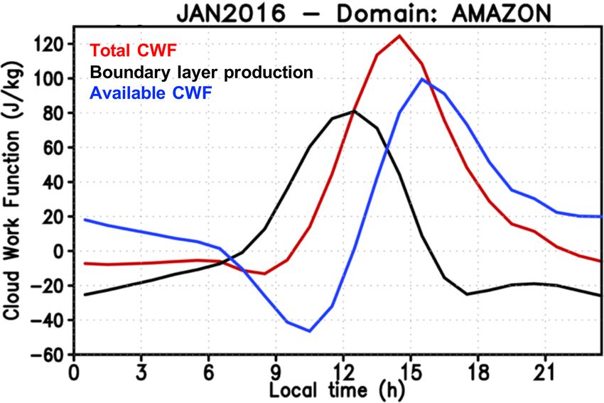
5400                                                               S. R. Freitas et al.: The GF convection parameterization

Model (SCM; Firl et al. 2018), and SCM simulations were
executed using data (Xie et al., 2010) from the Tropical
Warm Pool International Cloud Experiment (TWP-ICE; May
et al., 2008) to demonstrate the trimodal characteristics and
the value of using BFs. TWP-ICE is a comprehensive field
campaign that took place in January and February 2006 over
Darwin, Australia.
   Strong precipitation events are observed during the active
monsoon period with a major mesoscale convective system
(MCS) on 23 January 2006, followed by a suppressed mon-
soon with relatively weak rainfall (Fig. 3). The periods 19–
25 January and 26 January–2 February 2006 are defined as
active monsoon and suppressed monsoon periods for the sub-
sequent quantitative analysis. As shown in Fig. 3, GF cap-
tures all the peak precipitation events during the active mon-
soon period. The heavy precipitation in the active monsoon
period appears underestimated, while the light precipitation
events in the suppressed monsoon period may be overesti-
mated. However, exact agreement cannot be expected. Pre-
cipitation data for this data set were derived from radar data;
derivation of large-scale forcing data is also not trivial. Some
of this is also obvious in the calculation and discussion of
the Q1 and Q2 profiles (later in this section). The convective
precipitation contributes about 78 % of the total precipitation
during the active monsoon period and contributes as much
as 94 % of total precipitation during the suppressed monsoon
period.
   To test the approximation of the normalized mass flux with
our generalized normalized mass flux approach, we compare          Figure 7. The diabatic heating source (Q1, K d−1 ) profiles from
the simulated mass flux profiles with observations, as ana-        (a) sounding analysis, (b) SCM simulation, and diabatic drying sink
lyzed by Kumar et al. (2016). Of particular importance for         (Q2, K d−1 ) from (c) sounding analysis and (d) SCM simulation.
us is whether the predicted mass flux for deep convection is       The active monsoon period is in red, and the suppressed period is in
able to characterize deep convective clouds in the area, since     green.
this will determine maximum entrainment and detrainment
in the GF parameterization. For completeness we also com-
pare congestus and shallow clouds. The mean mass flux dur-         Temperature tendencies are derived using
ing the whole TWP-ICE simulation period from all cumulus           ∂T    1                    Lv
clouds (deep, congestus, and shallow) is shown in Fig. 4b.            =    % [h (z)] mb(CU) −    % q (z) mb(CU) .                 (23)
                                                                   ∂t   cp                    cp
The congestus mass flux (green), which is weaker than the
mass flux for deep convection, has its maximum at around           Here, % is the change in moist static energy (h) or water vapor
7 km of height. The maximum mass flux from deep convec-            (q) per unit mass, and mb(CU) is the cloud-base mass flux for
tion (red) and all convective types (black) is around 6 km and     deep, congestus, or shallow convection.
a bit under 6 km, respectively. Kumar et al. (2016) estimated         More low-level heating due to shallow convection occurs
the convective mass flux for two wet seasons (October 2005–        during the active monsoon stage. The congestus (Fig. 5b) and
April 2006 and October 2006–April 2007) from radar obser-          deep (Fig. 5c) convection cools the boundary layer mainly
vations over Darwin, Australia. Although the TWP-ICE sim-          through downdrafts and evaporation of rainfall, and it also
ulation period (19 January–2 February 2006) is much shorter,       cools the troposphere through the evaporation of detrained
the shape of the mass flux profiles in Fig. 4b is quite similar    cloud condensates at cloud tops. On 23 January 2006, the
to their observations, shown in Fig. 4a, which is from Fig. 13     strong heating from the lower troposphere to 500 and 200 hPa
of Kumar et al. (2016, © American Meteorological Society;          for congestus and deep convection, respectively, corresponds
used with permission).                                             to the heavy precipitation in Fig. 3. Figure 6 shows the con-
   Figure 5 shows the convective heating rate of shallow           vective drying tendencies of shallow (Fig. 6a), congestus
(Fig. 5a), congestus (Fig. 5b), and deep convection (Fig. 5c).     (Fig. 6b), and deep convection (Fig. 6c). The entraining of
In the case of the shallow convection (Fig. 5a) the environ-       low-level environmental moist air into the convection plumes
ment is warmed in the lower levels and cooled at cloud tops.       and raining out results in drying of the lower atmosphere,

Geosci. Model Dev., 14, 5393–5411, 2021                                              https://doi.org/10.5194/gmd-14-5393-2021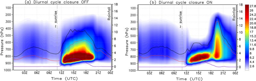
S. R. Freitas et al.: The GF convection parameterization                                                                                5401

Figure 8. The diurnal cycle of the three convective modes as represented by the GF convection parameterization in a single-column model
experiment with the GEOS-5 modeling system. The black contours represent the vertical diffusivity coefficient for heat (m2 s−1 ). The color
contours show the updraft mass flux expressed in 10−3 kg m−2 s−1 .

Figure 9. Color shading is the time average of the diurnal cycle of the total vertical mass flux of the three convective modes: shallow,
congestus, and deep (10−3 kg m2 s−1 ). The rainfall is depicted by graphic lines: black, red, and purple represent the total precipitation and
the convective part from deep and congestus plumes, respectively. The scale for rainfall appears on the right vertical axis (mm d−1 ). Panel
(a) represents the results without the diurnal cycle closure, and panel (b) is with.

while the detrained cloud water–ice at the cloud top leads               3.2    Evaluation of the diurnal cycle closure
to some cooling. The strongest drying for deep convection
on 23 January 2006 (Fig. 6c) from the lower troposphere to
                                                                         Santos e Silva et al. (2009, 2012) discussed the diurnal cy-
200 hPa also corresponds to the heavy precipitation in Fig. 4.
                                                                         cle of precipitation over the Amazon Basin in detail using
   The heating and drying features of the single-column
                                                                         the TRMM rainfall product (Huffman et al., 2007), observa-
model (SCM) simulation with the GF convection scheme are
                                                                         tional data from an S-band polarimetric radar (S-POL), and
further validated by the diabatic heating source (Q1) and dry-
                                                                         rain gauges obtained in a field experiment during the wet sea-
ing sink (Q2), which were defined by Yanai et al. (1973),
                                                                         son of 1999. Their analysis indicated that peak in rainfall is
from sounding analysis. The averaged profiles of Q1 and Q2
                                                                         usually late in the afternoon (between 17:00 and 21:00 UTC),
derived from constrained variational objective analysis ob-
                                                                         despite existent variations associated with wind regimes. In
servation (Xie et al., 2010) are shown in Fig. 7a and c, while
                                                                         addition, over the Amazon, a secondary period of convection
the SCM-simulated Q1 and Q2 are given in Fig. 7b and d.
                                                                         activity is observed during the night as reported by Yang et
The shape of Q1 and Q2 in active or suppressed periods from
                                                                         al. (2008) and Santos e Silva et al. (2012). In general, this is
the simulation agrees with the observations very well, but
                                                                         associated with squall line propagation in the Amazon Basin
with a stronger magnitude. The maximum Q1 and Q2 be-
                                                                         (Cohen et al., 1995; Alcântara et al., 2011). This bimodal
tween 350 and 550 hPa in the active monsoon period corre-
                                                                         pattern of convective activity can be identified with observa-
sponds to the heavy precipitation in Fig. 3. The Q1 and Q2
                                                                         tional analysis of vertical profiles of moistening and heating
from observations and simulations were mainly distributed at
                                                                         (Schumacher et al., 2007).
low levels in the suppressed period, consistent with the study
                                                                            Here we evaluate the GF scheme with the B2014 closure
from Xie et al. (2010).
                                                                         by applying it in the NASA GEOS GCM configured as a
                                                                         single-column model (SCM). The GEOS SCM with GF was
                                                                         run from 24 January to 25 February 1999 using the initial
                                                                         conditions and advective forcing from the TRMM_LBA field

https://doi.org/10.5194/gmd-14-5393-2021                                                     Geosci. Model Dev., 14, 5393–5411, 2021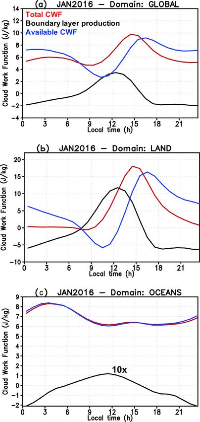
5402                                                                       S. R. Freitas et al.: The GF convection parameterization

Figure 10. Time average of the diurnal cycle of the grid-scale vertical moistening (a, c) and heating (b, d) tendencies associated with the
three convective modes (shaded colors) and precipitation (contour: red dashed, green solid, and purple dashed represent the total precipitation
and the convective precipitation from deep and congestus plumes, respectively). The upper (bottom) panels show results without (with) the
diurnal cycle closure.

                                                                          the PBL top and cloud tops below ∼ 700 and 550 hPa, re-
                                                                          spectively. Those two modes precede the deep convection
                                                                          (Fig. 8c) development during the late afternoon (local time
                                                                          is UTC−4 h) with cloud tops reaching 200 hPa.
                                                                             Figure 9 shows the mean diurnal cycle of the net vertical
                                                                          mass flux (the sum of shallow, congestus, and deep modes)
                                                                          as well as the total and convective precipitation. The chosen
                                                                          closures for the mass flux at cloud base were the BLQE for
                                                                          shallow and the adaptation of B2014 for congestus and deep
                                                                          modes, as described at the end of Sect. 2.3. For congestus,
                                                                          we only retained the first term of Eq. (17); for deep, the sim-
                                                                          ulations were performed without and with the second term of
                                                                          Eq. (17). This allowed us to evaluate its role in defining the
                                                                          phase of the diurnal march of the precipitation.
Figure 11. The monthly mean (January 2016) diurnal variation                 Figure 9a shows the model results without applying the
of the total cloud work function (red), boundary layer production
                                                                          diurnal cycle closure (i.e., retaining only the first term of
(black), and available cloud work function (blue). The curves also
represent the areal average over the Amazon region.
                                                                          Eq. 17) for deep convection. In this case, the three convec-
                                                                          tive modes coexist, triggered just a few hours after sunrise
                                                                          (∼ 11:00 UTC), with the deep convection occurring too early
                                                                          and producing maximum precipitation at about 15:00 UTC
campaign data. The simulation started on 00:00 Z 24 Jan-
                                                                          (∼ 11:00 local time). Conversely, we observed a clear sepa-
uary 1999 with 1-month time integration. Model results were
                                                                          ration between the convective modes when applying the full
averaged in time to express the mean diurnal cycle. An ini-
                                                                          equation of the diurnal cycle closure (Fig. 9b), reducing the
tial glance at the three convection modes in the GF scheme
                                                                          amount of potential instability available for the deep convec-
is given by Fig. 8, where the time-averaged mass fluxes
                                                                          tion. In this case, there is a delay of the precipitation from the
(10−3 kg m−2 s−1 ) of each mode are introduced. The con-
                                                                          deep penetrative convection with the maximum rate taking
tour lines in black represent the vertical diffusivity coeffi-
                                                                          place between 18:00 and 21:00 UTC, more consistent with
cient for heat (m2 s−1 ), describing the diurnal development
                                                                          observations of the diurnal cycle over the Amazon region.
of the planetary boundary layer (PBL) over the Amazon for-
                                                                             Figure 10 introduces the grid-scale vertical moistening
est. The PBL development seems to be well represented with
                                                                          and heating tendencies associated with the three convective
a fast evolution in the first hours after sunrise and stabiliz-
                                                                          modes for the simulations without and with the diurnal cy-
ing around noon with a realistic vertical depth between 1
                                                                          cle closure. The net effect (moistening minus drying) of the
and 1.5 km. Both shallow (Fig. 8a) and congestus (Fig. 8b)
                                                                          three convective modes, not including the diurnal cycle clo-
modes start a few hours after sunrise with cloud base around

Geosci. Model Dev., 14, 5393–5411, 2021                                                     https://doi.org/10.5194/gmd-14-5393-2021
S. R. Freitas et al.: The GF convection parameterization 5403
deep cumulus. Associated with the delay of precipitation, the
peak downdraft occurrence is correspondingly displaced. On
the right, Fig. 10c and d introduce the results for the heating
tendencies. A similar discussion applies to these tendencies,
with the peak of the atmospheric heating delayed by a few
hours, when the diurnal cycle closure is applied (Fig. 10d).
Note that the warming from the congestus plumes somewhat
offsets the low-troposphere cooling associated with the shal-
low plumes.
3.3 Global-scale three-dimensional modeling
A global-scale evaluation of the diurnal cycle closure is
shown in this section applying GF within the NASA GEOS
GCM (Molod et al., 2015). The GEOS GCM was config-
ured with c360 spatial resolution (∼ 25 km) and was run in
free forecast mode for all of January 2016. Each forecast day
covered a 120 h time integration, with output available every
hour. Atmospheric initial conditions were provided by the
Modern-Era Retrospective Analysis for Research and Appli-
cations Version 2 (MERRA-2; Gelaro et al., 2017). The sim-
ulations applied the FV3 nonhydrostatic dynamical core on
a cubed-sphere grid (Putman and Lin, 2007). Resolved grid-
scale cloud microphysics apply a single-moment formulation
for rain, liquid, and ice condensates (Bacmeister et al., 2006).
The longwave radiative processes are represented following
Chou and Suarez (1994), and the shortwave radiative pro-
cesses are from Chou and Suarez (1999). The turbulence pa-
rameterization is a nonlocal scheme primarily based on Lock
et al. (2000), acting together with the local first-order scheme
of Louis and Geleyn (1982). The sea surface temperature is
prescribed following Reynolds et al. (2002).
We first demonstrate the impact of the boundary layer pro-
duction on the cloud work function (CWF) available for the
deep convection overturning. Figure 11 shows the monthly
mean of the diurnal variation of the three quantities given by
Figure 12. The monthly mean (January 2016) diurnal variation of Eqs. (10), (11), and (12). The figure represents the monthly
the total cloud work function (red color), boundary layer production mean (January 2016) diurnal variation of the total cloud work
(black), and available cloud work function (blue). The curves also function, boundary layer production, and available cloud
represent the areal average over (a) the entire globe, (b) the land re- work function, all area-averaged over the Amazon Basin.
gions, and (c) the oceans. In panel (c) the boundary layer production
The total CWF tightly follows the surface fluxes as the
is multiplied by 10 for clarity.
air parcels that form the convective updrafts originate close
to the surface in the PBL. The boundary layer production
presents similar behavior, peaking at noon and developing
sure for the deep mode, appears in the Fig. 10a. As the three negative values during the nights. The combination of the
modes coexist most of the time and as the drying associated two terms following Eq. (17) defines the available CWF for
with the deep precipitating plumes dominates, water vapor convection overturning. A negative range of the available
is drained from the troposphere, with a shallow lower-level CWF, associated with the negative buoyancy contribution be-
layer of moistening associated with the precipitation evapo- low the level of free convection, in the early mornings to ap-
ration driven by downdrafts. However, by including the full proximately noon prevents the model from developing con-
formulation of the diurnal cycle closure (Fig. 10b), a much vective precipitation in that period and shifts the maximum
smoother transition is simulated with a late morning and CWF to late afternoon, which is much closer to the observed
early afternoon low to mid-tropospheric moistening by shal- diurnal cycle of precipitation over the Amazon region.
low and congestus convection, followed by a late afternoon A global perspective of these three quantities is shown in
and early evening tropospheric drying by the rainfall from the Fig. 12. As before, the curves represent the monthly mean
https://doi.org/10.5194/gmd-14-5393-2021 Geosci. Model Dev., 14, 5393–5411, 20215404 S. R. Freitas et al.: The GF convection parameterization
Figure 13. Global Hovmöller diagram (average over latitudes 40◦ S to 40◦ N) of the diurnal cycle of precipitation (mm h−1 ) from remote-
sensing-derived observations (TRMM, a, d) and the NASA GEOS GCM applying the GF scheme without the diurnal cycle closure (b, e, DC
OFF) and with (c, f, DC ON). The results account for precipitation only over land regions and are monthly means for January 2016 (a, b, c)
and July 2015 (d, e, f), respectively.
(January 2016) diurnal variation of the total cloud work func- and 40◦ N taking into account only the land regions. The ver-
tion, boundary layer production, and available cloud work tical axis represents the local time.
function. Here the averaged area corresponds to the global The TRMM estimation evidences two peaks of precipi-
domain (Fig. 12a), only the land regions (Fig. 12b), and only tation rate: a nocturnal peak around 03:00 LST over oceans
the oceans (Fig. 12c). Over oceans, the boundary layer pro- (not shown) and another one in late afternoon (15:00 to
duction is small in comparison with the total CWF; over land 18:00 LST) over land. A significant gap of rainfall in the
(Fig. 12b), it is comparable in magnitude with the total CWF, mornings is also seen in both months. We found somewhat
pushing the available CWF to peak closer to the late after- of an overestimation of the precipitation in comparison with
noons and early evenings. On global average (Fig. 12a), the the estimates produced by the TRMM retrieval technique
boundary layer production still plays a substantial role, with (Fig. 13a and d). However, the simulations that apply the di-
a clear effect on the timing of the maximum available CWF. urnal cycle closure (Fig. 13c and f) are superior regarding the
A perspective of the precipitation simulation with the phase in comparison with the simulations that apply the total
GEOS-5 GCM with the GF scheme and the impact of the di- CWF (Fig. 13b and e) for the closure. As shown in Fig. 13c
urnal cycle closure is provided by Fig. 13. Here, the January and f, the diurnal cycle closure adapted from B2014 used in
2016 (left column) and July 2015 (right column) averages of these simulations shows a much better representation of the
the diurnal cycle of precipitation are depicted. Figure 13a and morning to early afternoon gap of the precipitation, which
d show the rainfall estimation by the TRMM Multi-satellite peaks much closer to the time of TRMM retrieval. In par-
Precipitation Analysis (TMPA version 3B42; Huffman et al., ticular, model improvements are noticeable over the Amazon
2007). Also, the precipitation simulated by the GEOS GF, in- region (denoted by “South America”). Similar improvements
cluding the diurnal cycle closure (at middle, Fig. 13c and e) are also evident over Africa and Australia.
or not (lower panels, Fig. 13d and f), is depicted. The precip- For a more detailed analysis of the diurnal cycle of the pre-
itation fields were averaged over the latitudes between 40◦ S cipitation we use higher-spatial- and temporal-resolution re-
trievals from the Global Precipitation Measurement (GPM)
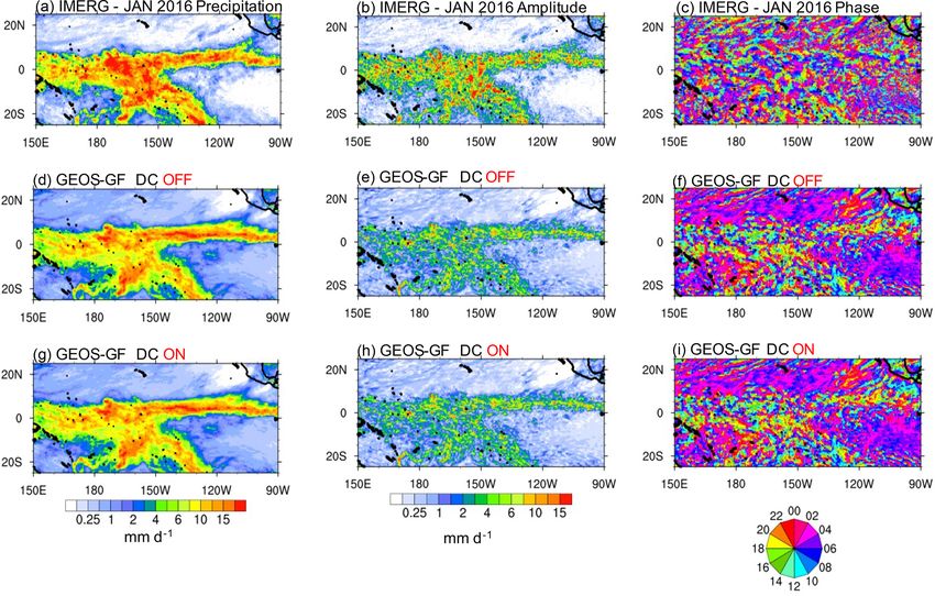
Geosci. Model Dev., 14, 5393–5411, 2021 https://doi.org/10.5194/gmd-14-5393-2021S. R. Freitas et al.: The GF convection parameterization 5405 Figure 14. The January 2016 monthly mean precipitation, amplitude, and phase of the diurnal harmonic over the Amazon Basin. The top panels (a–c) show the quantities of the GPM IMERG retrieval. In the middle (d–f) and lower rows (g–i), panels show model simulations with the diurnal cycle closure turned off and on, respectively. with the Integrated Multi-satellitE Retrievals for GPM the maximum accumulated precipitation occurring south of (IMERG, version 6; Huffman et al., 2019). The IMERG has the Equator following the annual southward shift of the In- 0.1◦ spatial and 1/2 h temporal resolutions. Also, we adopt tertropical Convergence Zone (ITCZ). The domain average the technique of calculating the diurnal harmonics using a precipitation estimated by IMERG was 5.62 mm d−1 . The Fourier transform and focus on the phase and amplitude of correspondent field as simulated by GEOS-5 is shown in the first harmonic. The GPM IMERG retrievals were first in- Fig. 14d and g without (DC OFF) and with (DC ON) the terpolated to the GEOS-5 grid spatial resolution (∼ 25 km) adaptation of the B2014 diurnal cycle closure, respectively. and temporal accumulation (1 h). Figure 14 shows the mean Both simulations show a very similar pattern, and they are precipitation and the mean amplitude and phase of the first also reasonably comparable with the IMERG in the inner part harmonic over the Amazon Basin. The diurnal phase was of the continent. However, the simulations suffer from spu- shifted to the local solar time (LST), and 12:00 LST is associ- rious precipitation along the Andes mountains triggered by ated with the time of maximum insolation in a cloud-free sky numerical noise associated with the steep terrain and the use condition. The IMERG mean precipitation (Fig. 14a) shows of a sigma-type vertical coordinate. The simulated domain the typical summer pattern over the Amazon Basin, with average precipitation was 6.69 (6.59) mm d−1 for the case https://doi.org/10.5194/gmd-14-5393-2021 Geosci. Model Dev., 14, 5393–5411, 2021
5406                                                                    S. R. Freitas et al.: The GF convection parameterization

Figure 15. The January 2016 monthly mean precipitation, amplitude, and phase of the diurnal harmonic over the tropical Pacific Ocean. The
top panels (a–c) show the quantities of the GPM IMERG retrieval. In the middle (d–f) and lower rows (g–i), panels show model simulations
with the diurnal cycle closure turned off and on, respectively.

DC OFF (ON), which is roughly 18 % larger than IMERG. It               (Fig. 14f) simulates a maximum amplitude too early, between
seems plausible that the precipitation excess is mostly associ-        10:00 and 14:00 LT, whereas the case with the diurnal cycle
ated with the spurious generation along the steep terrain. The         ON (Fig. 14i) is closer to the timing of the IMERG (Fig. 14c),
central column of Fig. 14 shows the January 2016 mean am-              with the peaks occurring between 14:00 and 18:00 LT.
plitude of IMERG (panel b) and model simulations (panels e                Correspondent analysis over the tropical Pacific Ocean
and h). The domain average amplitude corresponds to 61, 51,            for January 2016 is included in Fig. 15; the domain aver-
and 62 % of the precipitation of IMERG, model DC OFF, and              age precipitation estimated by IMERG was 4.53 mm d−1 ,
DC ON, respectively. The right column of Fig. 14 shows the             whereas GEOS-5 with DC OFF and DC ON simulated
diurnal phase of the three data sets. Following Kousky (1980)          ∼ 4.21 mm d−1 in both configurations. For the amplitudes,
the maximum precipitation, which forms just inland along               the amounts were 2.16, 1.47, and 1.45 mm d−1 , respectively.
the coast in the late afternoon, is associated with the develop-       The left column of Fig. 15 shows that the spatial distribu-
ment of the sea breeze front. With the sea breeze penetrating          tion of the precipitation simulated by GEOS-5 (panels d and
further inland, another maximum occurs during the nighttime            g) remarkably resembles the IMERG retrieval (panel a), al-
due to the convergence formed with the onshore flow. Both              though the domain average precipitation amounts are under-
features are present in the simulations (Fig. 14f and i), but          estimated by about ∼ 10 %. The former discussion also ap-
the case DC ON better simulates the timing, being closer to            plies to the amplitudes, as shown in the central column of
the IMERG. As for the Amazon Basin interior, the IMERG                 Fig. 15. For the phase, most of the precipitation peaks oc-
shows a nighttime maximum associated with the squall lines             cur through the nighttime (panel c), and the simulations with
that form along the northern coast of Brazil and propagate             GEOS-5 have a similar pattern. The fact that both simula-
long distances across the basin (Alcântara et al., 2011). Both         tions are nearly the same in terms of the precipitation amount
simulations were unable to capture the propagation of these            and its diurnal cycle over the ocean is explained by Fig. 12c.
convective lines. However, it is clear that the case DC OFF

Geosci. Model Dev., 14, 5393–5411, 2021                                                 https://doi.org/10.5194/gmd-14-5393-2021
S. R. Freitas et al.: The GF convection parameterization                                                                            5407

Figure 16. The July 2015 monthly mean precipitation, amplitude, and phase of the diurnal harmonic over a portion of equatorial Africa. The
top panels (a–c) show the quantities of the GPM IMERG retrieval. In the middle (d–f) and lower rows (g–i), panels show model simulations
with the diurnal cycle closure turned off and on, respectively.

   The diurnal cycle of precipitation of the north equatorial          gions, the model’s monthly mean spatial distribution of the
portion of Africa for July 2015 is discussed based on the              precipitation looks realistic, although it underestimates the
results shown in Fig. 16. The domain average precipitation             amount in the southeast and overestimates the rainfall over
(amplitude) is 2.51 (2.12), 2.79 (1.45), and 2.8 (1.8) mm d−1          the eastern part of Gulf of California. According to IMERG,
for panels a (b), d (e), and g (h), respectively. Note that the        the peaks of precipitation occur in the late afternoon over
simulated mean precipitation amounts are about 11 % larger             the southeast and central-western part of the region and in
than the IMERG estimation. For the diurnal phase (Fig. 16c),           the nighttime over the central-eastern part of the domain
the IMERG retrieval shows a mix of late afternoon (16:00–              (Fig. 17c). Over the central part of the US, both simulations
20:00 LT) and nighttime (00:00–04:00 LT) maximum ampli-                did not capture the nighttime precipitation well. However, the
tudes. As before, the simulations show contrasting results for         simulation DC ON (Fig. 17i) seems to be closer to IMERG
the timing of precipitation. Without the diurnal cycle clo-            over the central-western portion.
sure, the precipitation peaks occur too early (mostly 10:00–
14:00 LT, Fig. 16f), whereas with that closure, those peaks
take place mainly after 14:00–16:00 LT (Fig. 16i).                     4    Conclusions
   Figure 17 displays the results for July 2015 over the con-
                                                                       We describe a set of new features recently implemented in
tiguous United States and part of the neighboring countries.
                                                                       the GF convection parameterization. The main new aspects
The domain average precipitation (amplitude) is 2.60 (2.37),
                                                                       are as follows.
2.52 (1.59), and 2.42 (1.8) mm d−1 for panels a (b), d (e),
and g (h), respectively. Model simulations underestimate the               – The unimodal approach has been replaced by a trimodal
mean precipitation by about 5 %–10 %. As in the other re-                    formulation representing the three modes: shallow, con-
                                                                             gestus, and deep convection. Each mode has a distinct

https://doi.org/10.5194/gmd-14-5393-2021                                                   Geosci. Model Dev., 14, 5393–5411, 2021
5408 S. R. Freitas et al.: The GF convection parameterization
Figure 17. The July 2015 monthly mean precipitation, amplitude, and phase of the diurnal harmonic over the contiguous United States and
part of the neighboring countries. The top panels (a–c) show the quantities of the GPM IMERG retrieval. In the middle (d–f) and lower rows
(g–i), panels show model simulations with the diurnal cycle closure turned off and on, respectively.
initial gross entrainment and a set of closure formula- model skill by removing water vapor and temperature
tions for the mass flux at the cloud base. biases.
– An optional closure for nonequilibrium convection up-
– The normalized mass flux profiles are now prescribed dated from Bechtold et al. (2014) is available. This clo-
following a continuous and smooth beta function. From sure has significantly improved the GF scheme’s ability
the cloud base, cloud top, and a free parameter that in the NASA GEOS GCM to represent the diurnal cycle
shapes the BF, the normalized mass flux profile and the of convection over land, also with potential beneficial
entrainment and detrainment rates are determined. To- impacts on data assimilation and tracer transport.
gether with the mass flux at the cloud base defined by
the selected closure, these parameters also determine, The new features of the GF scheme, as described in this
e.g., the vertical drying and heating tendencies associ- paper, further extend the capabilities of this convection pa-
ated with the subgrid-scale convection. Using a BF to rameterization to be applied to a wide range of spatial scales
and environmental problems.
describe the statistical average of a characteristic con-
vection type means that the BF may in fact represent
several plumes in the grid box. Additionally, this ap-
Code availability. The GF convection scheme within
proach may be used to implement stochasticism with
the Global Model Test Bed (GMTB) Single Column
temporal and spatial correlations as well as memory de- Model is available from the GMD-paper branch at
pendence that lead to significant changes in the verti- https://github.com/GF-GMD/ccpp-physics (last access: 26 Au-
cal distribution of heating and drying without disturbing gust 2021), https://doi.org/10.5281/zenodo.5278281 (Li et al.,
mass conservation. Future work will address this possi- 2021). Public access to the NASA GEOS GCM source code
bility. Finally, the use of the BFs may help fine-tune the is available at https://github.com/GEOS-ESM/GEOSgcm (last
Geosci. Model Dev., 14, 5393–5411, 2021 https://doi.org/10.5194/gmd-14-5393-2021S. R. Freitas et al.: The GF convection parameterization 5409
access: 25 August 2021) on tag Jason-3.0. The authors are available Bacmeister, J. T., Suarez, M. J., and Robertson, F. R.: Rain reevapo-
for recommendations on applying the several options present in the ration, boundary layer-convection interactions, and Pacific rain-
GF scheme, as well as for instructions for its implementation in fall patterns in a AGCM, J. Atmos. Sci., 63, 3383–3403, 2006.
other modeling systems. Bechtold, P., Semane, N., Lopez, P., Chaboureau, J., Beljaars, A.,
and Bormann, N.: Representing Equilibrium and Nonequilibrium
Convection in Large-Scale Models, J. Atmos. Sci., 71, 734–753,
Data availability. The data can be obtained from the https://doi.org/10.1175/JAS-D-13-0163.1, 2014.
ARM website at https://www.arm.gov/research/campaigns/ Benjamin, S. G., Weygandt, S. S., Brown, J. M., Hu, M., Alexander,
twp2006twp-ice (last access: 27 August 2021) and C. R., Smirnova, T. G., Olson, J. B., James, E. P., Dowell, D. C.,
https://doi.org/10.5281/zenodo.5292370 (Li, 2021). Grell, G. A., Lin, H., Peckham, S. E., Smith, T. L., Moninger, W.
R., Kenyon, J. S., and Manikin, G. S.: A North American hourly
assimilation and model forecast cycle: The Rapid Refresh, Mon.
Author contributions. SRF and GAG developed the model code Weather Rev., 144, 1669–1694, https://doi.org/10.1175/MWR-
and performed the simulations. HL conducted the simulations and D-15-0242.1, 2016.
produced the results shown in Sect. 3.1. All authors prepared the Betts, A. K. and Jakob, C.: Study of diurnal cycle of convective pre-
paper. cipitation over Amazonia using a single column model, J. Geo-
phys. Res., 107, 4732, https://doi.org/10.1029/2002JD002264,
2002.
Chou, M.-D. and Suarez, M. J.: An efficient thermal infrared ra-
Competing interests. The authors declare that they have no conflict
diation parameterization for use in general circulation models,
of interest.
NASA Tech. Memorandum 104606 – Vol. 3, NASA, Goddard
Space Flight Center, Greenbelt, MD, 1994.
Chou, M.-D. and Suarez, M. J.: A Solar Radiation Parameterization
Disclaimer. Publisher’s note: Copernicus Publications remains for Atmospheric Studies, NASA Tech. Memorandum 104606 –
neutral with regard to jurisdictional claims in published maps and Vol. 15, NASA, Goddard Space Flight Center, Greenbelt, MD,
institutional affiliations. 1999.
Cohen, J. C. P., Silva Dias, M. A. F., and Nobre, C. A.: Environ-
mental conditions associated with Amazonian squall lines: a case
Acknowledgements. The first author acknowledges the support of study, Mon. Weather Rev., 123, 3163–3174, 1995.
NASA/GFSC – USRA/GESTAR grant no. NNG11HP16A. This Firl, G., Carson, L., Bernardet, L., and Heinzeller, D.: Global
work was also supported by the NASA Modeling, Analysis, and Model Test Bed Single Column Model v2.1 User and Technical
Prediction (MAP) program. Computing was provided by the NASA Guide, 26 pp., available at: https://dtcenter.org/sites/default/files/
Center for Climate Simulation (NCCS). community-code/scm-ccpp-guide-v2-1.pdf, last access: 26 Au-
gust 2021.
Fowler, L. D., Skamarock, W. C., Grell, G. A., Freitas, S.
Financial support. This research has been supported by R., and Duda, M. G.: Analyzing the Grell-Freitas con-
NASA/GFSC – USRA/GESTAR (grant no. NNG11HP16A). vection scheme from hydrostatic to non hydrostatic scales
within a global model, Mon. Weather Rev., 144, 2285–2306,
https://doi.org/10.1175/mwr-d-15-0311.1, 2016.
Review statement. This paper was edited by Richard Neale and re- Freitas, S. R., Grell, G. A., Molod, A., Thompson, M. A., Put-
viewed by two anonymous referees. man, W. M., Santos e Silva, C. M., and Souza, E. P.: Assess-
ing the Grell-Freitas convection parameterization in the NASA
GEOS modeling system, J. Adv. Model. Earth Sy., 10, 1266–
1289, https://doi.org/10.1029/2017MS001251, 2018.
References Freitas, S. R., Putman, W. M., Arnold, N. P., Adams, D. K., and
Grell, G. A.: Cascading toward a kilometer-scale GCM: Im-
Alcântara, C. R., Silva Dias, M. A. F., Souza, E. P., and Co- pacts of a scale-aware convection parameterization in the God-
hen, J. C. P.: Verification of the Role of the Low Level dard Earth Observing System GCM, Geophys. Res. Lett., 47,
Jets in Amazon Squall Lines, Atmos. Res., 100, 36–44, e2020GL087682, https://doi.org/10.1029/2020GL087682, 2020.
https://doi.org/10.1016/j.atmosres.2010.12.023, 2011. Gelaro, R., McCarty, W., Suarez, M. J., Todling, R., Molod, A.,
Arakawa, A. and Schubert, W. H.: Interaction of a cumu- Takacs, L., Randles, C. A., Darmenov, A., Bosilovich, M. G., Re-
lus cloud ensemble with the large-scale environment, Part ichle, R., Wargan, K., Coy, L., Cullather, R., Draper, C., Akella,
I, J. Atmos. Sci., 31, 674–701, https://doi.org/10.1175/1520- S., Buchard, V., Conaty, A., da Silva, A. M., Gu, W., Kim, G.,
0469(1974)0312.0.CO;2, 1974. Koster, R., Lucchesi, R., Merkova, D., Nielsen, J. E., Partyka,
Arakawa, A., Jung, J.-H., and Wu, C.-M.: Toward unification of the G., Pawson, S., Putman, W., Rienecker, M., Schubert, S. D.,
multiscale modeling of the atmosphere, Atmos. Chem. Phys., 11, Sienkiewicz, M., and Zhao, B.: The Modern–Era Retrospective
3731–3742, https://doi.org/10.5194/acp-11-3731-2011, 2011. Analysis for Research and Applications, Version 2 (MERRA–2),
Baba, Y.: Spectral cumulus parameterization based on J. Climate, 30, 5419–5454, https://doi.org/10.1175/JCLI-D-16-
cloud-resolving model, Clim. Dynam., 52, 309–334, 0758.1, 2017.
https://doi.org/10.1007/s00382-018-4137-z, 2019.
https://doi.org/10.5194/gmd-14-5393-2021 Geosci. Model Dev., 14, 5393–5411, 2021You can also read