Distributional preferences in larger groups: Keeping up with the Joneses and keeping track of the tails - Boston University
←
→
Page content transcription
If your browser does not render page correctly, please read the page content below

Distributional preferences in larger groups: Keeping up
     with the Joneses and keeping track of the tails
             Raymond Fisman, Ilyana Kuziemko and Silvia Vannutelli∗

                                      February 21, 2018

                                            Abstract

           We study distributional preferences in “large” groups. While most prior experi-
      ments have focused on exploring attitudes toward inequality in two- or three-person
      groups, we field a series of experiments via Mechanical Turk in which subjects choose
      between two income distributions, each with seven (or nine) individuals, with hypo-
      thetical incomes that aim to approximate the actual distribution of income in the U.S.
      Our setting thus provides a more direct comparison to the redistributive choices faced
      by society. Consistent with standard maximin (Rawlsian) preferences, subjects select
      distributions in which the bottom individual’s income is higher (but show little regard
      for lower incomes above the bottom ranking). In contrast to standard models, however,
      we find that subjects select distributions that lower the top individual’s income, but
      not other high incomes. Finally, we provide tentative evidence of “locally competitive”
      preferences—in most experimental sessions, subjects select distributions that lower the
      income of the individual directly above them, while the income of the individual two
      positions above has little effect on subjects’ decisions. Our findings suggest that the-
      ories of inequality aversion should be enriched to account for individuals’ aversion to
      “topmost” and “local” disadvantageous inequality.

      JEL Classification Numbers: C91, D63, H23.
      Key words: Inequality aversion; Envy; Redistribution

   ∗ For helpful feedback we thank John Cisternino, David Moss, Michael Norton, and seminar
participants at Yale. Financial support from the Tobin Project is gratefully acknowledged. Fisman:
Boston University and NBER (email: rfisman@bu.edu); Kuziemko: Princeton University and NBER
(email: kuziemko@princeton.edu); Vannutelli: Boston University (email: svann@bu.edu)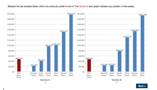
1    Introduction

Economists have long recognized that individuals incorporate others’ payoffs into their own
utility. This insight has given rise to a rich theoretical and experimental literature to better
understand the structure of individuals’ distributional preferences. Economists’ interest in
the topic is not merely academic — models of distributional preferences can help inform our
understanding of support for redistributive policies, political preferences, and the provision
of public goods. Much of the emphasis has been on testing various models of inequality aver-
sion. Many of these models assume functional forms in which the incomes of others matter
only in aggregate (as in, for example, Bolton and Ockenfels (2000)), or which add the possi-
bility that individuals try to help the worst-off person (as in Rawlsian preferences, explored
in Charness and Rabin (2002) and Engelmann and Strobel (2004)). Fehr and Schmidt (1999)
allow the disutility created by income gaps to depend on whether the gaps are disadvanta-
geous (resulting from incomes above the individual) or advantageous (resulting from incomes
below the individual), but within these two groupings income differences are just aggregated
to total disadvantageous and advantageous inequality.
    These models have performed well in experimental tests in which the decision-maker di-
vides earnings between herself and a single recipient or pair of recipients. But relatively little
work has explored their predictions in larger groups that may have more direct analogs in
the real world. To this end, we devise a simple experiment that allows subjects to express,
via revealed preference, their concern for inequality at different points in the income distri-
bution relative to their own. As a result, we may distinguish the extent to which subjects
place equal weight on the income gaps between themselves and all other individuals above
them (as in the most literal interpretation of Fehr and Schmidt (1999)) or if the incomes
of people in certain positions (e.g., the very top) in the income distribution appear to place
higher weight on their own utility. Similarly, we can test whether all advantageous income
gaps between oneself and those below carry equal weight.
    Specifically, we conduct a set of experiments via Mechanical Turk (MTurk) in which
each subject is confronted with a choice between two hypothetical societies A and B, each
with a different income distribution. In most versions of the experiment, each distribution is
comprised of seven individuals, including the subject herself. The two societies have differ-
ent income distributions, generated by taking independent draws from the same underlying
process. The data generating processes are designed to be reflective of the rough level of
prosperity in the United States, but to have some tilt toward the upper right tail, given
distributional preferences over this group will have the largest tax implications as a result of
their disproportionate share of income. For example, a typical distribution would be {$10,934,

                                                1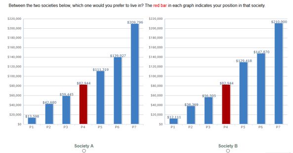
$28,102, $62,275, $92,479, $107,973, $151,869, $188,371}). By construction, in most variants,
the subject’s own income is held constant in Societies A and B (e.g., if she were the fourth-
ranked person in the given example, her income would be $92,479 and have a rank of four
in both distributions, whereas the other values would vary, independently sampled from the
given generating process). We make this choice to emphasize the role of others’ payoffs in
choosing distributional outcomes. Our design allows us to distinguish, for example, whether
individuals put more weight on reducing inequality at extreme income levels, or focus on
inequality nearer to the subject’s own income.
    Our first set of results does not explicitly consider the position of the subject herself, but
focuses instead on whether certain positions – most obviously the highest- and lowest-ranked
ones – play a particularly prominent role in subjects’ choices. We find a very robust emphasis
on reducing extreme inequality. Consistent with Rawlsian preferences and the results in
Charness and Rabin (2002) for two- and three-subject settings, subjects are significantly
more likely to select the distribution that raises the bottom individual’s income. This effect
is very large: a subject is about 30 percentage points more likely to select the distribution in
which the least well-off individual’s income is higher. More novel, we also find a robust and
quantitatively important emphasis on lowering the income of the individual in the highest
position in the distribution—subjects are more than ten percentage points more likely to
select the distribution with a lower income in the top position, all else equal. Apart from the
top and bottom incomes, no other absolute position has any impact on subjects’ decisions.
    In our second set of results, we define others’ positions in a relative sense: one position
above the subject, one below the subject, and so forth. We observe a large and significant
desire to reduce the income of the individual in the position directly above the subject’s own
income. In fact, this effect is comparable in magnitude to subjects’ preference for lowering
the income of the individual at the highest position in the distribution. By contrast, the
income two positions above her has no impact on the choice of distribution, and we can
reject at high levels of precision that these two effects are of equal magnitude. Such a result
is inconsistent with a general desire to reduce inequality.
    To organize our findings, we introduce the distinction between locally competitive versus
topmost competitive preferences to reflect our subjects’ particular focus on incomes very close
to their own as well as those at the top tail of the distribution. This framing can provide some
(parsimonious) guidance on the weights that individuals place on inequalities at particular
ranks in the income distribution, thereby enriching models of inequality aversion that are
standard in the literature. In particular, we can reject that individuals treat disadvantageous
income gaps symmetrically: instead we show that the immediate income gap between the
subject and the person right above her as well as the income gap between her and the richest

                                                2
person matter more than all other disadvantageous gaps. Similarly, we can reject that all
advantageous inequality is equal: instead, the advantageous inequality between the subject
and the worst-off person appears to differentially reduce utility.
Our framework may also help to reconcile some attitudes toward inequality that are
harder to explain with standard models. For example, consideration of local versus topmost
competitiveness is consistent with the popular outrage over the high incomes of the top one
percent. It can similarly explain why people care about “keeping up with the Jones” while
at the same time ignoring the somewhat more prosperous Johnsons.1
In the year following our initial pair of experiments (conducted in September, 2013), we
ran a number of additional “sessions” (given we use MTurk and not a true lab, “sessions” is a
slight abuse of the language, but by “session” we mean separate MTurk surveys administered
at particulars dates and times) that subjected our analysis to a wide range of robustness
checks. We allowed the subject’s own income to differ across the two distributions, varied the
generating processes to create distributions with higher levels of inequality, and increased
the number of individuals in each “society” to nine. We also varied the way that the distri-
butions were presented to subjects, pulling the bar representing the subject’s own income
away from those representing the incomes of others. Up to this point, all experiments con-
fronted subjects with hypothetical choices between pairs of income distributions. In our final
variant, we ran a real-stakes version in which subjects were informed that, with ten percent
probability, their choice would be implemented for stakes equal to one ten-thousandth of the
income distributions presented, with randomly drawn MTurk workers as recipients. Thus,
for example, if an individual in a selected distribution was assigned an income of $140,000
and that distribution was selected for real payoffs, a random MTurk worker would receive
$14 as payment.
We find that subjects in every session tended to choose distributions that reduce the
income of the individual in the highest position (i.e., subjects always exhibit topmost com-
petitiveness) and increase the income of the individual in the lowest position. Evidence for
“locally competitive” preferences is also observed in every variant apart from the “real stakes”
session, where its measured effect is much weaker (and statistically insignificant). We return
to discuss some possible explanations for this pattern when we present our experimental
findings.
Our paper contributes most directly to the recent literature that aims to infer redistribu-
1 Forexample, Luttmer (2005) shows that within relatively small geographic units, average local
income negatively predicts individual well-being, holding one’s own income constant. As these units
are more economically homogeneous than the entire country, the result suggests that individuals
care about the incomes of those close to them in the distribution (though that interpretation is
confounded by geographic proximity).
3tive preferences via survey methods. These studies have generally been devised to better un-
derstand attitudes toward (and impediments to) inequality-reducing redistribution in general
(e.g., Kuziemko et al. (2015), Norton and Ariely (2011)), without exploring the particular
structure of these preferences.
More broadly, our work builds on the large body of research that aims to characterize
the nature of distributional preferences. In our experimental design, we attempt to bridge
social preferences as typically studied in small groups with small stakes to preferences over
more policy-relevant income distributions. The literature we build upon encompasses the
theoretical contributions referenced earlier, many of which have experimental components
to them involving just one or two recipients.2
Our paper joins a smaller literature on distributional preference experiments involving
large groups. These studies tend to impose a formulaic redistribution parameter such that all
poorer individuals are made better off and all richer individuals made worse off, potentially
subject to some efficiency loss (see, in particular, Durante et al. (2014), Ackert et al. (2007),
and Beckman et al. (2004)). While this has the advantage of mimicking the effects of taxation,
it does not allow these prior studies to separate subjects’ concerns for others’ incomes at
particular points in the distribution.3
As our subjects are in a sense acting as social planners (though they are “planning” a
society of which they are a member), our work relates to the optimal tax literature under
non-standard preferences (either of the social planner herself or of individuals in society).
Recently, several important contributions on the theory side of this question have emerged.
Saez and Stantcheva (2016) examines optimal tax outcomes when the social planner is loss-
averse, Farhi and Gabaix (2015) develops optimal tax formulae under a number of behavioral
anomalies (e.g., inattention and mental accounting), and Lockwood (2016) focuses on present
bias. Our approach, as in Charité et al. (2015a), who test whether social planners respect
2 See Kahneman et al. (1986) for the earliest dictator experiment and Forsythe et al. (1994)
for the first appearance of the standard dictator game. More recent research has explored how
dictators’ fairness principles are affected by considerations such as deservingness (e.g., Almas et
al. (2010), Krawczyk (2010)) and extrinsic versus intrinsic motivations (Cappelen et al. (2017)).
Recent research has also generalized the dictator framework to incorporate different prices of giving
to create a tradeoff between equality and efficiency (see Andreoni and Miller (2002) and Fisman
et al. (2007)). We see our work as extending this tradition to consider the more complex set of
tradeoffs that come with distributional choices involving multiple others.
3 While less directly related to distributive preferences, a recent paper examines decision-making
in groups far larger than those in typical experiments. Schumacher et al. (forthcoming) finds that
many subjects make welfare-decreasing decisions while acting as social planners for large (up to 32
individuals) groups in lab experiments, because subjects weigh a salient benefit for a minority of
the group as more important than a small cost for the majority of the group, even if the sum of
the costs is greater than the sum of the benefits.
4individuals’ reference points, is more experimental.4
The remainder of the paper is organized as follows. Section 2 develops a very simple
generalization of the Fehr-Schmidt model that we will use to guide our empirical analysis.
Section 3 describes the experimental design. Section 4 explains the data collection procedure.
Section 5 presents the results from our main experiment as well as the follow-up sessions.
Section 6 offers concluding thoughts and suggestions for future work.
2 Standard models of distributional preferences
In this section, we summarize the classic inequality aversion model of Fehr and Schmidt
(1999), and also present a more flexible (though less parsimonious) version that will serve
as a point of departure for our empirical exercise.
We begin with the Fehr-Schmidt model. Consider a society of n individuals and a vector
of payoffs x = (x1 , ..., xn ); the utility function of individual i is then given by:
αi X βi X
Ui (x) = xi − max {xj − xi , 0} − max {xi − xj , 0} , (1)
n−1 n−1
where αi is individual i’s aversion to disadvantageous inequality and βi is his aversion to
advantageous inequality. The model assumes 0 ≤ βi < 1 and αi ≥ βi . These conditions
imply that individuals do not like advantageous or disadvantageous inequality (αi , βi ≥ 0),
but that they are not willing to reduce own-income in order to reduce inequality (βi < 1),
holding others’ incomes constant. The second assumption implies additionally that players
dislike falling behind more than they dislike being ahead of others.
In our setting, in which own-income is held constant (though we relax this constraint
in one experimental session), this model predicts that subjects will choose the distribution
that minimizes the aggregate payoff differences relative to others, with a greater weight on
4 In
comparing our results from hypothetical and real-stakes settings, we also contribute to a small
literature that seeks to test whether non-incentivized results generalize to incentivized settings. In
general, earlier research on this topic has found mixed results. Camerer and Hogarth (1999) perform
a meta-analysis of 74 studies that either have no, low or high-powered incentives. They find that
the effect of real stakes depends on the experimental task. Beattie and Loomes (1997) compare
three payment schemes: hypothetical, randomly picking one of several questions for payment, and
paying out for each question. They find that choices involving pair-wise comparisons of lotteries are
not affected by payment (although subjects are less likely to violate expected utility theory over
complicated sequences of lotteries when they are paid for each question). By contrast, while our
pair-wise comparisons are not tests of rationality, we do find that payment matters for subjects’
decisions. Etchart-Vincent and l’Haridon (2011) find that hypothetical and incentivized choices do
not differ for the choice to bear risk in the loss domain, but that hypothetical choices in the gain
domain are more risk-seeking than incentivized choices (consistent with Holt and Laury (2002)).
5decreasing high incomes rather than increasing low incomes. However, the model makes no
distinction among all individuals above the subject’s income or all individuals below: all
αi βi
incomes within each group are given the same weight, n−1 or n−1 , respectively.5
Individual- or rank-specific specific comparisons can easily be embedded in the Fehr-
Schmidt model by allowing parameters to vary for each of the other individuals’ positions.
Without loss of generality, we order the vector of incomes x in increasing order, so that the
fully flexible Fehr-Schmidt model may be expressed as:
n i−1
1 X 1 X
Ui (x) = xi − αi,j (xj − xi ) − βi,j (xi − xj ) (2)
n − 1 j=i+1 n − 1 j=1
Our experimental design allows us to potentially estimate all of these individuals’ specific
weights (αi,j and βi,j ). If we allowed for a fully flexible specification, it would lead to a very
large number of parameters (since they potentially depend on where the subject is in the
income distribution). As a result, we will present a set of graphs at the beginning of Section
5 that displays each of these parameters. We then inspect the patterns to determine the
regression specifications that the data appear to suggest. While there is some subjectivity
in going from the patterns in the graphs to an explicit regression specification, we will be
aided in this endeavor by the fact that we observe very clear patterns in the data: subjects’
inequality aversion focuses on the top and bottom individuals’ incomes (captured by αi,n
and βi,1 respectively), and locally disadvantageous inequality aversion (captured by αi,i+1 ).
3 Experimental Design
The centerpiece of the survey presents each subject with a binary choice between two income
distributions, which are called “Society A” and “Society B.” The survey experiment begins
with the following initial instructions (or a close variant of them, depending on whether we
were running the main survey experiment or one of the modified versions that we ran to
explore the robustness of our various findings):
In each round you will see two graphs displayed on your screen. Each graph
represents a distribution of payoffs that you can choose to assign to yourself and
to the other participants in your group. In each round, you must decide which
distribution, Society A or Society B, you prefer.
5 Bolton and Ockenfels (2000) adopt an approach that similarly yields no prediction of either
locally or topmost competitive preferences, based on the utility function Ui (x) = U (xi , Pxixj )
6Subjects then completed a practice round, which was accompanied by the following in-
structions:
Two graphs are displayed below. Each graph represents a distribution of payoffs
that you can choose to assign to yourself and the other participants in your group.
The red bar in each graph indicates your position and payoff in the group. Please
select which distribution you prefer.
After completing the practice round, subjects confirmed that they had read and under-
stood the directions before completing the ten subsequent iterations that constitute the data
we use in our analysis (see the screenshot in Figure 1).6
In every iteration, the subject’s own position in the income distribution was selected
at random. Further, in each iteration, instructions were reprinted above the two graphs,
as shown in the screenshot. Following the last iteration, subjects completed a short survey
on their attitudes toward government redistribution, their political preferences and voting
decisions, and basic demographics like age, gender, and income.
We focus our presentation of the results from the initial pair of experimental sessions
that we conducted, on September 9th and September 17th , 2013. In both sessions, subjects
were presented with choices that took the precise form illustrated in Figure 1, differing only
in the process by which the income distribution values were generated.
The income values for these sessions were drawn from uniform distributions in each
of seven ranges: (a1 , b1 ), (a2 , b2 )...(a7 , b7 ), where the subscripts denote the position p ∈
{1, 2, ..., 7} in the distribution. Note that position, as we define it, is increasing in income, as
opposed to rank. We set bp = ap+1 , so that the union of the intervals is (a1 , b7 )\{b1 , b2 , ...., b6 }
(i.e., the full interval minus a subset of measure zero). The non-overlapping ranges ensure
that in no case can ranks change from Society A to Society B. As such, if the subject finds
herself in position 4 in Society A, she will be in position 4 in Society B. We made this choice
to simplify the setting: the person right above a subject may move closer or further away,
but the subject can never “leapfrog” over him (nor can the subject be leapfrogged by the
person directly below).
To probe robustness, in our main experimental sessions we vary how the ap and bp
values are set. In one case, which we term “Absolute Differences” (AD), the ranges were
kept constant, in $20,000 increments, beginning at $10,000 (i.e., 10,000–30,000, 30,000–
50,000. . . 130,000–150,000). To give some sense of where these values sit in the distribution
of U.S. pre-tax, pre-transfer income, the midpoint of the lowest interval is at roughly the
6 Subjects were additionally assured that all responses would remain anonymous.
724th percentile and the midpoint of the highest interval is at roughly the 94th.7 In the sec-
ond case, which we term “Percentage Differences” (PD), we keep the percentage increase
in a comparable range across positions in the income distribution, increasing the range by
$5,000 at each level (i.e., the ranges are 10,000–25,000, 25,000–45,000. . . 175,000–220,000).
As indicated in the instructions, the subject’s own income is presented in a different color in
both distributions, and in all cases the subject’s own income is identical in each distribution
to focus the decision-maker on inequality rather than own-income.
We conducted a number of variants on this basic design to probe the robustness of our re-
sults to different income distributions and ways of presenting them to subjects. These variants
allow own income to vary; provide an alternative presentation of the income distributions, to
ensure that the results are not driven by the particular manner in which income distributions
are presented; change the distribution from which the income values are drawn; and make
the experiment for “real money.” We describe these companion experiments in greater detail
after documenting the results of the main experiment.
Table A1 provides a full list of the treatments (the main experiments plus the companion
experiments) as well as the dates they were conducted.
The interested reader can take the full experiment online at nautech-clients.com/
tobin/survey12/. The version posted online is the “real stakes” session (described in detail
in Section 5.3; its instructions are virtually identical to those of the main experiment, with
the addition of a screen which explains how payoffs will be determined as a result of the
subject’s choices in the experiment).
4 Data Collection
Over the past few years, social scientists have increasingly used MTurk to perform exper-
iments and collect survey data (see Kuziemko et al., 2015 and papers cited therein for a
review). We registered as a requester and created a human intelligence task (HIT) titled
“5-10 Minute Survey About Income Preferences”.8 To limit selection bias while also giving
workers an honest description of the task, we provided a short, neutral description of the
HIT (“This survey is part of an academic research survey”) that could be viewed by workers
7 These percentiles are based on the 2016 CPS. The midpoint of the second interval is at roughly
the 52nd, that of the third at the 72nd, that of the fourth at the 82nd, that of the fifth at the 88th,
and that of the sixth at the 92nd. As noted in the introduction, we wanted distributions with some
skew to the right.
8 Two sessions of the survey were administered with small changes to the HIT title. One session
was run with the title “7-10 Minute Survey About Income Preferences”, and another was run with
the title “10 Minute Research Survey About Income Preferences”.
8before they signed up to participate. Compensation was set to $.50 which, given the median
completion time of seven minutes, works out to an hourly wage of $4.25. Though we cannot
find official data on average wages on MTurk, reading through worker forums suggests that
we are paying a generous wage (and indeed our posted surveys were always filled within a
short period of time).
Each worker logs in with an MTurk worker ID. We collected data over seven separate
sessions, dropping any worker who had taken a previous survey with the same ID so as to
gather a fresh sample each time (though our main results hold when we keep repeat-takers in
the sample, as we show later). The sessions differed in the way that the income distributions
were generated or presented, as detailed in the preceding section.
To limit heterogeneity of the sample, we collected all data on workdays during daylight
hours on the East Coast of the United States. Individuals were prompted for a response if they
tried to skip questions (to further discourage robots and inattentive respondents). We also
limited the survey’s availability to those with U.S. billing addresses and asked respondents
to confirm their residency in the United States. We further limit respondents to those with
positive ratings from at least 90 percent of past MTurk requesters. Basic cross-tabs of the
data are reassuring (for example, subjects who report Republican party affiliation are roughly
fifty percent richer than those who report Democratic affiliation).
We informed subjects upfront that the survey was part of an academic study. Given
academia’s left-wing reputation, one might worry that social-desirability bias would lead
subjects to give more pro-redistribution answers (see, e.g., Bernardi, 2006, Dalton and Or-
tegren, 2011). In our setting, such concerns may be limited, as earlier research suggests that
web-based surveys may be less prone to social desirability bias than traditional in-person
interviews (Kreuter et al., 2008). We further tried to mitigate any such concerns by em-
phasizing early in the survey instructions that we sought individuals’ genuine responses,
explaining that: “You are invited to participate in an opinion survey. There are no right or
wrong answers [emph. in original].”
We also asked respondents directly about whether they perceived some left-wing, right-
wing or other sort of bias in our survey, though we only thought to do so in the very last
experimental session (on August 7th, 2014, the session for “real stakes”). Nonetheless, results
from this session suggest very few respondents felt the survey was biased. Roughly 7.6 and 2.7
percent, respectively, said it was biased in a “politically liberal” or “politically conservative”
manner, another 2.7 percent said it was biased in some other manner, with the remaining 87
percent saying they did not detect any bias. While these cross-tabs cannot speak to whether
subjects were biased in some subconscious manner, we are somewhat reassured that social
desirability bias is unlikely to be large.
94.1 Data sample
Table 1 provides details on all MTurk workers from all sessions that we conducted, comparing
them to the (weighted) population of adults sampled in the 2014 General Social Survey.
Consistent with past work using MTurk, we find that younger, male, and college-educated
subjects are over-represented in our sample.9 Also consistent with prior work, household
incomes are relatively low among MTurk workers. On the social and political variables that
may directly relate to distributional preferences, our sample is more likely to have voted than
the average GSS respondent, and slightly more apt to believe that government should reduce
income differences through redistribution. Relatedly, MTurk subjects are also more likely to
believe that success is a matter of luck than hard work, relative to GSS respondents. In a
robustness check we present results reweighted to be reflective of the GSS population based
on age, gender, income, and belief that the government should reduce income differences.
Table 2 provides a longer list of covariates for the MTurk sample.
4.2 Notation and definitions
Before proceeding to our main specifications and results, it is useful to provide some notation
and define several terms to facilitate our exposition in the next section.
We define several variables that capture differences between the two income distributions.
Let IncomeD p be the income of the individual in position p = 1, . . . 7 in Society D ∈ {A, B}.
Recall that position is increasing in income, so the poorest person in a seven-person distri-
bution has position 1 and the richest person has position 7.
We define Dif f Incomep as the income for position p in Society B minus the income for
position p in Society A. The preferences described in Section 2 predict that subjects will
make decisions based on absolute difference in income for p in B versus A, so that Society
B is preferred to Society A if and only if:
7 pi −1
X X
αj,pi Dif f Incomej − βj,pi Dif f Incomej > 0 (3)
j=pi +1 j=1
As a specific example, consider the income distributions presented in Figure 1. The sub-
ject is in position 4, with income of $82,944, while the position 5 incomes are $111,319 and
$129,418 for Societies A and B respectively. Since the position 5 income is higher in Society
B than Society A, Dif f Income5 = 18, 099 > 0. To assess whether Society A is preferred to
9 Unfortunately
our post-experiment survey did not ask for respondents’ race, but other studies
have found that MTurk workers are less likely to be minorities than the U.S. average.
10Society B overall, we need to assign utility weights for each position in the case that indi-
vidual i is in position 4. Suppose, for example, that the weights for positions one through
three are 1/8, 1/4, 1/2 and for positions five through seven they are 1/2, 1/4, 1/8 (so that
inequality aversion decreases with distance from the subject in the distribution). Summing
over the differences in incomes for each position, weighted by their respective weights, we
find that the expression above sums to 8439.63 so that Ui (SocietyB) > Ui (SocietyA).
We also employ an alternative measure of differences in income inequality between the two
distributions that is not sensitive to the widely differing income ranges at different positions in
the distribution. Specifically, instead of Dif f Income, we look at a binary indicator variable
that captures simply whether the income for position p is higher in Society B than in Society
A. That is,
1 if IncomeB − IncomeA > 0
p p
SignIncomep =
0 otherwise.
Note that for expositional parsimony we engage in some abuse of notation by calling this
variable SignIncome, when in fact it takes values of 0 and 1, not -1 and 1.
Finally, given our interest in testing whether respondents focus on those closer to them
in the distribution, we also define measures that are relative to the subject’s own position.
We thus define, for subject in position p, Dif f Income+1 = Dif f Incomep+1 . So, in the
preceding example (illustrated in Figure 1), Dif f Income+1 = 18, 099. 10
Past work has found that subjects often try to maximize total surplus, so it is natural
to consider total income as a control in some specifications (though its introduction into the
Fehr-Schmidt model is not without complications—we return to this point below). We define
Dif f Surplus as the difference in total income of all individuals in Society B versus Society
A:
7
X 7
X
Dif f Surplus = IncomeB
r − IncomeA
r.
r=1 r=1
Similarly, we generate an indicator variable, SignSurplus, that denotes whether Society B
has greater aggregate income than Society A.
10 Wesimilarly define Dif f Income+2 = Dif f Incomep+2 , Dif f Income−1 = Dif f Incomep−1 ,
and Dif f Income−2 = Dif f Incomep−2 .
115 Results
We begin by presenting visual displays of the data to depict how subjects decide between the
two distributions, and then proceed to more formal regression results. We present an initial
set of results that mirror the fully flexible specification in equation (2), which we will use
in large part to motivate the more parsimonious specification that we present in our main
regression tables.
5.1 Graphical evidence
We begin by exploring how subjects’ decisions depend on income differences between the
two distributions, independent of the subject’s own position. In Figure 3 we show the results
from the following specification:
7
X
ChooseB
ik =α+ λq SignIncomeq,ik + Pik + ik , (4)
q=1
which includes seven fixed effects for the position held by i in decision k (Pik ). ChooseB ik is
an indicator variable for subject i in iteration k of the experiment choosing Society B, and
SignIncomeq,ik is an indicator variable for position q having a higher income value in Society
B. Each coefficient λq can be interpreted as the percentage point increase in likelihood that
the subject selects Society B if the income of position q is higher in B. We also graph 95
percent confidence intervals, using standard errors clustered by subject.
In general, inequality aversion will lead subjects to pick distributions in which low po-
sitions have relatively high incomes. The graph clearly indicates a concern for raising the
income of the poorest member of society: the probability of selecting Society B is nearly
30 percentage points higher if the income in its lowest position is higher than in Society
A. We also observe an important role for the highest income—subjects are more than 10
percentage points more likely to select Society B if its richest individual has a lower income.
For positions two through six, we observe precisely estimated zero coefficients indicating
that, on average, incomes in these positions had no effect on subjects’ decisions. Overall,
our findings indicate that models of inequality aversion may wish to account for extremes in
income—both rich and poor—and place less emphasis on intermediate incomes.
We next explore whether subjects’ choices are affected by incomes relative to their own,
as would be the case in standard models of inequality aversion. We do so by allowing the
coefficients in the preceding analysis to vary depending on the subject’s own position in the
distribution, so that for each p ∈ {1, 2, . . . , 7}, we estimate the following equation via OLS:
12X
ChoiceB
ik = α + ηqp SignIncomeq,ik + ik (5)
q6=p
The estimation in each case is for all decisions k made by subject i in which she was assigned
position p in the income distribution. Similar to the preceding figure, the ηqp coefficients
tell us whether subjects are more or less likely to choose a distribution that is favorable to
position q when subjects are themselves in position p.
We plot the estimated ηqp coefficients separately for each value of p, across the seven panels
of Figure 4. As expected given the patterns in Figure 3, regardless of assigned rank, for all
p > 1, η1p is large and positive, indicating that subjects in all positions put considerable
weight on raising the income of the least well off individual (recall, η1p is not defined for
p = 1). We similarly observe that for all p < 7 η7p is negative across all panels, indicating a
general desire to “soak the rich.”
The only other case for which we observe a significant deviation from zero across all panels
is for the position directly above the subject’s own. In every panel, the “one above” coefficient
is negative and significantly different from zero at the five-percent level. No other coefficient
in positions two through six is significant across all panels, regardless of its position relative
to the subject. To emphasize the importance that subjects place on “one above” incomes
in particular, in panels (a) - (d) we can compare concern for the incomes of those one and
two positions above the subject’s own. In each case, we observe that for each own-position
p p
p, ηp+1 < ηp+2 (significant at least at the ten-percent level in all cases). That is, subjects are
averse to picking the distribution in which the individual in position p+1 has a relatively high
income, whereas the incomes of individuals in position p + 2 are relatively unimportant. (In
p p
panel (e), we observe that ηp+1 > ηp+2 , but this comparison conflates the effects of topmost
and local competitiveness.)
Other than these patterns, which indicate aversion to inequality at the extremes as well
as local competitiveness, relative incomes in other positions are uncorrelated with subjects’
choices. This pattern is difficult to reconcile with standard models of distributional prefer-
ences that emphasize aggregate differences or raising only extremely low incomes.
5.2 Regression results
Motivated by the preceding results, we present our main regression estimates in the following
parsimonious specification.
+1 +2
ChooseB 1
ik = β1 Dif f Incomeik + β2 Dif f Incomeik + β3 Dif f Incomeik
(6)
+β4 Dif f Income7ik + λXik + eik ,
13where Xik are covariates related to subject i or iteration k (e.g., subject fixed effects, itera-
tion fixed effects), which we vary to probe robustness. This specification focuses our analysis
on the patterns that emerged in the previous section, allowing us to explore the robustness
of inequality aversion toward top, bottom, and “one above” incomes across a range of speci-
fications (we include Dif f Income+2 to ensure that, in looking at “just above” incomes, we
distinguish local competition from general aversion to disadvantageous inequality). For these
analyses, we pool all decisions in which subjects held positions two through five, so that all
covariates are defined. Recall that we pool the first two experimental sessions, which consti-
tute the “baseline” experiment before we explore variants of the experiment. Throughout,
monetary values are expressed in units of $10, 000 to make the output tables more readable.
The coefficient on Dif f Income1 , for example, may be interpreted as the percentage point
increase in the probability of selecting Society B if the income of the poorest individual in
Society B increases by $10, 000 relative to the income of the poorest individual in Society A.
We present the results from this specification in Table 3. In column (1) we show the
results including the set of Dif f Income variables. The coefficients on Dif f Income1 and
Dif f Income7 are positive and negative, respectively, and both highly significant (p < 0.0001
in both cases). The coefficient on Dif f Income1 is 0.195, implying that a one standard devi-
ation increase in Dif f Income1 (0.688) leads to a 13.4 percentage point greater probability
that a subject selects Society B. The coefficient on Dif f Income7 , −0.0426, implies that
a one standard deviation increase in Dif f Income7 (1.231) leads to a 5.2 percentage point
lower probability that a subject selects Society B. We also find a strong local competition
effect: we estimate that β1 = −0.0371, whereas β2 = −0.000224. The difference is significant
at the one percent level.
In column (2) we include 10 question-order (iteration) fixed effects, which has little effect
on our estimates of the coefficients on the Dif f Income variables. Column (3) includes fixed
effects for the subject’s position in the income distribution. Column (4) excludes subjects
who completed the experiment very rapidly (less than 4 minutes). In all cases, the coefficients
on the Dif f Income variables are virtually unchanged.
In Appendix Table A2 we present results that reweight observations to be reflective of the
GSS population based on age, gender, income, and belief that the government should reduce
income differences. Results remain unchanged. While our preferred sample drops anyone in
the second session who already took the survey experiment in the first session, Appendix
Table A3 shows the results are robust to keeping these repeat-takers.
As Engelmann (2012) emphasizes, introducing a surplus term into the standard Fehr-
Schmidt model makes the coefficients difficult to interpret. For example, suppose we con-
trol for the change in total surplus in equation 6. Then, the effects of Dif f Income1 ,
14Dif f Income7 and Dif f Surplus could be re-interpreted as the effects of Dif f Income1 ,
Dif f Income7 and the total change in all other positions (as p Dif f Incomep = Dif f Surplus).
P
Put differently, holding Dif f Surplus constant (as we implicitly do when we control for it)
0
while increasing Dif f Incomep requires that some Dif f Incomep for p0 6= p must decrease.
Nonetheless, for the sake of completeness, we include the change in surplus in Appendix
Table A4. Our coefficients of interests remain unchanged. In particular, the coefficient on
Dif f Income1 barely falls, suggesting that little of the observed preference for raising the
income of the poorest person is explained by a desire to raise total surplus.
In a similar vein, we include the difference in Gini coefficients between the two distri-
butions as a control in Appendix Table A5, to ensure that the emphasis we document over
Dif f Income1 , Dif f Income7 , and Dif f Income+1 are distinguishable from a general dis-
taste for inequality. Again, we find that the coefficients on our variables of interest are largely
unchanged.
In Table 4 we repeat our analyses from Table 3, replacing the Dif f Income variables with
SignIncome variables (recall, a dummy for whether a given value in Distribution B is larger
than that in A). The results are qualitatively similar, but are more readily interpretable.
Consider the estimates in column (1). The coefficients on SignIncome1 , SignIncome7 , and
SignIncome+1 are 0.299, −0.107, and −0.0873 respectively (all significant at the one-percent
level), whereas the coefficient on SignIncome+2 is very close to zero. These results indicate
that a subject is nearly thirty percentage points more likely to select Society B if the income
of the poorest individual in that distribution is higher than the income of the poorest indi-
vidual in Society A. The coefficient estimates also indicate a significant concern for reducing
the incomes of individuals in the highest position and those in the position immediately
above the subject’s own. These latter two effects are of comparable magnitudes, and about
a third as large as the effect of the poorest individual’s income.
5.3 Results from companion experiments
So far we have shown that the results from our main experimental sessions are robust to a
wide range of specifications. We now document the results from the companion experiments
mentioned earlier to assess the robustness of our results to changing various aspects of the
experimental design.
After our two main experimental sessions, we conducted six additional experiments that
significantly changed some property of the original experiment.
1. The OV (“own variation”) experiment. This experiment allows the subject’s own in-
come to vary between distributions A and B. However, in both distributions he is in
15the same rank.
2. The NP (“nine player”) experiment. This experiment tests whether the main results are
robust to increasing the number of members in each distribution. For this experiment,
we begin with an interval of $10,000-$20,000, with the increment increasing by $4,000
for each interval, so that $202,000-$244,000 is the highest interval.
3. The HI (’“high inequality”) experiment. In the “high inequality” version, the lowest
income range was $10,000-$15,000, with the income ranges increasing by $10,000 at
each increment (so the top range was $190,000-$255,000).
4. The VI (“very high inequality”) experiment. In the “very high inequality” version, the
income ranges increased by $15,000 at each increment (so the top range was $265,000-
$360,000).
5. The AF (“alternative framing”) experiment. In this version, we provide an alternative
presentation of the data, with the subject’s own income presented to the far left of each
panel in every decision. See Figure 2. The purpose of this version of the experiment was
specifically to explore whether the local competition effect was attenuated by drawing
subjects’ attention away from the area of the graph immediately around their own
incomes.
6. The RS (“real stakes”) experiment. In this version, subjects were informed that, with
10 percent probability, one of their rounds would be implemented for a scaled down
version (with each value divided by 10, 000) of the chosen income distribution.
In Table 5 we repeat the specification from column (1) of Table 3 for these companion
experiments. (For completeness, a full set of results paralleling those presented in Table 3 are
available for each additional session in a series of Appendix tables.) The first two columns
in fact show the results from our main sample, but separately by session: first the “absolute
differences” session and then the “percentage differences” session. We show these results to
ensure that the results we report in Table 3 are not driven by just one of the two sessions.
Across all sessions, the coefficients on Dif f Income1 and Dif f Income7 are quite stable,
indicating that aversion to inequality at both the high and low extremes of the income
distribution is robust to the type of distribution, its presentation, as well as the introduction
of payoff consequences for subjects’ choices. Note that these effects are somewhat smaller in
column (3), suggesting that variation in own income crowds out interest in other aspects of
the distribution (and, not surprisingly, the R-squared term in this column is much larger, as
own income has very large predictive power).
16Our estimate of local competitiveness, as captured by β1 − β2 , is consistently negative
and significantly different from zero in the sessions that allow the subject’s own income to
vary (column 3), increase the number of players to nine (column 4, in which case topmost
inequality aversion is captured by Dif f Income9 ), vary the extent of inequality (columns 5
and 6), and present the distributions using an alternative formatting in which the subject’s
own income was placed separately at the left side of each distribution (column 7).
In general, framing effects are always a concern in a setting such as ours. Our distribu-
tions confront subjects with a good deal of information, leading to concerns that cognitively
overloaded subjects will focus on particularly salient parts of the distribution—the extremes
and those very close to them. Most compellingly, we find the robustness to the “alterna-
tive framing” (AF) variant to be encouraging evidence that concern for immediate income
neighbors does does not merely capture salience: in the AF session, the placement of the
red bar indicating own income would seem to distract attention from the “local” part of the
distribution, yet we find that subjects still lower the income of the individual above them.
Similarly, the “nine player” (NP) variant should lead to even more overload, as we have
increased the population of the distribution by over one-fourth. If information overload were
driving our results, we might expect to see larger coefficients on our variables of interest
in this session. Instead, we see that for the top and bottom incomes, the coefficients in the
NP session fall in the middle of the range defined by the full set of experiments (while the
local competition effect is on the larger side, the second largest of the eight sessions). Our
takeaway is that changing the amount of information confronting subjects as well as the way
it this information was presented has little effect on the overall patterns we observe in our
data.
5.4 Understanding differences in the real-stakes versus hypothetical sessions
Our three major results—top- and bottom-most inequality aversion and local competition—
replicate in seven of the eight sessions, and top- and bottom-most inequality aversion replicate
in all eight sessions. However, we find a weakened local competition effect in the real stakes
session (column 8). Individuals are still more likely to choose the distribution with the lower
income for the person directly above, though this result is no longer significant. Moreover,
when we compare this coefficient to that of the person two positions above, the difference,
while still of the predicted sign, is much smaller in magnitude and no longer significant.
The prior literature provides little guidance on this matter. Camerer and Hogarth (1999),
in particular, provide a meta-analysis of 74 studies that have no, low or high-powered in-
centives. They find that the effect of real stakes depends on the experimental task.11 None
11 Some more recent experiments since the meta-analysis was published focus specifically on
17of these experiments, however, concern the types of distributive principles that we explore
here. Moreover, we are also intentionally evoking the actual income distribution, which most
experiments do not do. The only redistribution experiment we know of that compares hy-
pothetical and real stakes is Charité et al. (2015b), who find similar results in a modified
dictator game with and without real stakes, though that experiment did not try to frame
outcomes in terms of actual, real-world income distributions.
The differing results across real stakes versus hypothetical treatments potentially raise
deeper methodological questions on the measurement of distributional preferences in lab
experiments. In particular, we are interested in studying distributional preferences over total
income or wealth, so that it is naturally impossible to implement subjects’ choices in practice.
As a result, when we impose payoff consequences we may substantively shift the distributive
principles that subjects invoke in making their decisions. That is, subjects may have in
mind the fairness principles toward a society’s income distribution overall when making
choices without direct payoff consequences. But when they are told that some specific, rather
1
arbitrary handful of actual people (those MTurk workers we are rewarding with 10,000 of
these “real-world” income values) will experience these payoffs, they may invoke different
principles.
It is also possible that individuals consider general-equilibrium effects when they think of
society’s income distribution. For example, the local competition effect could, in theory, be
driven by worries that if individuals slightly richer than oneself become even richer, goods
one is most likely to purchase become more expensive via increased demand. (Obviously,
general-equilibrium effects are negligible when only seven people are affected.)
Another challenge in applying results from small-stakes lab experiments to preferences
about society’s income distribution is that marginal utility of income enters more into the
latter framing than in the former. In the classic inequality-aversion set up, utility is linear in
own-income, an approximation that is likely innocuous for the small-stakes settings in which
it is typically tested.12 If subjects were highly sensitive to concerns about the diminishing
marginal utility of a dollar, we might expect that the coefficients on the tail incomes in the
“real stakes” version to be smaller in magnitude than in the other sessions (since the amount
of money involved would have trivial effects on the marginal utility of income in the “real
comparing behavior with and without payoff consequences, but again find mixed results. Further,
none of these recent studies invokes the sort of distributive concerns that are our focus in this
paper. See, for example, Etchart-Vincent and l’Haridon (2011) and Beattie and Loomes (1997).
12 It has been observed, however, that lab subjects may behave as if variation in small stakes
lead to diminishing marginal utility of money. See Rabin (2000), who attribute the large extent
of apparent risk-aversion that subjects display in choosing whether to participate in lotteries to
loss-aversion.
18stakes” version, but potentially large effects in the others). Comparing the “real stakes”
session to the other versions in Table 5 the coefficients on the top and bottom incomes are
generally quite similar (the coefficients found in the “real stakes” version are roughly at
the midpoint of the range formed by the full set of sessions). So, taken literally, our results
seem to suggest that these concerns were not paramount to our subjects. However, we find
this distinction (between true inequality aversion and beliefs about the diminishing marginal
utility of money) to be a very interesting question for future work.
Our paper has certainly not bridged the gap between distributive preferences over the
actual income distribution and those that can be tested in a real stakes setting (which will
naturally involve small stakes), but we hope that our findings provide a starting point for
future experiments that, like ours, attempt to further our understanding of both sets of
preferences.
5.5 Heterogeneity in Distributional Preferences
In our final set of analyses, we explore the extent to which our estimated effects from equa-
tion (6) vary systematically with political or self-stated distributional preferences, using our
main sample. In columns (1) and (2) of Table 6, we compare the decisions of self-identified
Democrats and Republicans (many subjects identified as independents, which is why the
total sample is smaller). We conjecture that, given the Republican Party platform in recent
decades of lowering taxes, its supporters will be less apt to choose distributions that reduce
inequality. Consistent with this view, we find that Republicans are less likely to choose dis-
tributions with lower incomes in the top position (i.e., the coefficient on Dif f Income7 is
less negative in column (2) than in column (1)). Similarly, Republicans are less likely to
select distributions with higher incomes in the lowest position. But we observe no difference
between the two subsamples in their attitudes toward incomes of those directly above them
— in both instances we observe a strong local competition effect.
In columns (3) and (4) we divide the sample based on responses to the question, “Do
you feel that the distribution of income and wealth in the U.S. today is fair or should be
more evenly distributed among a larger portion of the population?” Those in col. (3) take
the more redistributive position that income should be more evenly divided, whereas those
in col. (4) take the position that redistribution is not needed. In general, this cut of the data
reveals starker differences in preferences than we saw in the first two columns. The coefficient
on the poorest person’s income is 67 percent larger for those in col. (3) than in col. (4). Even
more striking differences between the two groups emerge in how they view the income of the
richest person. For those who feel no more redistribution is needed in the U.S., the income
of the richest person has no predictive power over which distribution is chosen (though the
19You can also read