Distributional Preferences Explain Individual Behavior Across Games and Time
←
→
Page content transcription
If your browser does not render page correctly, please read the page content below
Distributional Preferences Explain Individual Behavior
                                       Across Games and Time

           Morten Hedegaard, Rudolf Kerschbamer, Daniel Müller and Jean-Robert Tyran*

                                                  May 24, 2021

                                                     Abstract

            We use a large and heterogeneous sample of the Danish population to investigate the importance
         of distributional preferences for behavior in a trust game and a public good game. We find robust
         evidence for the significant explanatory power of distributional preferences. In fact, compared to
         twenty-one covariates, distributional preferences turn out to be the single most important predictor
         of behavior. Specifically, subjects who reveal benevolence in the domain of advantageous inequality
         are more likely to pick the trustworthy action in the trust game and contribute more to the public
         good than other subjects. Since the experiments were spread out more than one year, our results
         suggest that there is a component of distributional preferences that is stable across games and over
         time.

         Keywords: Distributional preferences, social preferences, Equality-Equivalence Test, representa-
         tive online experiment, trust game, public goods game, dictator game.
         JEL classification: C72, C91, D64.

   *
       Hedegaard: University of Copenhagen, e-mail: morten.hedegaard@gmail.com. Kerschbamer: University of Inns-
bruck, e-mail: rudolf.kerschbamer@uibk.ac.at.    Müller: University of Munich, e-mail: daniel.mueller@econ.lmu.de.
Tyran: University of Vienna and University of Copenhagen, e-mail: jean-robert.tyran@univie.ac.at. We benefited from
discussion with Ingvild Almås, Björn Bartling, Yves Breitmoser, Adrian Bruhin, Linda Dezső, Anna Dreber Almenberg,
Ernst Fehr, Ben Greiner, Michael Pfaffermayr, Georg Sator and Roman Sheremeta as well as from comments at the
ESA in Berlin, the 2019 Thurgau Experimental Meeting and the 2019 Nordic Behavioral Economics Meeting in Kiel.
We thank an associate editor and two anonymous referees for their thoughtful comments. We also wish to thank Erik
Wengström and the rest of the iLEE team for providing data from the first wave of experiments in the iLEE as well as
Eva Gregersen, Nikolaos Korfiatis and Thomas Alexander Stephens for their support in conducting the experiment. We
gratefully acknowledge generous financial support from the Carlsberg Foundation and from the Austrian Science Fund
(FWF) through special research area grant SFB F63, as well as through grant numbers P22669, P26901, P27912 and
I2027-G16.

                                                          1
1        Introduction
While standard economic theory typically assumes that agents care solely about their own material
payoff, there is by now ample evidence that the payoff of other people matters to decision makers
as well. This finding has important implications for both economic theory and policy. For example,
to evaluate the acceptance of tax policy, distributional preferences have to be taken into account.
The emerging empirical evidence led to the development of new models of social preferences that aim
at improving the predictive power of standard economic theory.1 These models have subsequently
become highly influential. While in general there is mounting evidence that distributional preferences
matter in specific contexts, less is known about their predictive power across games and their stability
across time. The current paper sheds new light on this open question.
        In this paper, we elicit distributional preferences using the Equality-Equivalence Test (EET; Ker-
schbamer, 2015) in a large and heterogeneous sample of the Danish population. The experiment is
conducted online using the Internet Laboratory for Experimental Economics (iLEE) based at the
University of Copenhagen. In this panel, participants take part in several online experiments in four
different waves. We exploit this rich source of experimental and survey data to make two contributions
to the literature.
        First, and most importantly, we investigate the predictive power of distributional preferences for
behavior in two games – a binary trust game (TG) and a linear public goods game (PGG). All our em-
pirical tests for the explanatory power of distributional preferences follow the same general structure:
We first derive individual-level point predictions from elicited preferences (and the beliefs about the
contributions of others in case of the PGG) using a social utility function along the lines of Fehr and
Schmidt (1999) and Charness and Rabin (2002). In addition, we derive necessary conditions for the
choices of subjects to depart from the selfish benchmark. In particular, we find that benevolence in
the domain of advantageous inequality is a necessary (but not sufficient) condition for the trustworthy
choice in the TG and a positive contribution in the PGG. We then show that (i) actual behavior
correlates with point predictions and (ii) subjects classified as benevolent when ahead are more likely
to pick the trustworthy option in the TG and contribute more in the PGG, even after controlling
for detailed measures of socio-economics, personality, cognitive ability and attitudes. A dominance
analysis (Azen and Budescu, 2003) shows that distributional preferences are the single most important
predictor of behavior across games. Our results highlight that taking distributional preferences into
account improves the predictive power of economic theory.
        Second, we provide evidence on the distribution of social preferences in the Danish population
and hence contribute to the discussion on the heterogeneity of these preferences. We document that
the empirically most frequent preference type is (with roughly a third of the population) altruistic.
Subjects are classified as altruistic if they are willing to give up own income to increase another
    1
        See for example Fehr and Schmidt (1999), Bolton and Ockenfels (2000), Fehr and Fischbacher (2002), Charness
and Rabin (2002) and Engelmann and Strobel (2004). We use the terms “distributional” and “social” preferences
interchangeably. Distributional preferences explain, for instance, bargaining behavior (De Bruyn and Bolton, 2008),
donations to charities (Derin-Güre and Uler, 2010; Kamas and Preston, 2015), voting decisions (Tyran and Sausgruber,
2006; Höchtl, Sausgruber, and Tyran, 2012; Paetzel, Sausgruber, and Traub, 2014; Fisman, Jakiela, and Kariv, 2017;
Kerschbamer and Müller, 2020), as well as competitive behavior (Balafoutas, Kerschbamer, and Sutter, 2012).

                                                          2
person’s income both when their income is higher and when it is lower than that of another person.
Around a quarter of subjects (23 percent) act in a way that is consistent with inequality aversion –
they reveal benevolence when ahead and malevolence when behind; a fifth (20 percent) behaves in a
selfish manner; and 14 percent are classified as having maximin preferences – they reveal benevolence
when ahead and neutrality when behind. In total, these four types make up 90 percent of our sample.
Thus, while the EET provides a comprehensive framework with nine social preference types, only four
of these are empirically relevant in our sample.2
We make these two advances by using state-of-the-art experimental methodology and high-quality
empirical data. Concerning methodology, we use the EET which delivers a parsimonious, nonparamet-
ric, comprehensive and mutually exclusive classification of individuals into distributional preference
types. Intuitively speaking, the test elicits the slope of an indifference curve when trading off income
for oneself versus income for another person. The EET delivers two measures of preference intensity –
the x-score and the y-score – which can easily be mapped into the two parameters of a piecewise-linear
utility function à la Fehr and Schmidt (1999) or Charness and Rabin (2002). This mapping – plus
the fact that we elicit beliefs about the contributions of others in the case of the PGG – allows us to
calculate individual-level predictions of behavior for both the TG and the PGG. Moreover, the EET
allows us to elicit the benevolence of the decision maker in the domain of advantageous as well as
disadvantageous inequality in a straightforward manner in one experimental framework. We consider
this property a distinct advantage relative to previous studies as in the EET preferences are unlikely
to be contaminated by strategic motives such as reciprocity. Moreover, our empirical implementation
of the EET delivers a credible measure of confusion (more than one switching point in the X- or the
Y-list) that most existing studies do not deliver (an exception is Blanco, Engelmann and Normann,
2011, who also observe multiple switch points and perform various robustness checks for different ways
of dealing with multiple switchers). We conduct several robustness checks to ensure that our results
are not driven by errors in decision making.3 In particular, we estimate a finite-mixture model of the
four most prevalent types and use posterior probabilities to classify the inconsistent participants into
their most likely types. Our conclusions remain unchallenged by this exercise.
Overall, our findings demonstrate that distributional preferences matter for behavior in experi-
mental games and that taking them into account is important to improve the empirical realism of
economic models. The results in this paper contrasts with previous experimental evidence that ques-
tioned the predictive power of social preference models (Blanco, Engelmann, and Normann, 2011).
Our paper also highlights the advantages of using the EET over a standard dictator game (DG), which
has frequently been used as a proxy for distributional preferences, in interpreting strategic decision
making. The reason is that behavior in the games studied here does not correlate well with behavior
in the DG, see Appendix A.2 for details, but does correlate well with decisions in the EET.
The paper is organized as follows. Section 2 discusses related literature. Section 3 provides a
short introduction to the EET and informs about the online experiments conducted in the iLEE.
2
This finding resonates well with that of Kerschbamer and Müller (2020) who reach similar conclusions in a sample
of the German population. However, they find a larger proportion of inequality-averse subjects than in Denmark. This
raises intriguing questions about the origins and international differences of social preferences.
3
Andersson, Holm, Tyran, and Wengström (2016), for example, find evidence that errors in decision making can lead
to a spurious correlation between cognitive ability and risk preferences.
3Section 4 discusses the distribution of social preferences in Denmark. Sections 5 and 6 present the
evidence for the predictive power of distributional preferences for behavior in the TG and the PGG,
respectively. Section 7 concludes. In the appendix we present additional descriptive statistics, sev-
eral robustness checks including a finite-mixture model, and a detailed description of the experiment
including instructions.
2 Related Literature
Our paper contributes to an ongoing debate on the relevance of social preferences for behavior in
experimental games. In general, it is fair to say that the literature has not yet reached a clear verdict
on this question.
One of the most prominent contributions is Blanco, Engelmann, and Normann (2011). The authors
study behavior in four games – an ultimatum game (UG), a modified dictator game (DG), a sequential
prisoner’s dilemma game (PDG) and a public goods game (PGG) – with the aim of testing the Fehr
and Schmidt (1999) model of inequality aversion. They use responder data from the UG to estimate
aversion to disadvantageous inequality and the data from the modified DG to estimate aversion to
advantageous inequality. The resulting measures are used to predict decisions in the other two games.
The authors find that the Fehr and Schmidt (1999) model has considerable predictive power at the
aggregate level but performs less well at the individual level.
There are other studies that reach similar conclusions to Blanco et al. (2011). Engelmann and
Strobel (2010) focus on the predictive power of inequality aversion for behavior in the moonlighting
game and do not find any significant correlations in situations where inequality aversion and reciprocity
make different predictions.4 Yamagishi et al. (2012) find that rejection of offers in the UG is not
correlated with behavior in other games, including a standard DG. See also Kümmerli et al. (2010),
Burton-Chellew and West (2013) and Capraro and Rand (2018) for similar claims.
Several papers find mixed evidence for the predictive power of social preferences for behavior
in experimental games. Teyssier (2012) studies the role of inequity aversion and risk preferences for
cooperative behavior in two versions of a PGG. She employs the same method to elicit inequity aversion
as Blanco et al. (2011) and finds that inequity aversion explains contributions in a sequential PGG,
but not in a simultaneous PGG. Dannenberg et al. (2007) classify subjects into Fehr-Schmidt and non-
Fehr-Schmidt types based on their choices in a DG and an UG. On the one hand, they find that the
composition of groups based on these social preferences significantly influences contribution behavior
in a PGG in the sense that inequality averse subjects contribute more. On the other hand, it turns out
that information about the players in the own group is required to raise contributions, such that “fair”
groups contribute more to the common good. Harbaugh and Krause (2000) find mixed evidence for the
correlation of behavior in a DG and a repeated PGG with children. In particular, there is a correlation
between DG behavior and behavior in the first round of the PGG in the expected direction, but no
strong correlation to behavior in the last round of the PGG. Finally, Dreber, Fudenberg, and Rand
(2014) examine whether giving in a standard DG explains cooperation in a repeated PD. They find
4
In the moonlighting game by Abbink, Irlenbusch, and Renner (2000) the first mover can give money to or take
money from the second mover, who can then either reward or punish the first mover.
4evidence for a correlation when no equilibrium involving cooperation exists, but not when cooperation
is an equilibrium.
Several studies have found evidence that distributional preferences predict behavior in games.
Most closely related to our work is Bruhin, Fehr, and Schunk (2019) who estimate a mixture model
of social preference types. Their model includes distributional as well as reciprocal concerns. They
find three preference types in a student sample: strong altruists, moderate altruists and a “behindness
averse” type. In addition to classifying subjects into types based on the posterior probabilities from
the mixture model, the authors show that the structural parameters from the mixture model predict
behavior in a TG and a ‘reward and punishment game’. Kamas and Preston (2012) elicit behavior in
a DG, an UG and a TG and conclude that their data offers “strong support” for social preferences
to matter across games. Yang, Onderstal, and Schram (2016) elicit the two parameters of the Fehr-
Schmidt model at the individual-level and find that these parameters matter in explaining choices in
a ‘production game’. Peysakhovich, Nowak, and Rand (2014) find evidence for a correlation of pro-
social behavior across five different games conducted 124 days apart, including a DG. They conclude
that there is a general and temporally stable component to pro-social behavior, which they dub the
“cooperative phenotype”.
Offerman, Sonnemans, and Schram (1996) and Murphy and Ackermann (2017) show that sub-
jects’ social value orientation predicts cooperativeness in a PGG, see also Yamagishi et al. (2013).
Hernandez-Lagos, Minor, and Sisak (2017) find that social preferences predict effort provision and
coordination in a lab experiment. Gächter, Nosenzo, and Sefton (2013) show that Fehr-Schmidt
preferences are better able to explain peer effects in a three-person UG than social norms. Holm
and Danielson (2005) find that behavior in the DG is significantly related to behavior in the TG in
Tanzania and in Sweden.
We shed new light on these mixed findings and make several contributions to the literature. First,
we use individual-level measures of distributional preferences to make point predictions of behavior
in other games which allows for a sharper test. This seemingly subtle issue is, we believe, important
and distinguishes the current paper from the rest of the literature (again, one exception is Blanco et
al. (2011) who also use individual-level measures of distributional preferences to make predictions;
however, since they do not elicit beliefs, they cannot make point predictions for the PGG): If one
does not measure distributional preferences, there is no way of telling whether they matter or not.
Also, the evidence presented in this paper shows that the preference elicitation needs to distinguish
between benevolence in the domain of advantageous and benevolence in the domain of disadvantageous
inequality. This is so, because (i) those inclinations are empirically uncorrelated and (ii) it is otherwise
mathematically impossible to calculate point predictions across games. Thus, empirical elicitation
procedures that do not distinguish these domains – like the Ring Test and the Circle Test developed
by Griesinger and Livingston (1973) and Liebrand (1984) and the basic version of the Social-Value-
Orientation Slider introduced by Murphy, Ackermann, and Handgraaf (2011) – are not suited to
study the question that the current paper tackles. Second, our results demonstrate that there is
a component to distributional preferences that is stable over longer periods of time because one
game was implemented one year prior to the other games. Third, we demonstrate the predictive
power of social preferences in a representative sample instead of a convenience sample of students.
5Our findings therefore suggest that distributional preferences can predict behavior not only among
possibly more highly educated student samples recruited for controlled laboratory experiments but also
in an online survey involving a random sample from the general population. Fourth, we demonstrate
that distributional preferences are the most important predictor of behavior relative to a large set of
potentially relevant covariates. This demonstration is particular powerful in a heterogeneous sample
which exhibits larger variation than convenience samples. Fifth, we find that while the EET predicts
well, the standard DG does not. Thus, this finding suggests that the EET is a more appropriate
measure of distributional preferences.
3 Experiments in the iLEE and the EET
This section first provides a short introduction to the Equality-Equivalence Test (EET) proposed
by Kerschbamer (2015) and then informs about the online experiments conducted in the internet
Laboratory for Experimental Economics (iLEE) that we exploit to gather our data.
3.1 The Equality-Equivalence Test
The EET is a price-list technique that aims at identifying the benevolence, neutrality or malevolence of
the decision maker towards an anonymous other subject (the recipient) in two domains of inequality –
the domain of advantageous inequality where the decision maker is ahead of the other person, and the
domain of disadvantageous inequality where the decision maker is behind. Depending on the revealed
benevolence, neutrality or malevolence of the decision maker in the two domains, the decision maker
is classified into one of nine social preference types – for instance, as altruistic if the decision maker
reveals benevolence towards the recipient in both domains, as inequality averse if the decision maker
reveals benevolence in the domain of advantageous and malevolence in the domain of disadvantageous
inequality and as selfish if the decision maker reveals neutrality in both domains. See Figure 1 for
details.5
More specifically, the EET exposes subjects to a number of binary choices between two income
distributions (m, o), where m (for “my”) stands for the own material payoff of the decision maker
while o (for “other”) stands for the material payoff of the other person. In each choice problem one
of the two alternatives consists of a symmetric reference allocation in which both subjects receive the
same material payoffs. In the version of the test we use (this version is displayed in Table 1 and
graphically illustrated in Figure 2), the symmetric reference allocation was set to 50 Danish Kroner
(Dkr; approximately 7 euros) for each person. The second allocation is always asymmetric. In half of
the binary choices (the advantageous inequality block – the Y-list) the decision maker gets more than
the recipient, in the other half (the disadvantageous inequality block – the X-list) the decision maker
always gets less. Within each of the two blocks the material payoff of the recipient in the asymmetric
allocation is held constant, while the material payoff of the decision maker increases monotonically
from one choice to the next.6 This design feature (together with the fact that the symmetric allocation
5
A positively (negatively) sloped indifference curve in a given domain corresponds to malevolence (benevolence) in
that domain, while a vertical segment corresponds to neutrality.
6
We varied the incremental change in m in the asymmetric allocation (the “step size”, which is constant in the basic
version of the test) so that it is small (2 DKr) close to the reference point but grows larger (up to 10 DKr) when moving
6remains the same in all choices) guarantees that a rational decision maker switches at most once from
the symmetric to the asymmetric allocation (and never in the other direction) within each block.7
As Kerschbamer (2015) shows, the two switching points of a subject can be used to construct a
two-dimensional index – the (x, y)-score – representing both archetype and intensity of distributional
concerns. A positive score corresponds to benevolence and a negative score to malevolence. The y-score
thereby refers to preferences in the domain of advantageous inequality and the x-score to preferences
in the domain of disadvantageous inequality. Moreover, a higher score means more benevolence. For
instance, a subject that switches from the symmetric to the asymmetric allocation in row 2 of the
X-list shown in Table 1 reveals more benevolence in the domain of disadvantageous inequality than a
subject who switches in row 3. This is so because the former subject reveals that it is willing to give
up at least 20 Dkr to increase the income of the recipient by 25 Dkr, while the latter subject reveals
that it is not willing to give up 20 Dkr to increase the income of the recipient by 25 Dkr, but would
be willing to give up 8 Dkr to do so. To account for the difference in benevolence, the EET assigns
an x-score of 3.5 to the former subject and an x-score of 2.5 to the latter. Suppose now a subject
switches from the symmetric to the asymmetric allocation in row 5 (row 6, respectively). This subject
reveals that it is not willing to give up 2 Dkr to increase (decrease) the material payoff of the recipient
by 25 Dkr, but is willing to do so if the change in the income of the recipient does not involve a cost
in own-money terms. The EET assigns to such a subject an x-score of 0.5 (-0.5, respectively), as the
subject reveals to be weakly benevolent (weakly malevolent, respectively). In the EET, the scores
+0.5 and -0.5 are interpreted as selfishness in the respective domains, as the subject has revealed that
it is not willing to give up 2 Dkr to change the income of the recipient by 25 Dkr.8
The EET provides several advantages over alternative approaches to elicit distributional prefer-
ences. First, it is derived from a small set of axioms on preferences. Thus, the conditions under
which the test holds are well-defined. Second, the same set of assumptions result in a well-delineated,
mutually-exclusive and comprehensive set of distributional types. Thus, the set of distributional types
tested for is not ad hoc but rather derived from assumptions about preferences. Third, the test is
non-parametric and hence does not rely on any functional form assumption. Fourth, the preferences
are elicited in an environment uncontaminated by intentions and beliefs – which is in contrast to large
parts of previous literature.
Given the direct relation of the current paper to the work by Blanco et al. (2011), it is instructive
to compare their elicitation procedures to the EET. To estimate the parameter of aversion against
advantageous inequality Blanco et al. use a technique that bears similarities to the EET. In terms
of Figure 2, Blanco et al.’s 20 binary decisions correspond to 20 points on the 45° line through the
positive orthant each compared to a single point that has exactly the same m as the rightmost point
on the 45° line but an o of zero. Thus, by observing the choices of a subject in the 20 binary decision
problems one can deduce the shape of the indifference curve through this latter point. While this is an
away from the reference point. This modification in comparison to the basic version of the test was made to increase the
power to discriminate between selfish and non-selfish (that is, benevolent or malevolent) behavior without increasing the
test size or decreasing the discriminatory power at the borders.
7
The rationality requirements underlying the EET are low. In terms of axioms on preferences the assumptions are
ordering (completeness and transitivity) and strict own-money monotonicity – see Kerschbamer (2015) for details.
8
In the EET, selfishness ‘has a sign’: A subject with a score of +0.5 reveals benevolence (and one with -0.5 reveals
malevolence) only in those decisions in which no own money is at stake.
7elegant procedure it has some disadvantages in comparison to the EET employed here, namely (i) that
the shape of the indifference curve can only be assessed for the domain of advantageous inequality;
and (ii) that positively sloped indifference curves in that domain cannot be identified correctly. To
estimate a subject’s parameter of aversion against disadvantageous inequality Blanco et al. (2011) use
data from second-mover behavior in the ultimatum game. A potential disadvantage of this approach
is that the second mover is likely to read first-mover intentions into observed first-mover choices.9
Figure 1: Indifference curves for the nine archetypes of distributional preferences.
The EET was part of wave 3 of the internet Laboratory for Experimental Economics (iLEE). The
procedures of the test were as follows. Participants were first explained the rules of the experiment.
See Section A.6 in the appendix for experimental instructions and A.7 for screenshots. Choices were
made one at the time on separate screens where decision makers choose between Left and Right before
moving on to the next choice. Once they have made all 14 choices, subjects saw a confirmation screen.
This screen provided an overview of the choices made by the subject in the EET with a horizontal
line separating the X- and the Y-list. The chosen distributions were color highlighted and decision
makers could go back and change their decisions as many times as they wished. Once they confirmed
their decisions, they moved on to the next experiment in the wave.
9
This should not be read as a critique of Blanco et al.’s (2011) approach. After all, the Fehr and Schmidt model
has been designed to explain behavior in strategic games and the ‘calibration’ of parameters with ultimatum game data
has been suggested by the authors of the original paper. A possible advantage of Blanco et al.’s approach (in terms of
explaining behavior in strategic games) is that it captures not only distributional preferences but also other forms of
other-regarding preferences (such as reciprocity motives, for instance).
8The X-list The Y-list
Left Right Left Right
m o m o m o m o
20 75 50 50 42 25 50 50
30 75 50 50 48 25 50 50
42 75 50 50 50 25 50 50
48 75 50 50 52 25 50 50
50 75 50 50 58 25 50 50
52 75 50 50 70 25 50 50
58 75 50 50 80 25 50 50
Table 1: The X- and the Y-list implemented in the iLEE. All numbers in Danish kroner.
Figure 2: Graphical illustration of the allocations.
We employed two conditions that relate to the roles and possible interaction of decision makers and
recipients. In the FixedRoles condition half of the participants were decision makers, the other half
were recipients. Roles were randomly assigned and revealed after participants read the instructions
but before any decisions were made. Decision makers then made their choices in the EET while
recipients made no decisions. At the very end of the experiment, each decision maker was randomly
assigned to a recipient and one randomly selected choice was then actually paid out in each pair.
In the RandomRoles condition all participants made choices as if they were decision makers. A
random draw determined ex-post which role each participant was paid for. Again, half of the subjects
received the decision maker role and half the recipient role, each subject in the decision maker role
was randomly assigned to one in the recipient role and one randomly selected choice was then actually
paid out. Instructions were kept as similar as possible across conditions and treatment allocation was
9random with one-third of participants in the FixedRoles condition and two-thirds in the RandomRoles
condition. We implemented these two conditions to explore whether the role assignment has an impact
on the elicited distributional type – which could potentially explain the conflicting evidence reported
in Section 2. Our ex-ante hypothesis in this regard was that the role assignment is of secondary
importance.
3.2 The Internet Laboratory for Experimental Economics
The experiment uses a “virtual lab” approach and is conducted using the platform of the internet
Laboratory for Experimental Economics (iLEE) at the University of Copenhagen, Denmark – see
Thöni, Tyran, and Wengström (2012). Subjects for the platform are recruited with the assistance
of the official statistics agency (Statistics Denmark) who selects a random sample from the general
population. The iLEE consists of four different waves, issued between May 2008 and June 2011.10
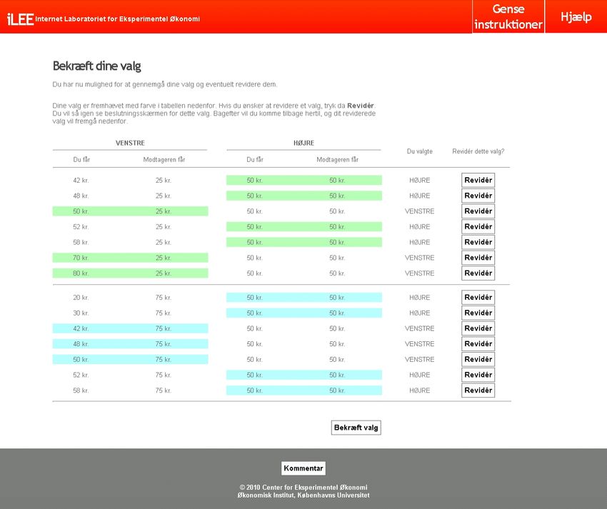
In the binary trust game (TG), which was part of wave three of iLEE in July 2010, each subject
makes two decisions, one in the role of the first mover and one in the role of the second mover. Subjects
were informed in the instructions that only one of the two decisions would actually be paid out. For
half of the subjects the first-mover decision was selected to be payoff relevant, for the other half the
second-mover decision was payoff relevant. The matching of subjects was random and one-to-one.
The first mover had to decide between in and out. Out implies payoffs of 50 Dkr and 20 Dkr for the
first and the second mover. In implies that the decision is passed on to the second mover. The second
mover then decides between betrayal and honor, which implements the payoff pair (20,90) or (80,40),
respectively. Here, we only consider the decisions of the second mover, as they are clearly distributive
in nature.
The linear public good game (PGG) was part of the first wave of the iLEE. In this experiment,
subjects are matched into groups of four. Each subject is endowed with Dkr 50 and decides how much
to contribute to a pool of common resources (the public good) and how much to keep for herself (the
private good). The total amount contributed by the group to the common pool is doubled and shared
equally among the group members (the marginal per capita return, MPCR, is hence equal to 0.5).
The PGG is played as a one-shot game. In this game, half of the participants were randomized into
a “give” frame and the other half into a “take” frame.11 While it is socially optimal that all group
members contribute the full endowment, individual income is maximized by contributing zero. After
the contribution decision, we elicit beliefs about the average contribution of the three other group
members incentivized using a quadratic scoring rule.
When analyzing the data, we include three different sets of control variables in our regressions, all
taken from the iLEE survey: First, the socio-demographic set consists of age; age squared; a gender
dummy; education (coded in four different categories); dummies for employed, retired, student and
self-employed status; income (coded in quartiles); and the number of hours worked per week. Second,
the personality and cognitive controls comprise the IQ score; the score from the cognitive reflection
10
More detailed information about the iLEE is presented in Section A.5 in the appendix. See also the web page
http://www.econ.ku.dk/cee/ilee/description/ for further information. On this web page one can also find comparisons
of the characteristics of the sample with those of the general Danish population.
11
The average contributions are in fact not influenced by this frame, but we nevertheless control for the frame in all
regressions. More details can be found in Fosgaard, Hansen, and Wengström (2019).
10test; and the Big-5 character traits. Third, the set of attitude controls consists of three different
variables indicating political preferences and trust. All these variables are explained in more detail in
Section A.5.
4 The Distribution of Social Preferences in Denmark
In total, 1067 participants took part in the experiment – with average earnings of 51.8 Dkr. From
these 1067 subjects, 885 played the role of a decision maker in the EET, while the rest was only
in the role of a recipient (in the FixedRole condition). The assumptions of ordering and strict m-
monotonicity imply that decision makers switch at most once from Right to Left (and never from Left
to Right) in each list of the EET. Of the n = 885 decision makers, 650 fulfill this rationality criterion
while 235 (27%) make choices that are not consistent with it.12 In the main analysis we focus on
the consistent decision makers. Later on, in the robustness section, we also estimate mixture models
and use posterior probabilities to classify inconsistent participants into one of the four main types.
Regarding the two payment protocols, we find very little evidence that these two payment protocols
cause differences in behavior. In particular, we do not find evidence that the number of consistent
subjects or the frequency of distributional types is affected. Appendix A.3 reports more details. In
the following, we therefore merge the data without using dummies for the protocols. The results with
the dummies are very similar and available upon request.
Table 2 displays the distribution of social preferences types in Denmark. The first column of
the table shows that, among the classified subjects, the empirically most frequent preference type is
(with roughly a third of the population) altruism. Subjects are classified as altruistic if they reveal
benevolence both when they are ahead and when they are behind. Around a quarter of subjects (23
percent) act in a way that is consistent with inequality aversion – they reveal benevolence when ahead
and malevolence when behind; a fifth (20 percent) behaves is a selfish manner – their behavior seems
to be unaffected by the material consequences for others, independently of whether they are ahead
or behind; and 14 percent are classified as having maximin preferences – they reveal benevolence
when ahead and neutrality when behind.13 In total, these four most prevalent types make up almost
90 percent of the sample. Of the remaining, less than six percent act in a way that is consistent
with envy and less than three percent are spiteful, while kiss-up, equality averse and kick-down each
account for only about one percent of the sample. Thus, while the EET provides a comprehensive
framework which allows for the distinction between nine social preference types, only five of these
12
This share is relatively large – compared to the 5% share reported by Kerschbamer (2015) for a standard lab
experiment based on a student subject pool, for instance. A possible reason for the large share of inconsistent subjects
is the heterogeneity and representativeness of the sample on which our study is based. Evidence in support of this
conjecture comes from an earlier wave of the iLEE: Andersson, Holm, Tyran, and Wengström (2016) report that 35% of
the sample had multiple switching points in a variation of the Holt and Laury (2002) risk attitudes elicitation procedure
– which is similar to the EET with regards to complexity.
13
For a two-player decision problem, the label “maximin” for a player who is benevolent towards a player with lower
payoff and neutral towards a player with higher payoff seems fine. However, we are later analyzing a game with four
players. In such a game benevolence towards players with lower payoffs and neutrality towards players with higher
payoffs is only consistent with maximin preferences if all players with lower payoffs have exactly the same low payoff.
Hence, a different term – ‘charitable’, for instance – seems more appropriate. To avoid the introduction of new names
for preference types, we stick to the term maximin throughout the paper.
11types attract more than 5% of our subjects.14 Figure 3 plots the distribution of social preference
types in our population in the (x, y) space. In this space, the x-score, measuring the benevolence of
the decision maker in the domain of disadvantageous inequality, is represented on the x-axis and the
y-score, measuring benevolence in the domain of advantageous inequality, is represented on the y-axis
(in both cases negative values mean malevolence, see Subsection 3.1 for details). The figure clearly
shows that there are pronounced mass points in the top-left corner (inequality-aversion) and in the
center (selfishness), and that there is a densely populated area of somewhat smaller mass points in
the positive orthant (with maximin covering the left-hand side of the area and altruism covering the
rest).
Types Distribution
Altruist 32.2
Inequality averse 23.2
Selfish 20.0
Maximin 13.7
Envious 5.5
Spiteful 2.6
Kiss-up 1.2
Equality averse 1.1
Kick-down 0.5
N 650
Table 2: Distribution of social preference types in percent.
5 Trust Game
We now turn to the assessment of the predictive power of distributional preferences across different
games. We first investigate how distributional preferences explain behavior in the binary TG. Section
6 then considers the linear PGG.
14
The share of inequality-averse subjects might seem rather high in comparison to the findings in Kritikos and Bolle
(2001), Charness and Rabin (2002) and Engelmann and Strobel (2004). A possible explanation is that the EET is biased
in the direction of detecting more inequality averse people – for instance, because the EET uses a symmetric reference
allocation that might act as an anchor. We are not convinced by this explanation for several reasons: First, when the
EET is employed in student samples, the fraction of inequality averse subjects is typically rather low – see Kerschbamer
(2015), Balafoutas et al. (2017) or Kerschbamer at al. (2019). Second, there are several recent papers that do not make
use of the EET and still find relatively large shares of inequality averse subjects – see Bruhin et al. (2019). Third, the
study by Krawczyk and Le Lec (2021) implements a variant of the EET with asymmetric reference points and detects
a similar fraction of inequality averse subjects as Kerschbamer (2015). Given all this evidence we consider it as more
plausible that differences in subject pools are responsible at least to large parts for the differences in results. See Fehr et
al. (2006) for experimental evidence indicating that students (especially students of economics) are less egalitarian and
more efficiency oriented than the rest of the population. See also the response by Engelmann and Strobel (2006) in the
same issue.
12Figure 3: Scatterplot of (x, y) scores.
5.1 Prediction for the TG
We first analyze the predictive power of distributional preferences for second-mover behavior in the
binary TG contained in wave 3 of the iLEE. A screenshot of the TG is shown in Figure 6 in the
appendix.
In order to make an individual-level prediction for our binary TG, we use the piecewise-linear
social utility function proposed by Fehr and Schmidt (1999), but lift their parameter restrictions. For
the two-agents case, the Fehr-Schmidt function reads:
(
(1 − σ)m + σo if m ≤ o
U (m, o) = (1)
(1 − ρ)m + ρo if m > o,
where m (for my) denotes again the income of the decision maker and o (for other’s) the income of the
second person and where σ and ρ are two parameters that determine the weight the decision maker
puts on the income of the other person when she is behind (m ≤ o) or ahead (m > o), respectively.15
To simplify the exposition, we assume in the main text that σ ≤ ρ < 1. The former inequality
means that the decision maker is more benevolent (less malevolent) in the domain of advantageous
than in the domain of disadvantageous inequality and it guarantees that indifference curves in the
(m, o)-space are convex.16 The latter inequality makes sure that the preferences of the decision maker
are monotone in the own material payoff.
15
Note that we use the parameters σ and ρ here (and not the conventional α and β) in order to make clear that we
do not make the usual assumptions about the values of the parameters, i.e. 0 ≤ β ≤ α.
16
The convexity assumption excludes three types of preferences (equality-averse, kiss-up and kick-down) and we will
discuss the prediction for these types in footnotes.
13A second mover in the TG faces the decision between betrayal and honor, implying the allocations
(20, 90) and (80, 40), respectively.17 Inserting these payoffs into (1), we see that the second mover
prefers (80, 40) over (20, 90) iff
(1 − σ)40 + σ80 ≥ (1 − ρ)90 + ρ20, (2)
which yields the prediction:
Prediction for the TG: Consider a binary TG, in which the second mover has the choice between
the payoff allocations (20, 90) and (80, 40). Suppose the second mover’s preferences are of the Fehr-
Schmidt form, but with parameters only restricted by σ ≤ ρ < 1. Then
if 4σ + 7ρ > 5 the second mover’s uniquely optimal move is to pick honor;
if 4σ + 7ρ = 5 the second mover is indifferent between betrayal and honor; and
if 4σ + 7ρ < 5 the second mover’s uniquely optimal move is to pick betrayal.
In our main analysis we test the above prediction in two ways: First, we use a dummy that indicates
a higher utility from the honor allocation (Prediction-honor dummy) and second we use the actual
utility difference between honor and betrayal (∆-honor ) as predictor. For these tests we need the
preference parameters σ and ρ at the individual level. These are calculated from the choices in the
x- and the y-list for each individual. Doing so is possible because there is a one-to-one relationship
between the scores and these preference parameters. Tables 9 and 10 in the Appendix summarize these
relationships. It is important to note that according to the above prediction, since σ < 1, a necessary,
but not sufficient, condition for a decision maker to pick honor is ρ > 0. A strictly positive ρ means
benevolence in the domain of advantageous inequality – or, put in terms of the EET, a positive y-score.
Based on this observation, we regress in a complementary analysis a dummy indicating whether the
subject picked honor on the x- and the y-score (and covariates). The prediction is that the y score
– but not necessarily the x score – is a significant predictor of actual behavior in the TG. In terms
of distributional types, altruistic, maximin and inequality averse subjects are benevolent when ahead
– while all other distributional types exhibit either neutrality or malevolence in this domain. Based
on this observation we also regress the honor dummy on distributional types. Here the prediction is
that altruistic, maximin and inequality averse subjects are more likely to pick honor than the other
types.18
5.2 Results: Trust Game
Our main results are presented in Table 3 in which we regress the honor choice, first, on the dummy
that indicates a higher utility from the honor allocation (Prediction-honor dummy) and, second, on
17
In those vectors, the first (second) entry is the first- (second-) mover payoff in the respective allocation.
18
It is interesting to note that – according to the prediction for the TG – an inequality averse participant would only
pick honor if her inequality aversion is of a very specific form – namely strong aversion against advantageous inequality
(large positive ρ) combined with very weak aversion against disadvantageous inequality (small negative σ). Specifically,
5
a necessary condition for an inequality averse subject to choose honor is that her ρ is larger than 7
and that her σ is
1
negative and smaller than 2
in absolute terms – a parameter constellation that explicitly violates the restrictions of the
Fehr and Schmidt model.
14the actual utility difference between honor and betrayal (∆-honor ), with and without controls. We
divide our controls into three distinct sets as: Socio-demographic, personality, cognitive and attitude
controls.19 The results show that both Prediction-honor and ∆-honor are robust predictors in the
expected direction of actual choices of second movers. This statement holds independently of whether
we include control variables or not.20 In addition, Table 4 shows that, as predicted, the y-score –
indicating benevolence when ahead – is also a robust predictor of trustworthiness, confirming our
earlier conclusions. Again, this holds when we include different sets of controls.
In Table 14 in the appendix we also regress the honor dummy on distributional types. We find
that types that are benevolent when ahead (altruists, maximin and inequality averse subjects) are
indeed all more likely to pick honor. This holds true independently of whether we include dummies
for each of these types or a merged dummy for all three types together and independently of whether
we include our standard set of controls or not.
Table 5 shows the results of a dominance analysis, which allows assessing the relative importance
of predictors in a multiple regression framework. A dominance analysis attributes the overall R2 of
the model to its individual components not only considering the direct individual contributions of each
regressor, but also the interactions with other variables. To do so, it estimates the R2 of all subsets of
models with a given regressor and compares it to the R2 of all models without this regressor. Thus,
in the case of p regressors, a dominance analysis measures the average difference in fit between all
p! subsets of models that include a regressor xi and those that do not (Azen and Budescu, 2003).
The table shows the standardized dominance statistic which compares the relative contribution of each
predictor to the overall predictive power of the model. We find that the variable prediction contributes
between 55% and 73% to the overall model fit compared to the three sets of covariates, see columns
(1) - (3). When pitched against all 21 covariates, this variable remains important and contributes
with around 36% to a large degree to the total model fit. It is also noteworthy that prediction is never
dominated by any other of the 21 control variables as predictor of behavior. This exercise corroborates
the finding that distributional preferences are the single most important predictor of behavior within
an extensive set of covariates. In fact, prediction is more important than any of the three sets of
19
Specifically, the socio-demographic set includes the variables: age, age squared, gender, education, employed-dummy,
retired-dummy, student-dummy, self-employed-dummy, income quartiles and hours worked. The personality and cog-
nitive controls include IQ score, score in the cognitive reflection test and the Big-5 (one variable for each of the five
traits). The attitude controls are political left-right assessment, responsibility of the individual versus the government,
attitudes toward competition (all three variables coded between one and ten) and the generalized trust question (a binary
indicator). Moreover, we always control for the role treatment in the EET and also, whenever possible, for the framing
of the PGG.
20
We show OLS regressions throughout the paper. Logit models (in case of the TG) and two-limit Tobit models (in
case of the PGG) deliver very similar results (available upon request). Note that the lower number of observations in
some columns stems from missing observations for some covariates.
15covariates.21
Result TG: Distributional preferences are a significant determinant of second mover behavior in a
TG. Subjects who are benevolent when ahead (altruistic, maximin and inequality averse subjects) are
more likely to pick honor than all other subjects.
21
Note that our finding of significant predictive power of social preferences for behavior in the TG corroborates the
earlier finding of Blanco et al. (2011) who have shown such an effect to prevail in the sequential prisoners’ dilemma which
is structurally similar to the TG studied here. Also note that the fact that the individual-level point predictions correlate
with actual choices does not mean that most point predictions are actually correct. Checking for exact matches we find
that 474 out of 650 second movers in the TG behave exactly as predicted. This amounts to 73% of the observations.
Due to the much larger number of available options the corresponding figure is much lower for the PGG: In that game
for only 140 out of 650 observations (22%) the point prediction is fully correct.
16Subject picked honor (1) (2) (3) (4) (5) (6) (7) (8) (9) (10)
Prediction-honor 0.233∗∗∗ 0.198∗∗∗ 0.221∗∗∗ 0.222∗∗∗ 0.195∗∗
(0.06) (0.08) (0.06) (0.06) (0.08)
∆-honor 0.359∗∗∗ 0.331∗∗∗ 0.354∗∗∗ 0.334∗∗∗ 0.315∗∗∗
(0.08) (0.10) (0.08) (0.08) (0.10)
Socio-demographics No Yes No No Yes No Yes No No Yes
Cognition & Personality No No Yes No Yes No No Yes No Yes
17
Attitudes No No No Yes Yes No No No Yes Yes
Observations 650 443 650 603 412 650 443 650 603 412
2
R 0.027 0.043 0.042 0.037 0.066 0.036 0.052 0.051 0.042 0.071
Table 3: Dependent variable is a dummy that indicates whether subject picked honor in trust game. Prediction-honor is a dummy that is equal to one
for subjects who are predicted to pick honor on the basis of the elicited Fehr-Schmidt parameters. ∆-honor is the actual utility difference between the
two allocations. OLS regression, robust standard errors in brackets. *, ** and *** indicate significance at the 10%, 5% and 1% level, respectively. A
constant is included in all cases but not displayed here.Subject picked honor (1) (2) (3) (4) (5)
y-score 0.042∗∗∗ 0.042∗∗∗ 0.039∗∗∗ 0.038∗∗∗ 0.039∗∗∗
(0.01) (0.01) (0.01) (0.01) (0.01)
x-score 0.016∗ 0.009 0.018∗ 0.017∗ 0.008
(0.01) (0.01) (0.01) (0.01) (0.01)
Socio-demographics No Yes No No Yes
Cognition & Personality No No Yes No Yes
Attitudes No No No Yes Yes
Observations 650 443 650 603 412
2
R 0.040 0.057 0.054 0.045 0.075
Table 4: Dependent variable is a dummy that indicates whether subject picked honor in the trust
game. The y-score measures benevolence in the domain of advantageous inequality. The x-score
measures benevolence in the domain of disadvantageous inequality. OLS, robust standard errors in
brackets. *, ** and *** indicate significance at the 10%, 5% and 1% level, respectively. A constant is
included in all cases but not displayed here.
Socio-demographics Personality Attitudes All Controls
Prediction 0.55 0.67 0.73 0.36
Socio-demographics 0.45 - - 0.27
Cognition & Personality - 0.33 - 0.15
Attitudes - - 0.27 0.22
Table 5: Table displays standardized dominance statistics (in %). Dependent variable is a dummy
indicating whether subject picked honor in the TG in an OLS regression model.
6 Public Good Game
6.1 Prediction for the PGG
To derive predictions for behavior in the PGG, we again use the Fehr and Schmidt (1999) utility
function given in equation (1). To apply this function to the four player game under consideration,
we assume that each subject compares her payoff to the average payoff of the other members of his
reference group – as in Bolton and Ockenfels (2000). Technically, we simply add the payoffs of the
three other players and divide the resulting sum by three. Furthermore, we interpret the elicited belief
of the subject about the average contribution of the three other group members as a point belief, and
we denote this belief by b and the own contribution by c. The approach we use here implicitly makes
two assumptions: First, it assumes that the decision maker compares her payoff to the average payoff
of the other three group members and not to the payoff of each other participant separately. Second,
18it assumes that in forming their expectations, participants put 100% probability on a single number.
While it would have been possible to work without those simplifying assumptions, the more general
approach would have forced us to elicit from each participant a belief about the contribution of each
other member in his group (and not only a belief about the average contribution of the others) and
to allow this belief to be a probability distribution over different contribution levels (and not only a
belief that puts 100% on a single contribution). We decided to stick to the simpler approach to avoid
exposing subjects to a complex belief elicitation procedure and to get simpler predictions.
Using the b, c notation and taking the budget restriction and the technology of the linear PGG
into account, the variables m and o in equation (1) can be written as:
2 3
m = (E − c) + (c + 3b) = 50 − 0.5c + b (3)
4 2
2
o = (E − b) + (c + 3b) = 50 + 0.5c + 0.5b. (4)
4
Substituting into equation (1) and taking into account that m ≤ o ⇐⇒ c ≥ b we get utilities of
1 3
50 − c + b + σ(c − b) (5)
2 2
if c ≥ b and
1 3
50 − c + b + ρ(c − b) (6)
2 2
if c < b.
Given the piecewise linearity of the preferences with a kink at c = b and the linearity of the
constraint, each subject has either a unique optimal contribution level at one of the points in {0, b, E},
or the subject is indifferent among several contribution levels. Specifically, we get the following
prediction for the PGG:22
Prediction for the PGG: Consider the linear PGG with marginal per capita return of one-half.
Suppose the decision maker’s preferences are of the Fehr-Schmidt form, but with parameters only
restricted by ρ ≥ σ. Further assume that the decision maker believes that all other group members
contribute b. Then
if ρ ≥ σ > 0.5 then the unique optimal contribution level is at c = E;
if ρ > σ = 0.5 then any contribution level in [b, E] is optimal;
if ρ > 0.5 > σ then the unique optimal contribution level is at c = b;
if ρ = σ = 0.5 then any contribution level in [0, E] is optimal;
if ρ = 0.5 > σ then any contribution level in [0, b] is optimal;
if 0.5 > ρ ≥ σ then the unique optimal contribution level is at c = 0.
22
The prediction in the main part focuses on the standard case of convex preferences as it simplifies the exposition.
Subjects with concave distributional preferences (ρ < σ) have either a strict preference for c = E (if σ > 0.5+(σ−ρ)b/50),
or a strict preference for c = 0 (if σ < 0.5 + (σ − ρ)b/50), or they are indifferent between the points c = 0 and c = E (if
the restriction holds as an equality). There are only 47 subjects with strictly concave distributional preferences. For all
but one of those subjects the prediction is c = 0. For the remaining subject, the prediction is c = 50.
19In the empirical analysis below, we first regress the actual contribution of a subject in the PGG
on the predicted value based on the estimated preference parameters. It is important to note that
according to the above prediction, a necessary condition for a subject with convex distributional
preferences to contribute to the PGG is ρ ≥ 0.5. A strictly positive ρ means benevolence in the
domain of advantageous inequality. Or, put in terms of the EET, a positive y-score. We will thus
in what follows additionally also use both, the x- and the y-score, as right-hand side variables in a
regression in which the actual contributions are the independent variables. Again, the prediction is
that the y-score, but not necessarily the x-score, is a significant predictor of actual behavior.
6.2 Results: Public Good Game
Figure 4 displays the distribution of actual contributions. There are spikes in contributions at zero,
around 50% of the endowment and, most pronounced, at full contribution of 50 Dkr. Except for the
relatively high level of full contributions observed in this Danish sample, this pattern is quite standard
in PGGs.
Figure 4: PGG contributions.
Our main results are presented in Table 6 in which we regress the actual individual contributions
in the PGG on the predicted contributions, with and without controls.23 We find that the calcu-
lated predictor is highly significant in those regressions, independently of whether we include control
variables or not.24
23
There are 49 subjects (7.5%) who we predict to be indifferent over all possible contribution levels. Another 14.8%
are predicted to be indifferent either between all contributions in [0, b] or between all contributions in [b, 50]. Hence, in
total, 22.3% of our participants are affected by a theoretical indifference based purely on distributional preferences. We
treat this issue in the following way: In the main text, we assign to each indifferent subject as the prediction the highest
contribution level that is optimal for this subject. The appendix presents results where we assign the lowest optimal
value. Table 19 in the appendix shows that our conclusions remain unaffected.
24
All results reported in this section again use OLS regressions and heteroscedasticity robust standard errors and also
20You can also read