Structural Models of Human Social Interactions in Online Smart Communities: the Case of Region-based Journalists on Twitter
←
→
Page content transcription
If your browser does not render page correctly, please read the page content below
Structural Models of Human Social Interactions in
                                         Online Smart Communities: the Case of Region-based
                                                       Journalists on Twitter
                                               Mustafa Toprak∗, Chiara Boldrini, Andrea Passarella, Marco Conti
                                                             IIT-CNR, Via G. Moruzzi 1, 56124, Pisa, Italy
arXiv:2110.01925v1 [cs.SI] 5 Oct 2021

                                        Abstract
                                            Ego networks have proved to be a valuable tool for understanding the
                                        relationships that individuals establish with their peers, both in offline and
                                        online social networks. Particularly interesting are the cognitive constraints
                                        associated with the interactions between the ego and the members of their ego
                                        network, which limit individuals to maintain meaningful interactions with no
                                        more than 150 people, on average, and to arrange such relationships along
                                        concentric circles of decreasing engagement. In this work, we focus on the
                                        ego networks of journalists on Twitter, considering 17 different countries,
                                        and we investigate whether they feature the same characteristics observed
                                        for other relevant classes of Twitter users, like politicians and generic users.
                                        Our findings are that journalists are generally more active and interact with
                                        more people than generic users, regardless of their country. Their ego net-
                                        work structure is very aligned with reference models derived in anthropology
                                        and observed in general human ego networks. Remarkably, the similarity
                                        is even higher than the one of politicians and generic users ego networks.
                                        This may imply a greater cognitive involvement with Twitter for journal-
                                        ists than for other user categories. From a dynamic perspective, journalists
                                        have stable short-term relationships that do not change much over time. In
                                        the longer term, though, ego networks can be pretty dynamic, especially in
                                        the innermost circles. Moreover, the ego-alter ties of journalists are often
                                        information-driven, as they are mediated by hashtags both at their inception
                                        and during their lifetime. Finally, we observe that highly popular journalists

                                           ∗
                                               Corresponding author
                                               Email address: mustafa.toprak@iit.cnr.it (Mustafa Toprak)

                                        Preprint submitted to Elsevier                                       October 6, 2021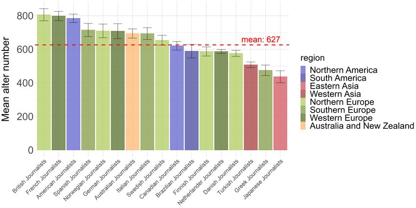
tend to engage with other journalists of similar popularity, and vice versa.
Journalist egos also tend to keep their popular colleagues in the more in-
timate layers, hence allocating more cognitive resources for them. Instead,
when interacting with generic users, journalists seem to value popularity only
for their innermost layers, but still much less than when they interact with
other journalists.
Keywords: online social networks, ego networks, Twitter, journalists

1. Introduction
     Online Social Networks (OSNs) have been shaping and transforming our
daily lives for more than a decade. Currently, there are 4.14 billion active
social media users and 4.08 billion active mobile social media users1 . With
easy access to the Internet, especially via mobile devices, we started to carry
our new communication mediums and online social groups everywhere we go.
We can thus participate in online communities more than ever, amplifying
the phenomenon known as cyber-physical convergence, whereby our offline
and online lives become tightly intertwined. The huge volume of information
produced online across different OSN platforms gives researchers new op-
portunities to analyze human behavior on large-scale data, overcoming the
limitations of survey-based traditional approaches. However, there is a two-
way exchange between our offline and online social life. On the one hand, we
are transferring and engaging with our offline relationships on online plat-
forms. On the other hand, we are establishing new relationships, which may
not have been even possible in the offline world (due, e.g., to long distances
and different time zones). Thus, not only academic studies on human behav-
ior in the offline world via OSN data but also the comparison between offline
and online human behavior have gained popularity. Within this latter line
of research, scientists have tried to understand if and to which extent our
offline and online relationships are similar. Their findings showed that the
structure of online relationships by and large mirrors that of offline ones [1].
     OSNs not only have shaped how we communicate socially with each other
but they have also redefined what is expected from professionals in terms
of online presence, especially for jobs that have a wide audience, such as
politicians, artists, and journalists. As for the latter, social platforms have

  1
      https://www.statista.com/statistics/617136/digital-population-worldwide/

                                            2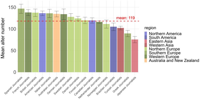
become digital newsstands, where user can find news sources and get instant
access to articles. Journalism has been under transition to keep up with this
new communication medium. Twitter has become one of the main access
points to news resources. According to a survey carried out by the American
Press Institute in collaboration with Twitter2 , 86% of Twitter users engage
with the platform for news. As a result, Twitter has become extremely
popular among journalists to share the news articles they produce, which
makes journalists an interesting professional group to analyze.
    According to the related literature, journalists use Twitter as a platform
for establishing their personal brands [2] and promote content from their
news websites [3]. Journalists are now individual brands, news and opinion
hubs [4], sometimes even more popular than the media companies they work
for. There are many studies analyzing this transformation of the profession [3,
4, 5], as well as several comparative studies on journalism. In [6], journalists
from the UK and 10 other European countries are compared in terms of their
role perception and their belief in the usefulness of the Internet. Another
study [7] analyzes Latin American journalists’ view on their professional role
in today’s digital media platforms and how they are organized to create a
new way of content management. In [8], cross-cultural research has been
carried out to assess the development of journalism culture in 66 countries.

                 Figure 1: Layered structure of human ego networks

   The above studies are mainly carried out via traditional survey-based
data collection and aim to understand journalism culture and journalists’
views on the transformation of the profession. In this work, we set out to
investigate the nature and structure of the relationships journalists entertain
on Twitter directly by studying their interactions on the platform. To this

  2
   https://www.americanpressinstitute.org/publications/reports/survey-research/how-
people-use-twitter-news

                                         3
aim, we leverage a graph-based abstraction known as ego network. The
latter describes the relationships between an individual (ego) and its peers
(alters) [9, 10, 11, 12]. Grouping these relationships by their strength, a
layered structure emerges in the ego network (Figure 1), with the inner circles
containing the socially closest peers and the outer circles the more distant
relationships. This structure originates from the limited cognitive resources
that humans are able to allocate to meaningful socialization (i.e., beyond
the mere level of acquaintances), as discussed in detail in Section 2. In this
model, five layers exist within the limit of the Dunbar number, which is the
maximum number of social relationships (around 150) that an individual,
on average, can actively maintain [12, 13]. Beyond the Dunbar number,
relationships are just acquaintances and their maintenance has a negligible
effect on the cognitive resources of the ego. The ego network is an important
abstraction, as it is known that many traits of social behavior (resource
sharing, collaboration, diffusion of information) are chiefly determined by its
structural properties [14]. To the best of our knowledge, there are no studies
on how journalists use their cognitive resources to maintain their relationships
on Twitter, and no comparative analyses of ego network-based behavioral
characteristics. In this paper, we study journalists from different countries
and continents in order to highlight similarities and invariants in their social
behavior online, and to understand how journalists allocate their cognitive
resources among their colleagues and non-colleague alters. Specifically we
address the following research questions:

RQ#1: How do journalists, as members of a specific community, organize
   their ego networks?

RQ#2 Does their geographical region affect how journalists organize their
   ego networks?

RQ#3 How do the ego networks of journalists change over time?

RQ#4 Are journalists topic-driven while establishing their relationships?

RQ#5 Does popularity play a role in how journalists engage with other
   users?

   The key findings presented in this study are the following:

                                       4
• Journalists whose Twitter interactions mostly rely on replies (such as
  those from Finland, the Netherlands, and Denmark) have a below-
  average number of alters, thus suggesting a tendency to get involved
  with the same group of people. This might hint at the fact that replies
  are a more personal/intimate communication with respect to mention
  and retweets, hence they consume more cognitive resources on the ego
  side, who, in turn, is able to interact with fewer people. Vice versa,
  the journalists that interact via retweets and mentions tend to engage
  with an above-average number of distinct peers, suggesting the opposite
  effect.

• Journalists establish numerous relationships, much more than generic
  Twitter users. However, when we consider only those relationships that
  are active (i.e., require a minimum cognitive effort), the ego network
  size (119 alters, on average) becomes very close to the Dunbar’s num-
  ber of 150. The social circle hierarchy of journalists also mirrors that
  observed for online networks, with an optimal number of social circles
  around 5.

• From a dynamic perspective, journalists have stable short-term re-
  lationships that don’t change a lot over time. They tend to keep
  their most and least intimate relationships as they are, while replacing
  the averagely intimate relationships much more. In the longer term,
  though, ego networks can be pretty dynamic, especially in the inner-
  most circles. This is in contrast with the findings about generic Twit-
  ter users [15] and suggests that the ego networks of journalists, while
  structurally similar to that of generic users, may be affected by the
  information-driven nature of journalist engagement on the platform,
  thus yielding to much more variability in the composition of rings.

• Journalists are topic-driven users. They establish their relationships
  through hashtags. A relationship is hashtag-activated if the first con-
  tact of the relationship includes a hashtag. Journalists have more
  hashtag-activated relationships than politicians and generic Twitter
  users. In addition, they tend to utilize hashtags for hashtag-activated
  relationships more than for the relationships that are not activated by
  hashtags. The percentage of hashtag usage is higher in inner circles
  that include more intimate relationships.

                                  5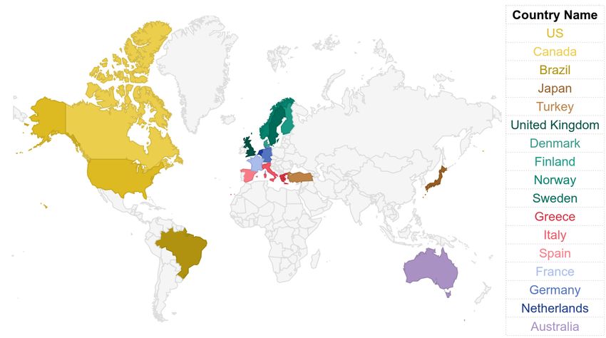
• Highly popular journalists tend to engage with other journalists of sim-
     ilar popularity, and vice versa, creating an assortativity in popularity.
     In addition, journalist egos tend to keep their popular colleagues in
     the more intimate layers, hence allocating more cognitive resources for
     them. Instead, when journalist egos interact with non-journalist alters,
     the alter popularity i) does not seem to play a role for relationships
     in the outermost circles, ii) has a smaller effect than for journalist-
     journalist relationships even in the innermost circles.
    The paper is organized as follows. In Section 2, we describe the Dunbar’s
ego network model and how we apply it. In Section 3, we describe how we
collected the datasets, how we cleaned and preprocessed them to determine
which journalists are suitable for ego network analysis. In Section 4, we show
the results of ego network analysis in four sub-sections with similarities and
differences between journalists from different regions in addition to compari-
son with politicians and generic Twitter users. In Section 5 we conclude the
paper. Given the large number of countries in our dataset, it will not be
always possible to provide plots for all of them. In these cases, the plots can
be found in the appendices.

2. The ego network model
    As discussed in Section 1, ego networks are graph-based abstractions used
to study the relationships between a tagged individual (called ego) and its
peers (alters). Specifically, an ego network is a local subgraph consisting
of the ego (in the center) and ties/links that connect the ego to its alters.
The strength of these links quantifies the emotional closeness/intimacy of
the ego-alter relationship, and it is commonly measured in the related liter-
ature through the contact frequency [12, 16, 17]. When the ego-alter ties are
grouped together [18, 1] based on their strength, intimacy layers emerge, as
shown in Figure 1. The typical sizes of each layer are 1.5, 5, 15, 50, 150,
respectively, where inner circles include alters with higher emotional close-
ness (higher contact frequency), and this closeness decreases through outer
circles. The size (150 alters) of the outermost circle is known as Dunbar’s
number. It represents the maximum number of relationships we can actively
maintain [12, 13]. An active relationship is defined as one having at least one
contact per year (see Sec. 2.1 for more details). The relationships beyond the
fifth circles are not active (just acquaintances), since we do not use our cog-
nitive resources regularly to maintain them. This finite-size layered structure

                                      6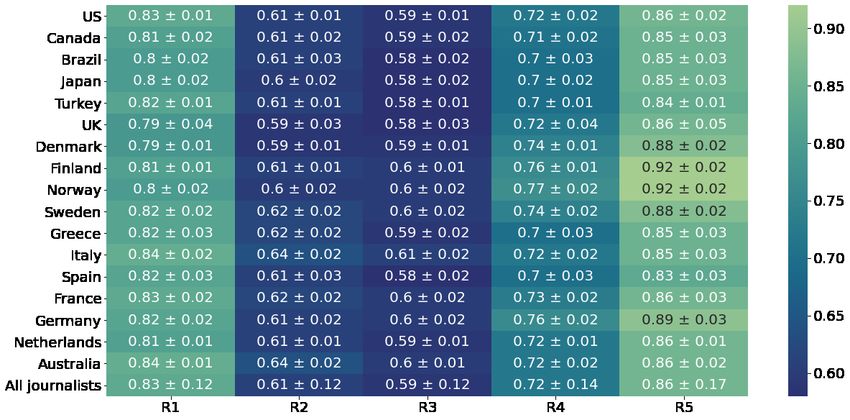
is the result of our limited information-processing capacity, and this finding
from anthropology goes under the name of social brain hypothesis [18]. Since
we have limited cognitive capacity and limited time, we try to optimize how
we allocate our cognitive resources among our relationships [14]. The result
of this optimisation is the ego network structure. An important structural
invariant of ego networks is their scaling ratio, defined as the ratio between
the sizes of consecutive layers. Its value is typically around three in the offline
and online networks studied in the related literature [1] [13].
    The existence of Dunbar’s ego network structures has been shown in dif-
ferent communication means in the offline world, including face-to-face inter-
actions [19], letters (Christmas cards) [12], phone calls [20]. Recently, their
occurence has been confirmed also for online interactions in OSNs [1, 21],
showing that the same cognitive capacity that limits our offline social inter-
actions exists also in OSNs (Facebook, Twitter). In this sense, OSN become
one of the outlets that is taking up the brain capacity of humans, and thus are
subject to the same limitations that have been measured for more traditional
social interactions, but are not capable of “breaking” the limits imposed by
cognitive constraints to our social capacity. Tie strengths and how they de-
termine ego network structures have been the subject of several additional
work. For example, in [22] authors provide one of the first evidences of the
existence of an ego network size comparable to the Dunbar’s number in Twit-
ter. The relationship between ego network structures and the role of users
in Twitter was analysed in [23]. In general, ego network structures are also
known to impact significantly on the way information spreads in OSN, and
the diversity of information that can be acquired by users [24]. In [21], the
ego network structure of politicians and how they allocate their cognitive
resources among the alters have been studied. In the study, they showed
the similarities between politicians’ ego networks and Dunbar’s model, and
differences between generic users’ ego networks by using Twitter data [1].
In addition to the characterization of the ego networks, the effect of ego
network structure on information diffusion has also been investigated in the
literature [25].

2.1. How to extract the ego network
    Dunbar’s ego network model captures how an individual allocates their
cognitive resources among their relationships. We do not allocate our cogni-
tive resources homogeneously across all the relationships that we establish.
Instead, we spend them mostly on the ones we try to keep “active” in our

                                        7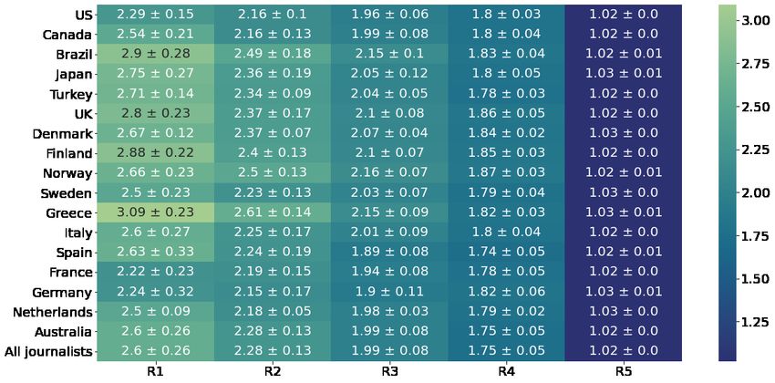
lives. In [12], an active relationship has been defined as one where at least
one contact per year occurs. This idea comes from the Christmas card ex-
change tradition of Western societies where people put effort to contact – at
least once a year – the people they value the most. In the related studies
about online ego networks [15, 1, 21], the concept of active relation has been
adapted to the online domain by calculating the frequency of direct contacts
and labelling as inactive those relationships with average contact frequency
smaller than one direct tweet per year (in analogy with the Christmas card
exchange in offline networks). In Twitter, a direct contact is a tweet (retweet,
reply, mention) where a user directly interacts with another user. Based on
direct contacts, we calculate the contact frequency for a relationship between
ego i and alter j as follows:
                              Nreply + Nmention + Nretweet
                      wij =                                ,                  (1)
                                         LR
where wij is contact frequency (which is a proxy for the intimacy between
the ego and the alter [12, 16, 17]), Nreply , Nmention , Nretweet are the total
number of replies, mentions, and retweets between the ego i and the alter
j, and LR is the observed duration (in years) of the relationship between i
and j, calculated as the time interval between their first direct tweet until
the download date of the dataset. In agreement with the related literature,
we filter out the relationships where LR is smaller than one year, since these
recently established relationships may not have yet stabilized [1, 26, 27].
    An active ego network of an individual consists of the relationships for
which the contact frequency (wij ) is bigger than one direct tweet per year. In
order to extract the intimacy layers as in Figure 1, these relationships must
be clustered into groups. Each layer includes relationships that have similar
intimacy with the ego. The number of layers, and the alters located in each
of them, can be determined by means of clustering algorithms. Similarly
to [28], in this work we use the Mean Shift algorithm [29], which is able
to automatically identify the optimal number of clusters without additional
interventions (e.g., k-means requires using the silhouette score or the elbow
method to this purpose). Thus, for each ego in our datasets, starting from the
active ego network, we derive the optimal number (typically around 5 in the
related literature) of intimacy layers and the alters assigned to them. Then,
we can easily compute the ego network scaling ratios as the ratio between
the sizes of consecutive layers (recall that this is typically an invariant, whose
value is around three).

                                        8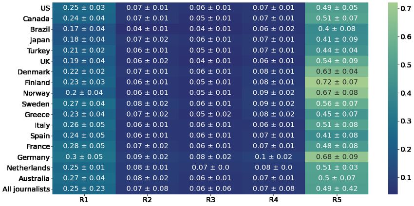
The ego networks obtained as described above are typically referred to as
static ego networks, and they will be studied in Section 4.1 for the journalists
in our datasets. By modelling the ego-alter ties through a static ego network,
we consider all the communications between the ego and the alter. This
analysis provides an essential starting point for understanding the ego-alter
interactions and for quantitative comparisons with other datasets studied in
the related literature. At the opposite end of the spectrum, the dynamic
analysis of ego networks focuses on their evolution over time. Specifically,
snapshots of one year are considered, each being shifted forward by a fixed
amount of time with respect to the previous one. For each snapshot we focus
on the alters that are members of each ring, where a ring is defined as the
portion of circle that excludes its inner circles. If we denote the set of alters
in consecutive circles i and i + 1 as Ci and Ci+1 , respectively, where ring Ri+1
is defined as Ci+1 − Ci . Conventionally, R1 is equivalent to C1 . Egos for
whom we observe less than two years of tweets are filtered out, as they are
not observed long enough to extract robust results. The dynamic analysis of
the journalists’ ego networks will be discussed in Section 4.2.
    With dynamic ego networks, the intimacy between the ego and alter may
decrease between two consecutive time intervals, resulting in the alter moving
from one circle to another one. In order to capture the stability of rings (in
terms of membership) over time, we use the Jaccard similarity, defined as the
ratio between the cardinality of the intersection and that of the union set of
the alters belonging to ring i in consecutive time intervals. We calculate the
Jaccard index Jaccardi of ring i as follows:
                                    T −1 (t)  (t+1)
                                  1 X Ri ∩ Ri
                       Jaccardi =                                            (2)
                                  T t=1 R(t)  (t+1)
                                         i ∪ Ri

where T denotes the total number of consecutive snapshots. The closer this
index to one, the higher the overlapping. In case of no overlap, the Jaccard
index is equal to zero. The amount of movements between rings is measured
through the Jump index, which simply counts (and then averages across all
alters in the ring) the number of jumps between rings. This index can be
computed as follows:
                                    T −1
                                  1 X X t,t+1
                          Jumpi =          ∆  ,                              (3)
                                  T t=1 j∈R j
                                              i

                                       9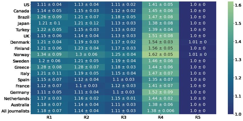
where we denote as ∆t,t+1
                       j    the number of jumps of alter j between snapshot
t and t + 1. For example, if the alter moves from R1 at t to R4 at t + 1, then
∆t,t+1
  j    will be equal to three. Of course, it is possible that, at t + 1, an alter
enters the active network from the outside. In this case, we assume that it
comes from the “last plus one” ring: e.g., for an ego with n social circles, the
alters is assumed to come from the (n + 1)-th ring.
    The notation we use in the paper is summarised in Table 1.

                    Table 1: Summary of notation (for a tagged ego)

   Name                         Notation    Definition/formula
   Active network                   A       ego-centered subgraph with weights
                                            greater than 1
   Optimal number of circles        τ       the results of the clustering on the edges
                                            in the active network A
   Social circle (or layer)        Ci       i-th social circles of the tagged ego, with
                                            i ∈ {1, . . . , τ }
                                              |Ci |
   Scaling ratio of layer i        ρi       |Ci−1 | , with i ∈ {2, . . . , τ }
   Ring                            Ri       Ci − Ci−1
                                             1
                                               PT −1 Ri(t) ∩R(t+1)
   Jaccard index of ring i      Jaccardi    T     t=1   (t)
                                                                i
                                                                (t+1)
                                                      Ri      ∪Ri
                                                PT −1 P
   Jump index of ring i          Jumpi      1
                                            T     t=1   j∈Ri        ∆t,t+1
                                                                     j

3. The dataset
    We downloaded the Twitter timelines of journalists belonging to 17 differ-
ent countries from 8 different continental regions. We classify geographical
regions (continents and continental regions) by using UN M49 (standard
country or area codes for statistical use3 ). The countries, which can be seen
in Figure 2, were selected based on the availability of journalists lists on
Twitter. Twitter lists are collections of Twitter accounts that are included
in a list by Twitter users with the aim of having a pool of accounts, generally
quite popular, that are related to a specific topic of interest. For our study,
we manually looked up lists including journalists from the same country4 .

  3
   https://unstats.un.org/unsd/methodology/m49/
  4
   The Twitter lists that we used as seeds can be found in https://github.com/
mustafatoprak/TwitterJournalistLists

                                           10
For some of the countries, we found more than one relevant list, and in this
case the lists are merged into one. Our dataset contains a different number
of journalists for each country, as it can be seen in Table 2 (under the before
filtering column). As a result of the Twitter API limitations, only the 3200
most recent tweets of each journalist (with a public profile) have been down-
loaded, and timelines without any tweeting activity were removed from the
dataset.
Figure 2: Countries in the dataset
3.1. Observability
Since the Twitter API only discloses the last 3200 tweets of any public
Twitter account, we were not able to download the full timelines of journal-
ists having more than 3200 tweets. We refer to these accounts as partially
observed, because we can only observe a portion of their timelines instead
of their full Twitter activity since their registration to the platform. Across
our datasets, on average 75.13% of the users are partially observed (i.e., they
posted more than 3200 tweets, see Table 2). We were able to fully observe
only 23.7% of the users (Table 2). Please note that being partially or fully
observed is an indirect measure of the user’s tweeting frequency: the more the
tweets posted, the quicker the 3200 slots are saturated. Indeed, the average
daily tweeting frequency, across all journalists datasets, is 0.5 tweets/day
for the fully observed users and 6.1 tweets/day for the partially observed
ones (note that this number is fully compatible with human activity). The
observability of the journalists’ timelines changes among the different coun-
tries: most of the datasets have at least 66% of the users that are partially
11Table 2: General statistics for the datasets
before filtering after filtering
fully observed(%) /
continent region dataset profiles (#) tweets (#) profiles (#) tweets (#)
partially observed(%)
Americas Northern America USA 1,722 4,671,922 617 1,927,183 10.86 / 89.14
Canada 917 2,462,998 427 1,281,149 20.14 / 79.86
South America Brazil 897 2,489,943 217 1,236,620 13.82 / 86.18
Asia Eastern Asia Japan 566 1,361,392 192 521,676 34.90 / 65.1
Western Asia Turkey 2,189 5,495,545 731 2,203,729 14.64 / 85.36
Europe Northern Europe UK 512 1,330,467 235 717,341 14.47 / 85.53
Denmark 3,694 3,725,084 656 1,671,441 50.00 / 50.0
Finland 936 1,477,304 321 824,823 46.11 / 53.89
Norway 1,190 1,504,906 201 584,251 28.86 / 71.14
Sweden 761 1,792,973 275 847,196 12.36 / 87.64
Southern Europe Greece 862 1,858,442 265 778,403 24.15 / 75.85
Italy 486 1,301,858 255 781,415 16.47 / 83.53
Spain 468 1,309,723 195 611,233 10.26 / 89.74
Western Europe France 559 1,525,600 323 975,941 21.98 / 78.02
Germany 405 879,071 146 415,560 30.14 / 69.86
Netherlands 4,303 9,621,422 1,674 4,859,433 27.18 / 72.82
Australia and
Oceania Australia 956 220,4974 400 1,153,010 29.50 / 70.5
New Zealand
1,260.18 2,647,860.24 419.41 1,224,831
All journalists mean ± sd ± ± ± ± 24.87 / 75.13
1,134.95 2,203,177.69 367.15 1,064,588
observed, except for the Danish and Finnish journalists where approximately
half of the users have partially observed timelines.
We define the observed timeline as the portion of the user’s timeline we
can access via the Twitter API. If the 3200-tweets API limitation is not hit,
the observed timeline is the same as the active timeline, which instead covers
the user activity starting from the date the user registered to Twitter until
the dataset was downloaded. Since the coverage of the timeline is based
on the number of tweets published by the user, the observed portion of the
timeline is user-based. As a result, if we measure the tweeting volume (total
amount of daily tweets over time) in the datasets, we observe a striking
growth in the most recent weeks (Figure 3a, gray curve). This is a spurious
effect, due to the fact that the observed timelines of the partially observed
users fall in the latter period of the dataset timeframe. This is evident when
plotting the number of active users who produced the corresponding tweeting
volume (blue curve in Figure 3a). As we can see from the figure, the plots
12(a) American journalists (b) Danish journalists
Figure 3: Tweeting volume and active users over time for two representative countries
start from the early days of Twitter5 (since we have fully observed users
whose observed timelines go back to the registration date). As we follow
the timelines throughout the later dates, we notice that, while the number
of active users increases (approximately linearly in most of the datasets),
the total tweet volume per day increases exponentially. While the behaviour
observed in Figure 3a well represents the general trend across several the
countries, there are also countries (like the Northern European ones, together
with Germany and the Netherlands) where the observed behavior is different.
As shown in Figure 3b for a representative country, very prolific journalists
do not seem to be part of the dataset in this case, and there is no exponential
growth of the tweeting volume in the most recent days of the datasets. The
plots for all the countries in our dataset can be found in Appendix A.1.
3.2. Keeping only real journalists
The Twitter lists that we used to identify our reference pool of jour-
nalists are created by other Twitter users. The general aim of these lists
is to provide a curated collection of news/information sources generally re-
lated to a specific country or region. Therefore, these lists may include not
only journalists but also news companies, anchormen, radio hosts, and so
on. Even though these accounts are sources of information, they are not
journalists. Including these accounts may lead us to a characterization of
ego networks that do not represent journalists accurately. Thus, we need to
apply a classifier to decrease the noise in the datasets. In order to correctly
identify “true” journalists, we have tested three different approaches (and
5
Twitter has been established in 2006.
13(a) British journalists (b) Italian journalists
Figure 4: MCC scores. In the plots, g represents the classifier that leverages the Google
Knowledge Graph, k represents the keyword extraction method, b represents the bot de-
tection classifier. The symbol & represents the logical AND operation, symbol | represents
the logical OR. They are used to specify the test combinations of the three classifiers.
their combinations). The first one is based on journalism-related keyword-
matching in the user Twitter bio (where the match involves words such as
columnist or correspondent). The second one entails searching for the per-
son’s job in the Google Knowledge Graph (GKG). The third one filters out
users that are marked as bots by the Botometer bot detector. For more
details, please refer to Appendix A.2. We have evaluated the performance
of these three classifiers – in isolation and combined – on a subset of jour-
nalists and non-journalists (Italian and English ones) that we have manually
labelled. Since the journalist/non-journalist classes are quite imbalanced in
our labelled dataset, we used MCC (Matthews’ Correlation Coefficient [30])
for assessing which combination performs best. The results are shown in Fig-
ure 4. The classifier jointly considering the information in the GKG together
with the keywords in the bio provides the best trade-off (high MCC, fewer
computational steps) on the labelled datasets. Thus, we used it for filtering
out non-journalists from the remaining datasets in our study. In the end, we
removed 7815 non-journalists.
3.3. Identifying the regular and active users
Of all the journalist users remaining after the filtering in Section 3.2, we
want to keep in our study only those that are regular and active Twitter
users. The inactive life of a user is defined as the time interval between the
last tweet of the user and the download time of the dataset. Long inactive
14periods are a sign of decreased engagement with the platform. In [15], a
user is accepted as inactive if there is no activity for the last 6 months
(mimicking Twitter 6-month inactivity criterion that labels users as inactive
if they do not login at least once every six month6 ). In this paper, we use
instead the intertweet time, which we have previously introduced in [27]. This
method assumes that a user has abandoned the platform if the inactive period
is longer than six months plus the longest period between two consecutive
tweets of the user. The intuition behind this formulation is to embed the
user’s personal regularity pattern (by considering their longest break in their
tweeting activity) instead of fixing an a-priori period of absence equal for all
users. Using this filter, 1169 users are marked as having abandoned Twitter
at the time we downloaded the dataset.
We now focus on how regular a user activity is. We assume that a Twitter
user is regular if, as in [21], the user posts at least one tweet every 3 days
as an average for at least half of the observed timeline. If this is not the
case, the user is labelled as sporadic. In Figure 5, we show the classification
of users both based on the abandonment classifier (previous paragraph) and
the regularity classifier. As expected, partially observed users are much more
active than fully observed one. For our analysis, we focus on regular and
active users, since they engage with the platform regularly and, thus, spend
on it more cognitive resources than others.
At the opposite end of the spectrum of inactive users are users that tweet
a lot. These users could have a significant impact on the ego network statis-
tics, due to their intense Twitter activity, hence should be studied separately.
In order to detect these outliers, we have run DBSCAN (a standard cluster-
ing technique that automatically identifies outliers [31]) on the journalists
tweeting frequencies. For all the datasets, we found that all the outliers fea-
ture an observed timeline shorter than one year (Appendix A.3). This is
due to the fact that, as these users produce numerous tweets per day, they
saturate the Twitter API limitation fast, hence their observed timelines are
too short. Given that their observed timelines are shorter than one year,
their ego networks are discarded, as discussed in Section 2.1.
The last check we perform is about the stationarity of the Twitter activity
of the users in our dataset. As previously shown in the literature ([25],
[20], [32]), newly registered social network users add relationships into their
6
https://help.twitter.com/en/rules-and-policies/inactive-twitter-accounts
15Figure 5: User classification
network and interact with others at a higher rate than long-term users. After
a while, their activity stabilizes. Newly registered users are thus outliers with
respect to the general population of users, and they should be discarded from
the analysis. Again, we use the approach described in [27]. We do not observe
a drastic change in tweeting activity for any of the datasets. Therefore, we do
not discard any part of the timeline as a transient period. For more details
on this analysis, please refer to Appendix A.4.
3.4. Dataset overview
The number of journalists in our dataset at the end of the preprocessing
phase is reported, per country, in Table 2. In Table 3 we provide some
summary statistics regarding the length of their active life on Twitter, their
average daily tweets, and their predominant type of tweet. With an average
Twitter life between 6 and 9 years, the journalists in out datasets tend to be
long-time Twitter users. These journalists tweet, on average, twice or thrice
per day. 65% of the tweets we observe are social tweets (reply, retweet 7 and
mention), i.e., entail a direct communication between two Twitter users.
When considering the split between the different flavours of social tweets
7
Quote tweets are treated as retweets.
16and indirect tweets, some trends emerge. Specifically, we can identify (Fig-
ure 6(b)) three distinct groups of countries. In the cluster denoted in blue in
Figure 6(b) (comprising Japan, Greece, Turkey, Brazil), the dominant tweet
type are indirect tweets. These journalists, thus, tend to post their tweets
without interacting with others, not even mentioning their news outlet. At
the opposite end of the spectrum, journalists in the red cluster predomi-
nantly engage on Twitter by means of replies. Interestingly, they all belong
to the same geographical area (Northern Europe). Note that replies are reac-
tive to what other people/news outlet have posted online. The third cluster
(members colored in pink) comprises all the English-speaking countries in
our dataset plus the Central and Southern European states. For these coun-
tries the prevalent mode of interaction is through retweets and mentions.
This is perhaps the most expected pattern of engangement for journalists on
Twitter: sharing content from other users and tagging users (among which,
their news outlets) in conversations. The clusters in Figure 6(b) are obtained
applying k-means clustering on their tweet type feature vector (shown in Fig-
ure 6(a)) that consists of elements that represent the percentage of tweeting
type (i.e., the tweeting type feature of Japanese journalists is [9, 7, 33, 52]
which corresponds to reply, mention, retweet, indirect tweeting types’ per-
centages). We select the number of clusters based on the silhouette method.
In Figure 6(b) we visualize these clusters by reducing the dimension of the
data to the first two PCA components to be able to represent the data in 2D.
Note that no geographical information has been used to obtain the clusters:
the fact that nearby countries tend to belong to the same cluster shows the
strong indirect effect of spatial correlation and similar cultures.
4. Ego network analysis
In this section, we analyze the ego network structure of the journalists
that have been filtered as described in Section 3, and we show the differences
and invariants between different countries and regions. The frequency of
direct tweets (mentions, reply, or retweets) is used to represent the strength
of the ties (that is, the intimacy or emotional closeness) between journalists
(egos) and their alters as discussed in Section 2.1. Recall also that, similarly
to the related literature, a relationship is considered active if the ego and the
alter have at least one contact (direct tweet) per year.
17(a) (b)
Japan 9 7 33 52 0.50 France
●
Turkey 14 11 33 41
●
Greece 15 11 27 47 Australia ● cluster 1
Canada 14 17 30 39
Italy 14 17 35 34 Italy
● ● cluster 2
France 15 19 38 28 retweet mention
0.25
Brazil 19 16 21 44 US ● cluster 3
●
Finland 25 10 28 38
PC2 (39.3%)
Spain
●
US 17 21 28 35
Germany
● ●
UK 23 15 30 33 Canada ●
Australia 17 21 33 28 UK
Spain 19 20 27 34
0.00 ●
Turkey
Germany 22 17 29 33
Netherlands 26 14 23 37
Norway 28 12 24 36 Finland Netherlands Sweden
● ●
Sweden 30 12 24 34 ●
●
●
● Japan ● Denmark
Denmark 32 11 24 32 −0.25 Greece ● Norway
Brazil reply
0% 25% 50% 75% 100%
indirect
−0.6 −0.3 0.0 0.3
indirect retweet mention reply
PC1 (52.14%)
Figure 6: Tweet types across countries. On the left, the average number of tweets in
the different categories, computed by country. On the right, the corresponding PCA
plot. The colors denote the 3 groups detected by the k-means clustering algorithm on the
PCA components. The optimal number of groups has been obtained using the silhouette
method.
4.1. Static properties of ego networks
The static view of an ego network is a single, aggregate snapshot of the
ego and its ties. It is a representation of the ego network that includes
the whole observed timeline of the journalist. This analysis allows us to
understand the general distribution of cognitive resources through all the
alters and to compare results with other findings from the related literature
in a quantitative manner (since the analysis of static ego networks is the
starting point in all related works).
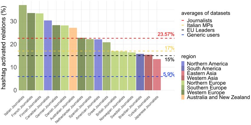
First, we show the average number of alters (with confidence intervals)
of egos in different countries (Figure 7, the distribution of the number of
alters per ego in each dataset, instead of dataset averages, can be found in
Figure A.6 of Appendix B). This number captures how many peers the ego
user interacts with during the last 3200 observed tweets, and it corresponds
to the size of the ego network when both active and inactive relationships
are considered (see Section 2). As expected, the countries whose journalists
engage on Twitter predominantly via indirect tweets (Figure 6(b)) tend to
feature fewer alters than their more social counterparts. Figure 7 also shows
that journalists that mostly rely on replies (such as those from Finland, the
18Table 3: Summary statistics
dataset statistic type active life [years] total tweets observed tweets tweet/day % social % replies % retweets % mention
US mean 9.08 13199.12 3123.47 3.24 65.41 25.27 43.30 31.42
sd 0.97 13407.07 318.19 2.02 16.89 19.56 22.28 19.60
Canada mean 8.04 10544.86 3000.35 3.30 61.35 23.45 49.47 27.08
sd 1.43 13027.79 511.59 2.19 19.47 19.26 22.49 18.92
Brazil mean 8.58 14874.91 3079.88 3.14 56.09 33.96 37.64 28.39
sd 1.59 16040.28 394.39 2.05 18.97 24.43 23.69 21.42
Japan mean 6.42 7416.97 2717.06 2.81 48.37 18.16 67.73 14.11
sd 2.33 7156.52 817.50 1.99 19.14 20.08 25.74 17.41
Turkey mean 7.49 11167.86 3014.68 2.94 58.67 24.57 56.25 19.17
sd 1.32 10180.01 465.07 1.80 19.73 20.45 24.22 16.550
UK mean 8.45 11369.24 3052.51 3.18 67.39 33.92 43.89 22.18
sd 1.07 10756.58 460.81 2.12 15.86 19.83 20.70 14.62
Denmark mean 7.14 5085.30 2547.93 2.01 67.63 47.02 36.04 16.93
sd 1.83 5795.11 822.68 1.59 14.80 24.10 22.11 13.57
Finland mean 6.36 5141.03 2569.54 2.28 62.18 39.51 44.65 15.84
sd 1.78 4791.04 840.97 1.77 16.93 22.59 22.34 13.93
Norway mean 8.59 6993.00 2906.72 1.78 64.29 43.98 36.78 19.24
sd 1.26 7303.59 586.30 1.21 17.66 22.74 22.44 15.63
Sweden mean 8.57 12047.46 3080.71 2.50 66.29 44.65 36.81 18.54
sd 1.08 12224.38 424.71 1.70 16.22 22.09 21.03 14.66
Greece mean 7.33 10426.07 2937.37 2.45 53.10 27.41 51.67 20.92
sd 1.29 15919.70 576.30 1.74 20.90 21.56 26.07 20.78
Italy mean 7.85 10536.59 3064.37 2.89 66.34 21.38 52.52 26.10
sd 1.30 8622.80 415.26 1.84 19.34 17.64 20.92 19.14
Spain mean 8.43 17051.02 3134.53 3.45 65.80 28.49 41.41 30.10
sd 1.07 14219.35 274.32 2.06 16.03 19.88 20.36 18.51
France mean 8.03 10269.97 3021.49 3.06 71.92 21.34 52.23 26.44
sd 1.30 9034.66 445.22 2.16 14.49 18.04 21.22 17.29
Germany mean 8.21 7810.44 2846.30 2.17 67.05 32.13 43.06 24.81
sd 1.32 7969.40 667.03 1.62 14.80 18.53 20.42 16.05
Netherlands mean 8.07 9889.23 2902.89 2.34 63.35 41.64 35.87 22.49
sd 1.52 12482.73 617.79 1.72 17.19 22.22 21.84 15.25
Australia mean 7.85 7146.85 2882.53 2.62 72.06 23.82 46.35 29.83
sd 1.43 5984.29 612.12 1.80 15.36 16.13 19.44 18.09
All journalists mean 9.08 13199.12 3123.47 3.24 65.41 25.27 43.30 31.42
sd 0.97 13396.81 317.94 2.02 16.88 19.54 22.26 19.59
Netherlands, and Denmark) have a below-average number of alters, thus
suggesting a tendency to get involved with smaller groups of people. This
is consistent with the fact that replies are a more personal/intimate com-
munication with respect to mention and retweets, hence they consume more
cognitive resources on the ego side, which, in turn, is able to interact with
fewer people. Vice versa, the journalists in countries from the pink cluster in
Figure 6(b) tend to interact with an above-average number of distinct peers,
hinting at the opposite effect. Even though there are differences for journal-
ists from different regions and countries, still the average number of alters of
journalists are much bigger than those of the generic Twitter users analyzed
in [1], where more than 90% of users have less than 100 relationships. This
19supports the claim that journalists establish more relationships and they are
prominent users on Twitter.
The number of alters showed in Figure 7 include relationships to which
egos don’t allocate their cognitive resources regularly (the typical case in the
anthropology literature, which we also apply here, is at least once a year). We
now consider the average number of active relationships of egos in different
countries (Figure 8, the distribution can be found in Figure A.7 of Appendix
B). As expected, the average number of active alters is significantly lower
than in the previous case of Figure 7, with sizes varying between 75 alters
(Japanese journalists) and 147 (Spanish journalists). Turkish, Greek and
Japanese journalists still have the smallest network sizes. Also, the differ-
ence between journalists and generic Twitter users still exists: the active
network size of generic Twitter users was 88 alters in [1], while the average
for journalists is 119. Hence, we can conclude that the ego network size
of journalists mimics offline ego network size predicted by Dunbar’s number,
and it is actually closer to the Dunbar’s number than those of generic Twitter
users were8 .
The active relationships of egos can be grouped into layers (also known
as Dunbar’s circles) based on their emotional closeness with the ego. It has
been shown that there are four layers in offline human ego networks [13]. This
number is extended to five layers for OSNs [1]. The optimal number of circles
can be determined by non-parametric clustering algorithms, as discussed in
Section 2. Figure 9 shows the distribution of the optimal circle number (i.e.,
the optimal number of relationship clusters, as found by Mean Shift) per ego
for all journalists (the distribution of circle numbers per dataset is provided
in Figure A.8 of Appendix B). The mode value of the optimal circle numbers
is 5, its mean value is 5.6, and its median value is 6. All datasets feature a
mean and median value for the optimal number of social circles around five,
thus matching the Dunbar’s model, with the exception of Japanese journalists
(which is not surprising given that their active ego network sizes are smaller
than for other countries). In the remaining of the paper, when comparing
8
While the initial filtering used in [1] is different from the one discussed in this paper
(Section 3), the comparison between the two sets of results is still meaningful. In fact,
the filtering in [1] (whereby only users with an average of more than 10 interactions per
month are kept) tends to retain only very active users, thus it might overestimate the
social interactions of generic users. However, our results indicate that journalists tend to
be even more engaged than this active subset of generic users.
20Figure 7: Average number of alters per ego, grouped by country
Figure 8: Average active networks size for egos in each country
Figure 9: Optimal number of circles per ego (red line: average, blue line: median)
21Table 4: Circle sizes of egos with optimal cicle number 5
dataset C1 ratio C2 ratio C3 ratio C4 ratio C5
US 3.24 ± 0.21 8.3 ± 0.51 20.15 ± 1.2 48.42 ± 2.52 124.56 ± 5.78
2.96 ± 0.21 2.58 ± 0.11 2.56 ± 0.08 2.72 ± 0.1
Canada 3.43 ± 0.27 8.29 ± 0.72 19.36 ± 1.68 44.68 ± 3.49 114.26 ± 7.53
2.63 ± 0.21 2.44 ± 0.12 2.46 ± 0.12 2.79 ± 0.18
Brazil 3.14 ± 0.31 8.19 ± 0.85 19.32 ± 1.93 43.27 ± 4.1 105.3 ± 9.43
2.98 ± 0.33 2.45 ± 0.12 2.32 ± 0.1 2.61 ± 0.17
Japan 2.98 ± 0.31 7.14 ± 0.65 16.4 ± 1.56 37.56 ± 3.77 96.2 ± 9.32
2.72 ± 0.3 2.35 ± 0.13 2.31 ± 0.1 2.67 ± 0.17
Turkey 3.1 ± 0.16 7.43 ± 0.43 17.46 ± 0.97 40.95 ± 2.05 106.54 ± 4.77
2.64 ± 0.15 2.46 ± 0.09 2.51 ± 0.07 2.79 ± 0.09
UK 3.5 ± 0.39 8.56 ± 0.94 22.08 ± 2.31 52.85 ± 4.71 134.07 ± 11.56
2.74 ± 0.32 2.72 ± 0.21 2.72 ± 0.32 2.66 ± 0.19
Denmark 3.63 ± 0.22 9.62 ± 0.58 22.69 ± 1.32 51.37 ± 2.9 119.87 ± 6.8
2.92 ± 0.17 2.5 ± 0.09 2.33 ± 0.06 2.41 ± 0.08
Finland 3.74 ± 0.37 9.29 ± 0.9 22.92 ± 2.11 53.57 ± 4.5 123.82 ± 10.05
2.74 ± 0.25 2.61 ± 0.17 2.49 ± 0.14 2.4 ± 0.1
Norway 3.35 ± 0.42 9.16 ± 1.09 21.74 ± 2.61 50.05 ± 5.29 115.56 ± 11.14
3.12 ± 0.35 2.47 ± 0.16 2.45 ± 0.13 2.42 ± 0.12
Sweden 3.38 ± 0.35 8.63 ± 0.86 20.86 ± 1.91 49.1 ± 3.97 122.77 ± 9.94
2.93 ± 0.27 2.61 ± 0.17 2.49 ± 0.13 2.6 ± 0.14
Greece 2.92 ± 0.28 6.66 ± 0.69 15.07 ± 1.68 34.5 ± 3.36 91.78 ± 7.68
2.49 ± 0.23 2.34 ± 0.16 2.44 ± 0.14 2.83 ± 0.16
Italy 2.81 ± 0.29 7.26 ± 0.79 19.2 ± 2.23 46.72 ± 4.81 124.21 ± 10.06
2.97 ± 0.37 2.73 ± 0.19 2.65 ± 0.18 2.94 ± 0.23
Spain 3.2 ± 0.3 8.34 ± 0.96 19.65 ± 2.39 46.97 ± 5.02 124.64 ± 10.65
2.74 ± 0.27 2.42 ± 0.16 2.59 ± 0.16 2.88 ± 0.2
France 3.2 ± 0.32 8.17 ± 1.06 19.46 ± 2.09 49.56 ± 4.56 129.14 ± 10.29
2.73 ± 0.26 2.65 ± 0.22 2.7 ± 0.13 2.78 ± 0.17
Germany 3.39 ± 0.54 8.99 ± 1.35 22.8 ± 2.97 52.99 ± 6.21 127.25 ± 13.74
3.1 ± 0.41 2.74 ± 0.23 2.45 ± 0.16 2.52 ± 0.23
Netherlands 3.28 ± 0.12 8.39 ± 0.31 19.9 ± 0.7 46.66 ± 1.53 114.79 ± 3.64
2.88 ± 0.11 2.49 ± 0.06 2.45 ± 0.05 2.55 ± 0.05
Australia 3.19 ± 0.29 8.06 ± 0.75 20.23 ± 1.84 49.17 ± 3.83 128.7 ± 8.67
2.82 ± 0.23 2.63 ± 0.15 2.63 ± 0.15 2.86 ± 0.19
All journalists 3.24 ± 0.05 8.3 ± 0.12 20.15 ± 0.28 48.42 ± 0.59 124.56 ± 1.35
2.96 ± 0.05 2.58 ± 0.03 2.56 ± 0.02 2.72 ± 0.02
egos with each other, we will focus on egos with five circles, in order to rule
out differences that are dependent on the different number of circles.
Table 4 shows the circle sizes (number of alters in each Dunbar’s circle).
As we can see from the last row of the table (corresponding to the average
of all journalists), the circle sizes of journalists are very close to the sizes
predicted by the Dunbar’s model (1.5, 5, 15, 50, and 150), with slight vari-
ations. Although generally the circle sizes of OSN users tend to be smaller
than what Dunbar’s model suggests [1, 21], journalists are an exception to
this rule, with more alters than expected in all circles except for the outer-
most one (5th circle). In Table 4, we also show the scaling ratio between
consecutive circles, whose typical value in the related literature is around
three [13]. Again, journalists conforms quite accurately to the predictions of
Dunbar’s model.
22Wrapping up the results of the static ego networks analysis, we can pro-
vide answers to the first two research questions laid out in Section 1.
RQ#1. Overall, journalists’ cognitive resource allocation to their alters mim-
ics closely what was observed in offline human ego networks, with the circle
sizes and the scaling ratio between the circle sizes matching Dunbar’s model.
Also, we have shown that journalists tend to have more active relationships
than generic Twitter users and politicians, with ego network sizes closer to
Dunbar’s number than typical OSN users.
RQ#2. The country in which journalists are active have an effect on their
ego network, but it does not alter significantly their structure. For example,
we have observed that Turkish, Greek and Japanese journalists have smaller
ego networks compared to other countries. British, French, and American
journalists engage in more numerous relationships on Twitter, while Span-
ish journalists maintain more active relationships. However, by and large,
Dunbar’s model holds across countries.
4.2. Dynamic properties of ego networks
In this section, we analyze the evolution of ego networks over time, in
order to capture changes in social relationships. If we divide the observed
timeline of a user into equal time intervals, the intimacy of a relationship
may change from interval to interval. That is, an ego may allocate more
cognitive resources to an alter in the early time intervals and less in the latter
ones, or vice versa. A varying intimacy entails a possible rearrangement of
relationships in circles. In order to investigate both short-term and long-term
dynamics, in this section we divide the observed timeline of an ego in one-
year time intervals with with 1-month step size (11 months overlap between
two consecutive time windows) and 12-month step size (no overlap between
consecutive time windows). Each time window provides a snapshot of the
ego networks, and, for each snapshot, we focus on rings (the portion of circles
excluding the inner circles) and how they change over time.
As discussed in Section 2.1, we study the dynamic changes in ego networks
by means of the Jaccard similarity and the Jump index. Considering the same
circle in two consecutive time intervals as two separate sets, the Jaccard index
is obtained dividing the cardinality of the intersection set by the cardinality
of the union set. The closer this index to one, the more the overlapping. The
amount of movements between rings is measured through the Jump index,
23which simply counts (and then averages across all alters in the ring) the
number of ring jumps made by the alters that have just entered the ring
at this temporal snapshot. Let us start our analysis with the short-term
changes of dynamic ego networks. Figures 10 and 11 show the values of
Jaccard and jump indices with 1-year time interval and 1-month step size
for the five rings. With this approach, we compare how ego networks change
on a month-by-month basis. The same analysis was carried out in [21] for
politicians. We can see (Figure 10) that the Jaccard indices are higher at
the innermost (R1) and the outermost (R5) rings, while middle rings have
lower index values (U-shaped pattern). This shows that the innermost and
outermost rings don’t change much over time, implying that the strongest and
weakest active relations of journalists are pretty stable in the short terms.
Vice versa, relationships with intermediate intimacy are more fluctuating.
These results are extremely consistent across countries. We provide Jump
index in Figure 11. The Jump indices are generally close to one and stable
across the rings, signalling that movements mostly occur between adjacent
rings. The ring with slightly more jumps, on average, is the fourth. This
may suggest that the fourth ring serves as a buffer zone, where mutating
relationships transit during their movements from one ring to another one.
Let us now study the long-term dynamics of ego networks. To this aim,
we consider 1-year time intervals for observing ego networks, and 1-year step
sizes (i.e., there is no intersection between two consecutive observation time
intervals). Results are shown in Figures 12 and 13. The U-shape pattern
across rings for the Jaccard coefficient is still there, but the similarity val-
ues are much lower. This means that, on a yearly basis, the rings of ego
networks tend to change significantly. In the central rings, especially, the
turnover is almost complete, as indicated by the Jaccard index close to zero.
Surprisingly, the most stable ring is R5, which contains the weakest active
social links. We observe slightly more variability across countries with re-
spect to the short-term results in Figure 10. This suggests that, as expected,
long-term dynamics tend to be more interesting than short-term ones. The
pattern observed for the Jump index, too, is completely different from the
previous case (Figure 11): the index decreases as we move from R1 to R5,
while previously it was stable across the rings and close to value of one. We
see that alters come to the first ring after moving from non-adjacent circles,
but this effect wanes as we move towards the outermost circles.
The results from this section allow us to provide an answer to the third
research question we laid out in Section 1.
24Figure 10: Jaccard coefficients of egos with optimal circle number 5 with 1-month step
size for 1-year intervals.
Figure 11: Jump indices of egos with optimal circle number 5 with 1-month step size for
1-year intervals.
25Figure 12: Jaccard coefficients of egos with optimal cicle number 5 with 1-year step size
for 1-year intervals.
Figure 13: Jump indices of egos with optimal cicle number 5 with 1-year step size for
1-year intervals.
26RQ #3. Journalists tend to have stable short-term relationships that don’t
change a lot over time. Specifically, they tend to keep unaltered their most
and least intimate relationships while they replace the relationships in middle
circles much more. In the longer term, though, ego networks can be pretty
dynamic, especially in the innermost circles. This is in contrast with the
findings about generic Twitter users [15] and suggests that the ego networks
of journalists, while structurally similar to that of generic users, may be
affected by the information-driven nature of journalist engagement on the
platform, thus yielding to much more variability in the composition of rings.
4.3. Social tweets and hashtags
Considering that journalists are on Twitter to promote their work, estab-
lish their personal brands, and satisfy the user demand for news, we expect
them to be more topic-driven than generic Twitter users. The typical way
of searching for and publishing tweets about a specific topic is to use hash-
tags. Thus, we expect journalists to be using hashtags at a higher rate than
regular users. To look into this aspect, we provide hashtag-related statistics
about the journalist datasets. Due to space constraints, we will provide plots
for selected countries (specifically, those representative of a group behavior),
while the complete set of results can be found in Appendix C.
In Figure 14, the percentage of hashtag-activated relationships are shown.
A relationship is labelled hashtag-activated if the first contact (direct tweet) of
the relationship includes a hashtag. For all journalists, the average hashtag-
activated relationship percentage is 23% while it is 6% for generic Twitter
users [1] and approximately 15% for politicians [21]. This confirms that
journalists establish more topic-driven relationships. All of the journalist
datasets have a higher hashtag-activated percentage than generic Twitter
users, and, in most cases, also higher than the politicians. However, when
we compare the different countries, there is a high variability in terms of
hashtag-activated relationship percentages, with values ranging from 12% in
Japanese journalists to 36% in Italian journalists.
Only showing the percentage of relationships activated by hashtags does
not give us information about the usage of hashtags across rings, i.e., about
the dependency on intimacy. In Figure 15, the percentage of hashtag-activated
relationships is shown for selected countries, in order to highlight three differ-
ent characteristics featured in the datasets. American journalists (together
with Finnish, French, and Netherlander ones, not shown in the figure) use
the same amount of hashtags across the rings. Hence, the percentage of their
27You can also read