Machine-learning scoring functions trained on complexes dissimilar to the test set already outperform classical counterparts on a blind benchmark ...
←
→
Page content transcription
If your browser does not render page correctly, please read the page content below
Briefings in Bioinformatics, 00(00), 2021, 1–21

                                                                                https://doi.org/10.1093/bib/bbab225
                                                                                Problem Solving Protocol

Machine-learning scoring functions trained on

                                                                                                                                                               Downloaded from https://academic.oup.com/bib/advance-article/doi/10.1093/bib/bbab225/6308682 by guest on 25 September 2021
complexes dissimilar to the test set already
outperform classical counterparts on a blind
benchmark
Hongjian Li , Gang Lu, Kam-Heung Sze, Xianwei Su, Wai-Yee Chan and
Kwong-Sak Leung
Corresponding author: Gang Lu, CUHK-SDU Joint Laboratory on Reproductive Genetics, School of Biomedical Sciences, Chinese University of Hong Kong,
Hong Kong. Tel: (852) 3943 5739; Fax: (852) 2603 5123; E-mail: lugang@cuhk.edu.hk

Abstract
The superior performance of machine-learning scoring functions for docking has caused a series of debates on whether it is
due to learning knowledge from training data that are similar in some sense to the test data. With a systematically revised
methodology and a blind benchmark realistically mimicking the process of prospective prediction of binding affinity, we
have evaluated three broadly used classical scoring functions and five machine-learning counterparts calibrated with both
random forest and extreme gradient boosting using both solo and hybrid features, showing for the first time that
machine-learning scoring functions trained exclusively on a proportion of as low as 8% complexes dissimilar to the test
set already outperform classical scoring functions, a percentage that is far lower than what has been recently reported on all
the three CASF benchmarks. The performance of machine-learning scoring functions is underestimated due to the absence
of similar samples in some artificially created training sets that discard the full spectrum of complexes to be found in a
prospective environment. Given the inevitability of any degree of similarity contained in a large dataset, the criteria for
scoring function selection depend on which one can make the best use of all available materials. Software code and data are
provided at https://github.com/cusdulab/MLSF for interested readers to rapidly rebuild the scoring functions and reproduce
our results, even to make extended analyses on their own benchmarks.

Key words: scoring function; machine learning; random forest; scoring power; binding affinity; blind benchmark

Hongjian Li received his PhD degree from Chinese University of Hong Kong in 2015. His research focuses on computer-aided drug design, scoring function
development, virtual screening and machine learning. He is the lead developer of the molecular docking software idock, the web server platform istar, the
WebGL visualizer iview and the scoring function RF-Score-v3. More information can be found at his website at https://github.com/HongjianLi.
Gang Lu is a senior research fellow in the School of Biomedical Sciences, Chinese University of Hong Kong. He established the bioinformatics unit and
currently engages in drug screening, drug repositioning, neural regenerative medicine, cell therapeutic strategies and disease diagnosis.
Kam-Heung Sze is an engineer in the Bioinformatics Unit, Hong Kong Medical Technology Institute. She works on computer-aided drug design, especially
data collection, software evaluation, script writing and computational pipeline automation.
Xianwei Su was an honorary research associate of the Chinese University of Hong Kong. His research interests lie in liquid biopsy, biomarker identification,
circulating miRNA, dendritic dell maturation and aneurysmal subarachnoid hemorrhage.
Wai-Yee Chan is the Director of the CUHK-SDU Joint Laboratory on Reproductive Genetics. He was the Director of the School of Biomedical Sciences and
the Pro Vice-Chancellor/Vice President of the Chinese University of Hong Kong. His expertise is in the molecular genetics of human reproductive and
endocrine disorders, biochemical genetics of inborn errors of copper and zinc metabolism, functional genomics and epigenomics.
Kwong-Sak Leung was a Chair Professor of Computer Science and Engineering in the Chinese University of Hong Kong. He is also a fellow of HKIE, a member
of IET and ACM, a senior member of IEEE and a chartered engineer. His research interests are in the areas of knowledge engineering, bioinformatics, soft
computing, genetic algorithms and programming, automatic knowledge acquisition, fuzzy logic applications and AI architecture.
Submitted: 3 March 2021; Received (in revised form): 27 April 2021
© The Author(s) 2021. Published by Oxford University Press.
This is an Open Access article distributed under the terms of the Creative Commons Attribution License (http://creativecommons.org/licenses/by/4.0/),
which permits unrestricted reuse, distribution, and reproduction in any medium, provided the original work is properly cited.
                                                                                                                                                      1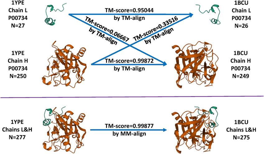
2     Li et al.

Introduction                                                           and X-Score, were basically insensitive [7]. Sze et al. proposed
                                                                       a revised definition of structural similarity between a pair of
In structural bioinformatics, the prediction of binding affinity
                                                                       training and test set proteins, introduced a different measure
of a small-molecule ligand to its intended protein is typically
                                                                       of binding pocket similarity, and benchmarked three classical
accomplished by a scoring function (SF). Before machine
                                                                       SFs and four RF-based SFs on CASF-2013. They found that even
learning (ML)-based SFs were invented, classical SFs relied on
                                                                       if the training set was split into two halves and the half with
linear regression of an expert-curated set of physiochemical
                                                                       proteins dissimilar to the test set was used for training, RF-
descriptors to the experimentally measured binding affinities.
                                                                       based SFs still produced a smaller prediction error than the best
ML-based SFs, however, bypass such prearranged functional
                                                                       classical SF, thus confirming that dissimilar training complexes
forms and deduce a, often immensely, nonlinear model from
                                                                       may be valuable when allied with appropriate ML approaches

                                                                                                                                              Downloaded from https://academic.oup.com/bib/advance-article/doi/10.1093/bib/bbab225/6308682 by guest on 25 September 2021
the data. Two comprehensive reviews have discussed the
                                                                       and informative descriptors [8].
outstanding performance of ML-based SFs over classical SFs
                                                                           Here we have expanded the above six studies from the fol-
in both scenarios of drug lead optimization [1] and virtual
                                                                       lowing perspectives. Firstly, we will demonstrate three exam-
screening [2]. Here we focus on the former scenario, particularly
                                                                       ples to show that the method employed by four early works
the problem of binding affinity prediction. To illustrate to what
                                                                       [3–6] for calculating structural similarity could be error prone,
extent the two types of SFs differ in predictive performance, we
                                                                       hence a revised method proposed lately [8] should be advo-
have compiled the results of 70 SFs and plotted Figure 1. It is now
                                                                       cated. Secondly, in addition to CASF-2016, a blind evaluation
obvious that ML-based SFs are taking an apparent lead ahead of
                                                                       was conducted too, where only data available until 2017 were
classical counterparts by a large margin.
                                                                       used to construct the SFs that predict the binding affinities
    One natural question to ask is whether the superiority of ML-
                                                                       of complexes released by 2018 as if these had not been mea-
based SFs originates from training on complexes similar to the
                                                                       sured hitherto [1]. This blind benchmark offers a complementary
test set. Exploring the influence of data similarity between the
                                                                       interpretation of the results. Thirdly, while building ML-based
training and test sets on the scoring power of SFs has resulted
                                                                       counterparts of classical SFs, exactly the same descriptors were
in a chain of studies recently (Supplementary Table S4). In 2017,
                                                                       preserved. In this way, any performance difference must neces-
Li and Yang measured the training-test set similarity in terms of
                                                                       sarily arise from the algorithmic substitution. The capability of
protein structures and sequences, and defined similarity cutoffs
                                                                       feature hybridization was assessed too. Finally, we discussed the
to construct nested training sets, with which they showed that
                                                                       limitations of CASF and the inevitability of similarity contained
random forest (RF)-based RF-Score lost to X-Score upon removal
                                                                       in a large dataset, giving advice on the criteria of SF selection in
of training complexes whose proteins are highly similar to the
                                                                       a prospective setting.
CASF-2007 test proteins identified by structure alignment and
sequence alignment [3]. However, in 2018 Li et al. found instead
that RF-Score-v3 outperformed X-Score when 68% of the most             Materials and methods
similar proteins were deleted from the training set, suggesting
that ML-based SFs owe a substantial portion of their perfor-           Figure 2 presents the overall workflow of this study, which will
mance to learning from complexes with dissimilar proteins to           be detailed in the following subsections.
those in the test set. Unlike X-Score, RF-Score-v3 was able to
keep learning with an increasing training set size, eventually
                                                                       Performance benchmarks
becoming significantly more predictive (Rp = 0.800) than X-Score
(Rp = 0.643) when the largest training set was used [4]. In addition   The CASF benchmarks have been broadly employed to assess
to quantifying training-test set similarity by comparing pro-          the scoring power of SFs. CASF-2016, the latest release, was
tein structures or sequences, in 2019 these authors presented          utilized as the test set, which offers the crystal structures and
a new type of similarity metric based on ligand fingerprints.          binding affinities of 285 complexes sampled from 57 clusters.
They observed that, regardless of which similarity metric was          After removing the test complexes from the PDBbind v2016
employed, training with a larger number of similar complexes           refined set, the rest 3772 complexes were used as the training
did not boost the performance of classical SFs such as X-Score,        set. This was the same configuration as used in [7].
Vina or Cyscore. On the other hand, XGB-Score, a SF utilizing              A recently proposed blind benchmark [1] mimicking the real-
extreme gradient boosting (XGBoost), was also shown to improve         istic process of structure-based lead optimization was adopted
performance with more training data like RF-Score-v3 [5]. In 2020      too, where the test set was constituted by 318 complexes from
Shen et al. further assessed 25 SFs, of which 21 are classical and     the PDBbind v2018 refined set not already included in the v2017
four are ML-based. Six ML methods, namely RF, extra trees (ET),        refined set. This test set is denoted Blind-2018 for short, on
gradient boosting decision tree (GBDT), XGBoost, support vector        which 2 classical SFs and 3 ML-based SFs had been evaluated
regression (SVR) and k-nearest neighbor (kNN), were employed           (Supplementary Table S5). It is totally different than CASF-2016
to build ML models using the features from the 25 SFs as well          since they do not overlap, i.e. not a single complex coexists
as their combinations. The results suggested that most ML-             in both test sets. The 4154 complexes in v2017 served as the
based SFs can learn not only from highly similar samples but           training set.
also from dissimilar samples with varying magnitude [6]. The               The scoring power of the considered SFs was measured by
above studies all used CASF-2007 as the sole benchmark. Su             three commonly used quantitative indicators, namely Pearson
et al. utilized CASF-2016 instead and calculated three similarity      correlation coefficient (Rp), Spearman correlation coefficient (Rs)
metrics considering protein sequence, ligand shape and binding         and root mean square error (RMSE). A better performance is
pocket. Six ML algorithms were evaluated, including Bayesian           signified by higher values in Rp and Rs and lower values in RMSE.
ridge regression (BRR), decision tree (DT), kNN, multilayer per-
ceptron (MLP), Linear SVR and RF. The RF model was found
                                                                       Similarity metrics
to possess the best learning capability and thus benefit most
from the similarity between the training set and the test set,         Obviously, the similarity of a training complex and a test
to which the three counterpart classical SFs, ChemScore, ASP           complex can be measured in multiple ways, for example by
Machine-learning scoring functions trained on complexes dissimilar to the test set                         3

                                                                                                                                                                             Downloaded from https://academic.oup.com/bib/advance-article/doi/10.1093/bib/bbab225/6308682 by guest on 25 September 2021
Figure 1. Performance of classical SFs (red dots) and ML-based SFs (green dots) on three CASF benchmarks. Each dot represents a SF. For instance, on CASF-2016
the best classical SF (i.e. X-Score) and the best ML-based SF (i.e. TopBP) obtained an Rp of 0.631 and 0.861, respectively. The raw values of this figure can be found in
Supplementary Tables S1–S3.

their proteins, their ligands or their binding pockets. The                            pockets was described by the city block distance between their
approach by Sze et al. [8] was employed to calculate the                               TopMap feature vectors encoding geometrical shape and atomic
similarity in terms of protein structure, ligand fingerprint and                       partial charges [13]. Note that the ligand fingerprint similarity
pocket topology.                                                                       also ranges from 0 to 1, but the Manhattan distance between
    In four early studies [3–6] the structural similarity between                      TopMap vectors ranges from 0 to +∞. Therefore, the latter
a pair of training and test set proteins was defined as the                            actually depicts the dissimilarity, rather than similarity, of the
TM-score [9] calculated from the structure alignment program                           two comparing pockets. A value of 0 suggests identity, and a
TM-align [10], which generates an optimized residue-to-residue                         larger value implies larger difference. Taken together, the three
alignment for comparing two protein chains whose sequences                             similarity metrics provide distinct but complementary ways to
can be different. Nonetheless, TM-align is restricted to aligning                      quantify the degree of resemblance of the training set to the
single-chain monomer protein structures. Given that nearly half                        test set.
proteins of the PDBbind refined set contain multiple chains,                               The pairwise similarity matrices can be found at the github
each chain was extracted and compared, and the lowest pair-                            repository. On CASF-2016 there are 285 complexes in the test set
wise TM-score was reported. This all-chains-against-all-chains                         and 3772 complexes in the training set, hence 285×3772 pairwise
approach could possibly step into the danger of misaligning a                          similarity values in the matrix. On Blind-2018 there are 318×4154
chain of a protein to an irrelevant chain in another protein. Three                    similarity values.
examples of misalignment are showcased in the Results section.
To circumvent such risk, we switched to MM-align [11], which
                                                                                       Training sets
is specifically developed for aligning multiple-chain protein–
protein complexes. It joins the multiple chains in a complex                           The original training set (OT) was split to a series of nested sets
in every possible order and aligns them using a heuristic iter-                        of training complexes with increasing degree of similarity to the
ation of a modified Needleman–Wunsch dynamic programming                               test set in the following way. At a specific cutoff, a complex is
algorithm with cross-chain alignments prohibited. Having been                          excluded from the original full training set if its similarity to
normalized by the test protein, the TM-score reported by MM-                           any of the test complexes is higher than the cutoff. In other
align was used to define the protein structure similarity. It falls                    words, a complex is included in the training set if its similarity
in the range of (0,1]. A TM-score close to 0 indicates the two                         to every test complex is always no greater than the cutoff [8].
comparing proteins are substantially dissimilar, and a TM-score                        Mathematically, for both protein structure and ligand fingerprint
of 1 implies identity.                                                                 similarities whose values are normalized to [0, 1], a series of
    Although the protein structure similarity considers the entire                     new training sets (NTs) were created by gradually removing
protein structure in a global nature, the binding of a small-                          complexes from the OT according to varying cut-off values given
molecule ligand to its intended macromolecular protein is                              a fixed test set (TS):
instead predominantly determined by the local environment
of the binding pocket. Locally similar ligand-binding domains
                                                                                                  NTsds (c) =       pi | pi ∈ OT and ∀qj ∈ TS, s pi , qj ≤ c           (1)
may be found in globally dissimilar proteins. For this sake,
it is rational to supplement extra measures to reflect ligand
similarity and pocket similarity. In terms of implementation,                          where c is the cutoff; pi and qj represent the ith and jth com-
the similarity of the bound ligands of a pair of training and                          plexes from OT and TS, respectively; and s(pi , qj ) is the sim-
test complexes was defined as the Tanimoto coefficient of                              ilarity between pi and qj . By definition, NTsds (1) = OT. When
their ECFP4 fingerprints [12], whereas that of the binding                             the cutoff varies from 0 to 1, nested sets of training complexes
4 Li et al.
Downloaded from https://academic.oup.com/bib/advance-article/doi/10.1093/bib/bbab225/6308682 by guest on 25 September 2021
Figure 2. Workflow of training and test set similarity analysis.
with increasing degree of similarity to the test set were con- In the case of pocket topology, since the values indicate
structed. For instance, with Blind-2018 as the test set, the protein dissimilarity instead of similarity and they fall in the range of
structure similarity cutoff starts at 0.40 and ends at 1.00 with [0, +∞], a slightly different definition is required:
a step size of 0.01, thereby generating 61 nested training sets.
Figure 3 shows a Venn diagram characterizing the relationship
between the test set and the nested training sets. The test
NTdds (c) = pi | pi ∈ OT and ∀qj ∈ TS, d pi , qj ≥ c (2)
set does not overlap any of the constructed training sets, but
the latter overlap each other, e.g. setting the cutoff to 0.40,
0.41 and 0.42 results in three training sets NTsds (0.40), NTsds (0.41) where d(pi , qj ) is the dissimilarity between pi and qj . Likewise,
and NTsds (0.42) with 334, 408 and 475 complexes, respectively, NTdds (0) = OT and NTdds (+∞) = ∅. When the cutoff steadily
and the latter is a superset of the former, i.e. NTsds (0.40) ⊆ decreases from +∞ to 0, nested training sets with increasing
NTsds (0.41) ⊆ NTsds (0.42). When the cutoff reaches 1.00, all the degree of similarity to the test set were generated. The pocket
4154 training complexes will be included in NTsds (1.00). Like- topology dissimilarity cutoff starts at 10.0 and ends at 0.0 with a
wise, the ligand fingerprint similarity starts at 0.50 and ends step size of 0.2, thus generating 51 nested training sets.
at 1.00 with a step size of 0.01, thereby creating 51 nested Analogously, the opposite direction was also considered,
training sets. where nested sets of training complexes with increasing degreeMachine-learning scoring functions trained on complexes dissimilar to the test set 5
Downloaded from https://academic.oup.com/bib/advance-article/doi/10.1093/bib/bbab225/6308682 by guest on 25 September 2021
Figure 3. Venn diagram depicting the relationship between the test set and the nested training sets on Blind-2018. The numbers of training complexes 4154, 3526, 3267,
. . . , 475, 408 and 334 correspond to the protein structure similarity cutoff values 1.00, 0.99, 0.98, . . . , 0.42, 0.41 and 0.40, respectively.
of dissimilarity to the test set were built as follows: entropy. Vina is a quasi-MLR model where the weighted sum
of five empirical terms is normalized by a conformation-
independent ligand-only feature codenamed Nrot, which
NTssd (c) = pi | pi ∈ OT and ∃qj ∈ TS, s pi , qj > c (3)
implies the degree of conformational freedom of the ligand. To
imitate this specialty, the original weight for Nrot was adopted
NTdsd (c) = pi | pi ∈ OT and ∃qj ∈ TS, d pi , qj < c (4) without recalibration while building MLR::Vina. A side effect
The former applies to protein structure and ligand fingerprint is that its RMSE performance will become unreliable, from
similarities, and the latter applies to pocket topology dissimilar- which we will avoid drawing conclusions. The RF counterparts
ity. By definition, ∀c, NTdds (c) ∪ NTdsd (c) = OT, NTdds (c)∩NTdsd (c) = ∅. RF::Vina [18] and RF::Cyscore [19] were generated with the same
The corresponding number of training complexes given a cutoff set of six descriptors from Vina and four descriptors from
can be found at the github repository. Cyscore, respectively. Supplementary Table S6 summarizes the
molecular features. The full feature set for all the complexes can
be found at the github repository.
Scoring functions Additionally, the features from X-Score, Vina and Cyscore
Classical SFs undertaking multiple linear regression (MLR) were were combined and fed to RF and XGBoost, thereby producing
compared to their ML-based variants. X-Score [14] v1.3 was RF::XVC and XGB::XVC (taking the first letter of each SF). The
chosen to be a representative of classical SFs because on CASF- purpose was twofold: to explore by how much the mixed descrip-
2016 it resulted in the highest Rp performance among a panel tors would contribute to the predictive accuracy, and to compare
of 33 linear SFs (Figure 1), many of which are implemented in between RF and XGB which are both tree-based ML algorithms.
commercial software [15]. It also performed the best on CASF-
2013 and the second best on CASF-2007 among classical SFs. It is
a consensus of three parallel scores considering four intermolec- Results and discussion
ular descriptors: van der Waals interaction, hydrogen bonding,
Misalignment caused by the
hydrophobic effect and deformation penalty. These constituent
all-chains-against-all-chains approach
SFs simply differ in the calculation of hydrophobic effect. To
create MLR::Xscore, the three parallel SFs were independently We first show that the all-chains-against-all-chains method
trained with coefficients calibrated on the nested training sets, employed in four early works [3–6] could lead to misalignment.
and then averaged to produce a consensus score. To make an ML- For example, the 3E5A entry in the CASF-2016 test set describes
based counterpart, the same six features were reused but MLR a crystal structure of aurora kinase A (chain: A; sequence
was replaced by RF, thus creating RF::Xscore. length: 264) in complex with a small-molecule inhibitor and
Given that X-Score dated back in 2002, two recent SFs, the targeting protein for Xklp2 (chain: B; sequence length: 33);
AutoDock Vina [16] v1.1.2 and Cyscore [17] v2.0.3, were also the 3UOD in the training set describes another crystal structure
selected to represent classical SFs. Vina was selected because it of aurora kinase A (chain: A; sequence length: 266) in complex
is highly cited and widely used. Cyscore was selected because with another small-molecule inhibitor. A reasonable alignment
it yielded the highest Rp among 19 linear SFs on CASF-2007 should be aligning 3UOD chain A to 3E5A chain A because they
(Figure 1). Cyscore is a strict MLR model composed of four both describe the main target protein. Were the all-chains-
intermolecular features: hydrophobic free energy, van der Waals against-all-chains approach employed, every chain would be
interaction energy, hydrogen-bond energy and the ligand’s extracted and aligned, and the lowest pairwise TM-score would6 Li et al.
Downloaded from https://academic.oup.com/bib/advance-article/doi/10.1093/bib/bbab225/6308682 by guest on 25 September 2021
Figure 4. Comparison between TM-align and MM-align when structurally aligning the 3UOD entry in the training set and the 3E5A entry in the test set of CASF-2016.
be used. In this case (Figure 4), aligning 3UOD chain A to 3E5A entry 1GJ8 to the test set entry 1C5Z, where MM-align reported
chain A would produce a TM-score of 0.95392 (Supplementary 0.99419 but the all-chains-against-all-chains approach reported
Material S1) whereas aligning 3UOD chain A to 3E5A chain B 0.03351, equivalent to an underestimation of as much as 0.96068.
would produce a TM-score of 0.36819 (Supplementary Material Remind that structures with a TM-score higher than 0.5 assume
S2), and therefore the latter would be reported as the similarity generally the same fold [10]. Hence, such underestimation could
score between 3UOD and 3E5A, which apparently does not regard structures supposed to be of the same fold wrongly to be
make sense. In contrast, with MM-align, aligning 3UOD to of distinct folds.
3E5A resulted in a TM-score of 0.84974, which seems rational. Overall, such bias is not a frequent phenomenon. Among all
Looking at the output of MM-align (Supplementary Material the 1 075 020 (=285×3772) pairwise similarities of CASF-2016,
S3), one may find that 3UOD chain A was in fact aligned to the portion where the difference in TM-score computed by the
3E5A chain A as expected, without enforcing an alignment on two approaches lies within 0.1 is 83%. This percentage is 85% on
3UOD chain B to 3E5A chain A. Hence, the all-chains-against- Blind-2018 over its 318×4154 similarities. When the difference
all-chains approach underestimates the similarity by 0.48155 threshold is relaxed to 0.2, the percentage increases to 95% for
in this example. Although one can still use TM-align to align CASF-2016 and 98% for Blind-2018, indicating a high degree of
proteins after manually joining the chains, this would lead to agreement by the two approaches in most cases, and thus the
suboptimal outcome with unphysical cross-chain alignments, conclusions in the four early studies employing TM-align are
which are prohibited in MM-align. unlikely to deviate much. Despite the consistency, we advocate
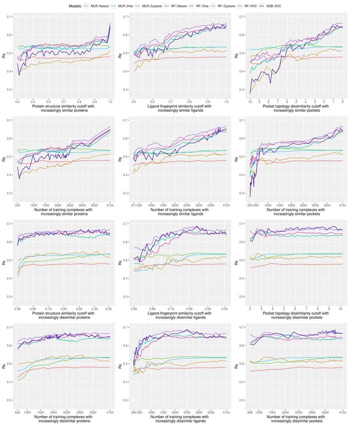
Another example is about aligning the 1YPE entry in the the more robust approach by MM-align, first introduced by Sze
training set to the 1BCU entry in the test set of CASF-2016 et al. [8].
(Figure 5). Both entries comprise two chains of thrombin, but
of different lengths. The L chain contains 27 and 26 residues
for 1YPE and 1BCU, respectively, whereas the H chain contains
250 and 249 residues. Were the all-chains-against-all-chains Skewed distribution of training complexes over
approach employed, four TM-score values would be generated (dis)similarity cutoffs
by TM-align and the lowest of them, 0.06667, would be reported We plotted the number of training complexes against the cut-
as the similarity score between 1YPE and 1BCU. This score, off values of the three similarity metrics where the test set
however, measures the degree of structural agreement between was CASF-2016 (Figure 6) or Blind-2018 (Figure 7), in order to
a thrombin light chain of 27 residues and a thrombin heavy chain show that training complexes are far from being evenly dis-
of 249 residues. As a result, it turns out to be understandably tributed. In reality, the distribution of training complexes under
low. In contrast, MM-align reported a TM-score of 0.99877, which the protein structure similarity metric is skewed, e.g. 628 training
seems reasonable because all the four chains describe the crystal complexes have a test set similarity greater than 0.99 (Figure 7,
structure of thrombin with the same UniProt ID. Hence, the top left subfigure). The rightmost bar alone already accounts for
approach by TM-align underestimates the similarity by 0.9321 15% of the OT of 4154 complexes. Incrementing the cutoff by
in this case. An analogous example is aligning the training set only 0.01 from 0.99 to 1.00 will include 15% additional trainingMachine-learning scoring functions trained on complexes dissimilar to the test set 7
Downloaded from https://academic.oup.com/bib/advance-article/doi/10.1093/bib/bbab225/6308682 by guest on 25 September 2021
Figure 5. Comparison between TM-align and MM-align when structurally aligning the 1YPE entry in the training set and the 1BCU entry in the test set of CASF-2016.
complexes. On the contrary, just 1.6% additional training com- by NTdds in Equation 2, and the sd direction specified by NTssd in
plexes will be included when the cutoff is incremented by the Equation 3 or by NTdsd in Equation 4.
same step size from 0.95 to 0.96. Hence, it is not surprising to
observe a substantial performance boost from raising the cutoff
Sharp leap in scoring power of ML-based SFs benefiting
by merely 0.01 if it is already at 0.99. This is more apparent in
the CASF-2016 benchmark (Figure 6, left column), where for as
from sufficient number of similar complexes for
many as 1033 training complexes (accounting for 27% of the training
full 3772 complexes) their test set similarities fall in the range Looking at the top left subfigure of Figure 9, which plots Rp
of (0.99, 1]. Thus one would reasonably anticipate a sharp leap performance on Blind-2018 versus protein structure similarity
in Rp performance of ML-based SFs in this particular range, cutoff, not unexpectedly sharp leaps are observed within the
as seen in previous studies [3, 8] and this study (see the next rightmost range of (0.99, 1] for all the five ML-based SFs. For
subsection). instance, the Rp notably increased by 0.067 (i.e. from 0.579 to
Such skewness can also be spotted, though less apparent, 0.646) for RF::Xscore, by 0.065 for RF::Vina, by 0.051 for RF::XVC,
in the distribution under ligand fingerprint similarity (Figures 6 as well as by 0.056 for XGB::XVC. This is also true on CASF-
and 7, center column), where 6.5% and 6.4% training complexes 2016 (Figure 8, top left subfigure; Figure 14, bottom two rows).
have a test set similarity greater than 0.99 under the CASF- Likewise, sharp leaps in Rs (Figures 10 and 11) and sharp drops
2016 and Blind-2018 benchmarks, respectively. The distribution in RMSE (Figures 12 and 13) are observed for ML-based SFs too
against pocket topology dissimilarity (Figure 7, right column), (e.g. the RMSE of RF::Xscore decreased by 0.11 from 1.45 to 1.34
nevertheless, seems relatively uniform, with just 0.1% com- on Blind-2018, versus a reduction of 0.05 in RMSE of the same SF
plexes falling in the range of [0, 0.2) and just 6% in the range within the second rightmost range of (0.98, 0.99] and a reduction
of [10, +∞). This pocket topology dissimilarity metric therefore of just 0.01 within the fourth rightmost range of (0.96, 0.97])
constitutes a useful tool to explore the impact of data similarity because, as explained in the subsection above, this particular
on the scoring power of SFs with training set size not so skewed range comprises as many as 27% and 15% training complexes
toward both ends of cutoff. of the CASF-2016 and Blind-2018 benchmarks, respectively, sug-
Bearing in mind the non-even distributions described above, gesting that ML-based SFs are effective at learning from training
we retrained the three classical SFs (MLR::Xscore, MLR::Vina and complexes highly similar to the test set.
MLR::Cyscore) and the five ML-based SFs (RF::Xscore, RF::Vina, Under the ligand fingerprint similarity metric (Figures 8–13,
RF::Cyscore, RF::XVC and XGB::XVC) on the nested training sets top center subfigure), such Rp and Rs performance leaps and
generated with protein structure similarity, ligand fingerprint RMSE drops for ML-based SFs within the rightmost range can
similarity and pocket topology dissimilarity, and plotted their be spotted too (e.g. the Rp of RF::XVC increased by 0.011 from
scoring performance on CASF-2016 (Figures 8, 10 and 12) and 0.657 to 0.668 and its RMSE decreased by 0.02 from 1.34 to 1.32
Blind-2018 (Figures 9, 11 and 13) in a consistent scale against on Blind-2018), though not as sharp because the distribution of
either cutoff or number of training complexes in two similarity training complexes is not as skewed (Figures 6 and 7, center
directions, i.e. the ds direction specified by NTsds in Equation 1 or column). Under the pocket topology dissimilarity metric8 Li et al.
Downloaded from https://academic.oup.com/bib/advance-article/doi/10.1093/bib/bbab225/6308682 by guest on 25 September 2021
Figure 6. Number of training complexes (the red curve) against protein structure similarity cutoff (left column), ligand fingerprint similarity cutoff (center column)
and pocket topology dissimilarity cutoff (right column) to the CASF-2016 test set in two directions, either starting from a small training set comprising complexes most
dissimilar to the test set (top row; the ds direction defined by NTsds or NTdds ) or starting from a small training set comprising complexes most similar to the test set
(bottom row; the sd direction defined by NTssd or NTdsd ). At the top row, the histograms plot the number of additional complexes that will be added to a larger set when
the protein structure similarity cutoff is incremented by a step size of 0.01 (left), when the ligand fingerprint similarity cutoff is incremented by 0.01 (center), or when
the pocket topology dissimilarity cutoff is decremented by 0.2 (right). At the bottom row, the histograms plot the number of additional complexes that will be added
to a larger set when the protein structure similarity cutoff is decremented by a step size of 0.01 (left), when the ligand fingerprint similarity cutoff is decremented by
0.01 (center), or when the pocket topology dissimilarity cutoff is incremented by 0.2 (right). Hence the number of training complexes referenced by an arbitrary point
of the red curve is equal to the cumulative summation over the heights of all the bars of and before the corresponding cutoff. By definition, the histograms of the
three subfigures at the bottom row are identical to the histograms at the top row after being mirrored along the median cutoff, but the cumulative curves are certainly
different. The raw values of this figure are available at https://github.com/cusdulab/MLSF.
(Figures 8–13, top right subfigure) where the distribution is capability and kept lifting performance persistently with more
relatively uniform (Figures 6 and 7, right column), no leaps training data (Figures 9, 11 and 13, top row), which was not
in Rp and Rs or drops in RMSE are visually detectable (e.g. seen in classical SFs. Although RF::Cyscore performed far worse
the difference in Rp of RF::XVC is less than 0.001 and the than MLR::Cyscore initially (e.g. Rp = 0.402 versus 0.444 and
difference in RMSE is less than 0.01 on Blind-2018, thus RMSE = 1.61 versus 1.57 at a cutoff of 0.4 under protein structure
not perceivably observable). These findings confirm that the similarity), through learning it kept improving and surpassed
remarkable performance gain obtained by ML-based SFs within MLR::Cyscore in Rp at a cutoff of 0.79 and in RMSE at a cutoff of
this range of cutoff is not exclusively due to the high similarity, 0.88. Their performance gap was widened when the full training
but also attributed to the considerable increase of training set was exploited, on which RF::Cyscore managed to yield a
set size. sharp leap, leading to much better performance (Rp = 0.513
versus 0.448, Rs = 0.515 versus 0.479, RMSE = 1.53 versus 1.59).
Thanks to the learning capability, even this least predictive
Learning capability of ML-based SFs as an advantage ML-based SF could improve Rp by 0.111 and reduce RMSE by
over classical SFs 0.08. Moreover, low-quality structural and interaction data,
All the five ML-based SFs exhibited learning capability to referring to those samples in the PDBbind general set but not
some extent, proliferating performance with larger sets of in the refined set, were previously found to improve the scoring
increasingly similar training samples. RF::XVC, empowered by its power of RF-based SFs [20]. Compounded with this beneficial
combination of features from three SFs, performed better than effect contributed by low-quality samples, the performance gap
their individual RF-based SFs on Blind-2018 (Figure 9), CASF- between RF-based and classical SFs is likely to be amplified.
2016 (Figure 8) and CASF-2013 [8]. The runner up was RF::Vina, In contrast, classical SFs lack such learning capability and
followed by RF::Xscore and lastly by RF::Cyscore, which somehow thus their performance curves nearly stay flat (Figure 9, top
underperformed on Blind-2018, CASF-2013 [8] and CASF-2007 row), as also seen recently [3–8]. For example, at the two ends
[6]. Despite being the least predictive among the group of four of protein structure similarity cutoff (i.e. 0.4 and 1.0), the Rp
RF-based SFs, RF::Cyscore still preserved the inherent learning varied slightly from 0.486 to 0.492 for MLR::Xscore, from 0.513Machine-learning scoring functions trained on complexes dissimilar to the test set 9
Downloaded from https://academic.oup.com/bib/advance-article/doi/10.1093/bib/bbab225/6308682 by guest on 25 September 2021
Figure 7. Same as Figure 2 but substituting the Blind-2018 test set.
to 0.519 for MLR::Vina, and from 0.444 to 0.448 for MLR::Cyscore. Low proportion of dissimilar training complexes
Surprisingly, unlike minor improvements were observed in Rp, required by ML-based SFs to outperform classical SFs
their RMSE even worsened a little bit, from 1.53 to 1.56 for
Evaluated in Rp on CASF-2016 (Figure 8, top left subfigure),
MLR::Xscore and from 1.57 to 1.59 for MLR::Cyscore (Figure 13,
RF::Xscore was not able to surpass MLR::Xscore, the best
top row). In Shen et al.’s study, the performance of Cyscore,
performing classical SF among the three, until the protein
ASP@GOLD, Alpha-HB@MOE and GBVIWSA-dG@MOE did not
structure similarity cutoff reached 0.99. The same is true on
change much with increasing similarity either [6]. In Su et al.’s
CASF-2013 [8] as well as on CASF-2007 where RF-Score was
study, ChemScore, ASP and X-Score were found to be basically
unable to outperform X-Score until the cutoff reached 0.98
insensitive to the similarity between the training set and the test
[3]. Hence it is not surprising for Li and Yang to assert that
set or the sample size of the training set [7]. This category of SFs,
ML-based SFs did not outperform classical SFs after removal
owing to insufficient model complexity with few parameters
of training complexes highly similar to the test set. However,
and imposition of a fixed functional form, could not benefit
this assertion does not hold when considering the RMSE metric
from more training data, even those that are most relevant
where RF::Xscore produced lower values than MLR::Xscore
to the test set, confirming again that classical SFs are unable
from a cutoff of 0.89 onwards (Figure 14, top row). Nor does it
to exploit large volumes of structural and interaction data [5,
hold upon substituting ligand fingerprint similarity (or pocket
7]. This is, in our opinion, a critical disadvantage given the
topology dissimilarity) where RF::Xscore started to overtake
continuous growth of structural and interaction data in the
MLR::Xscore when the cutoff reached just 0.80 on CASF-2016
future, which will further magnify the performance gap between
(Figure 8, top center subfigure) and 0.86 on CASF-2013 [8].
ML-based and classical SFs (Figure 1). To our surprise, such
Nor does this assertion hold on Blind-2018 (Figure 9, top left
a disadvantage was mistakenly regarded as an advantage by
subfigure) either where the best performing classical SF turned
others who claimed that the performance of X-Score is relatively
out to be MLR::Vina instead, which was surpassed by its RF
stable no matter what training data are used to fit the weights
variant RF::Vina at a cutoff of just 0.48. Now it is clear that this
of its energy terms [3], and a classical SF may be more suitable
assertion is restrictive on three conditions: the Rp or Rs metric,
when the target is completely novel [6]. Indeed, the performance
protein similarity and CASF benchmarks have to be employed.
of classical SFs is insensitive to training set composition (or in
Violating any condition voids the assertation.
other terms, stable), but it does not imply a better performance
As proposed previously [4], an alternative approach is to
than ML-based SFs (we will soon see that the opposite is true in
investigate the performance of SFs against the corresponding
most cases in the next subsection), and it is arduous to define
number of training complexes rather than the underlying cut-
‘completely novel’ given that a large training set may inevitably
off value. This approach had been adopted in subsequent stud-
contain any degree of similarity to the test set [4]. We will revisit
ies [5, 6, 8]. We therefore plotted the second row of Figure 9,
this argument after we discuss the limitations of the CASF
making explicit the number of complexes in each training set,
benchmarks later.
to evidence that ML-based SFs only required a small part of10 Li et al.
Downloaded from https://academic.oup.com/bib/advance-article/doi/10.1093/bib/bbab225/6308682 by guest on 25 September 2021
Figure 8. Rp performance of three classical SFs (MLR::Xscore, MLR::Vina and MLR::Cyscore) and five ML-based SFs (RF::Xscore, RF::Vina, RF::Cyscore, RF::XVC and
XGB::XVC) on the CASF-2016 benchmark when they were calibrated on nested training sets generated with protein structure similarity (left column), ligand fingerprint
similarity (center column) and pocket topology dissimilarity (right column). The first row plots the performance against cutoff, whereas the second row plots essentially
the same result but against the associated number of training complexes instead. Both rows present the result where the nested training sets were initially formed by
complexes most dissimilar to those in the test set and then gradually expanded to incorporate similar complexes as well (i.e. the ds direction). The bottom two rows
depict the performance in a reverse similarity direction where training complexes similar to those in the test set were exploited initially and then dissimilar complexes
were progressively included as well (i.e. the sd direction). The raw values of this figure are available at https://github.com/cusdulab/MLSF.
the full training set to outperform the classical SFs. MLR::Vina dissimilar to the test set under the protein structure similarity,
obtained the highest Rp among the three classical SFs con- ligand fingerprint similarity and pocket topology dissimilarity
sidered, yet it was outperformed by RF::Vina trained on 1159 metrics, respectively. Likewise, the second best performing clas-
(28% of the full training set), 271 (7%) and 617 (15%) complexes sical SF, MLR::Xscore, was outperformed by RF::Xscore trainedMachine-learning scoring functions trained on complexes dissimilar to the test set 11
Downloaded from https://academic.oup.com/bib/advance-article/doi/10.1093/bib/bbab225/6308682 by guest on 25 September 2021
Figure 9. Same as Figure 4 but substituting the Blind-2018 benchmark.
on 976 (23%), 271 (7%) and 504 (12%) complexes. These results three classical SFs, but it was overtaken by RF::Xscore trained
are remarkable in the sense that the two comparing SFs utilize on 1813 (44%), 292 (7%), 656 (16%) dissimilar complexes, and
the same set of features and differentiate each other by their by RF::XVC trained on 570 (14%), 271 (7%), 529 (13%) dissimilar
employed regression algorithm only. This trend is more obvious complexes (Figure 15). Taken together, these results reveal for
for RF::XVC. By integrating the features from X-Score, Vina and the first time that the proportion (i.e. 8%) of training complexes
Cyscore, it required just 703 (17%), 271 (7%) and 558 (13%) dis- dissimilar to the test set required by ML-based SFs to outperform
similar training complexes to surpass MLR::Vina, and 334 (8%), X-Score in Rp turns out to be far lower than what have been
271 (7%) and 529 (13%) to surpass MLR::Xscore. In terms of RMSE reported recently, i.e. 32% on CASF-2007 [5], 45% on CASF-2013
(Figure 13), MLR::Xscore obtained the lowest RMSE among the [8], and 63% on CASF-2016 (Figure 8).12 Li et al.
Downloaded from https://academic.oup.com/bib/advance-article/doi/10.1093/bib/bbab225/6308682 by guest on 25 September 2021
Figure 10. Same as Figure 4 but substituting Rs performance.
Recall that the TM-score magnitude relative to random struc- Greater contributions of similar training complexes
tures is not dependent on the protein’s size. Structures with than dissimilar ones
a score higher than 0.5 assume generally the same fold [10].
We now explore a different scenario, represented by the bot-
Coincidently, RF::Vina obtained higher Rp values than MLR::Vina
tom two rows of Figure 9, where the training set was originally
starting at a cutoff of 0.48. All the three classical SFs were
composed of complexes highly similar to those in the test set
overtaken by RF::XVC starting at a cutoff of 0.44 in terms of Rp
only and then regularly enlarged to include dissimilar com-
and 0.43 in terms of RMSE. Thus, the proteins of these training
plexes as well (i.e. the sd direction). The Rp curves of RF::Xscore,
samples do not assume the same fold, yet they contributed to
RF::Vina and RF::Cyscore are always above that of their respective
the superior performance of ML-based SFs.
classical SF, not even to mention their hybrid variants RF::XVCMachine-learning scoring functions trained on complexes dissimilar to the test set 13
Downloaded from https://academic.oup.com/bib/advance-article/doi/10.1093/bib/bbab225/6308682 by guest on 25 September 2021
Figure 11. Same as Figure 6 but substituting the Blind-2018 benchmark.
and XGB::XVC. Likewise, these ML-based SFs always generated investigated here. Consistently, most of the 28 ML-based SFs
lower RMSE values than their corresponding classical counter- benchmarked on CASF-2007 also showed a remarkably better
part (Figure 13) regardless of either the cutoff or the similarity performance than their corresponding classical ones [6].
metric. This is also true on CASF-2016 (Figure 12). These findings Consistent with common belief and hereby validated again,
constitute a strong conclusion that under no circumstances did training complexes similar to those in the test set contribute
any of the classical SFs outperform their ML variant. This was appreciably more to the scoring power of ML-based SFs than
one of the major conclusions by Li et al. on CASF-2007 [5] and dissimilar complexes. For example, RF::XVC yielded Rp = 0.654,
by Sze et al. on CASF-2013 [8], and now it is deemed generaliz- Rs = 0.623, RMSE = 1.40 when trained on 628 complexes (cut-
able to the larger CASF-2016 and Blind-2018 benchmarks being off = 0.99 in the sd direction) comprising proteins similar to14 Li et al.
Downloaded from https://academic.oup.com/bib/advance-article/doi/10.1093/bib/bbab225/6308682 by guest on 25 September 2021
Figure 12. Same as Figure 4 but substituting RMSE performance.
the test set (Figure 9, bottom left subfigure), versus Rp = 0.515, performance was achieved at a cutoff of 0.43 (corresponding
Rs = 0.511, RMSE = 1.50 when the same SF was trained on 703 to 3584 complexes) for RF::XVC, 0.53 (2629 complexes) for
complexes (cutoff = 0.84 in the ds direction) comprising dissimi- RF::Vina, and 0.88 (1651 complexes) for RF::Xscore. Such peaks
lar proteins (Figure 9, second row left subfigure). This result also were observed under all the three similarity metrics as well
rationalizes the sharp leap phenomenon observed in ML-based as on all the three CASF benchmarks [5, 8] (Figures 8, 10 and
SFs only. 12) and Blind-2018 (Figures 9, 11 and 13). Their occurrence is
Unlike in the ds direction where the peak performance likely owing to a compromise between the size of the training
for ML-based SFs was reached by exploiting the full training set and its relevance to the test data: encompassing additional
set of 4154 complexes, here in the sd direction the peak Rp complexes dissimilar to the test set beyond a certain thresholdMachine-learning scoring functions trained on complexes dissimilar to the test set 15
Downloaded from https://academic.oup.com/bib/advance-article/doi/10.1093/bib/bbab225/6308682 by guest on 25 September 2021
Figure 13. Same as Figure 8 but substituting the Blind-2018 benchmark.
of similarity cutoff would probably introduce noise. That said, the addition of more dissimilar proteins into the training set
the performance variation between ML-based SFs trained on a does not clearly influence the final performance too much
subset spawn from an optimal cutoff and those trained on the when there are enough training samples [6]. On the other hand,
full set is marginal. For instance, the Rp obtained by RF::XVC training ML-based SFs on the full set of complexes, despite being
trained on the full set was 0.668, just marginally lower than slightly less predictive than training on a prudently selected
its peak performance of 0.675 (for RMSE it was 1.32 with the subset, has the hidden advantage of a broader applicability
full set of 4154 complexes, also only marginally worse than domain, hinting that such models should predict better on more
the best performance of 1.30 obtained at a cutoff of 0.43 with diverse test sets containing protein families absent in the Blind-
3584 complexes), consistent with the recent conclusion that 2018 benchmark. Besides, this simple approach of employing16 Li et al.
Downloaded from https://academic.oup.com/bib/advance-article/doi/10.1093/bib/bbab225/6308682 by guest on 25 September 2021
Figure 14. Scatter plots of predicted and measured binding affinities on CASF-2016 (N = 285 test complexes). Three SFs are compared: MLR::Xscore (left column),
RF::Xscore (center column) and RF::XVC (right column), trained at three different cutoffs: 0.89 (1st row), 0.99 (2nd row) and 1.00 (3rd row), corresponding to 2179, 2739
and 3772 training complexes, respectively. The cutoff 0.89 represents the crossing point where RF::Xscore started to produce lower RMSE values than MLR::Xscore,
indicating that although ML-based SFs did not outperform classical SFs in terms of Rp after removal of training complexes highly similar to the test set, it is not true
when RMSE is considered. The cutoff 0.99 represents a training set without complexes highly similar to the test set (recall the skewed distribution in Figure 6), for
comparison to the cutoff 1.00 in order to demonstrate the sharp leap effect in Rp and Rs and the sharp drop effect in RMSE.
the full set for training does not bother to search for the optimal having distinct physiochemical semantics (such as geometric
cut-off value, which does not seem an easy task. Failing that features, physical force field energy terms and pharmacophore
would probably incur a suboptimal performance than simply features [21]), thus offering an opportunity to explore various
utilizing the full set. combinations and construct an optimal SF. RF::XVC was built
by combining features of X-Score, Vina and Cyscore, exhibiting
better performance than their individual RF-based SF. It obtained
Feature hybridizing capability of ML-based SFs as
an Rp of 0.668 on Blind-2018 (Figure 9), higher than that of
another advantage over classical SFs RF::Xscore (0.646), RF::Vina (0.649), and RF::Cyscore (0.513). Like-
Thanks to the nonlinear nature of ML models, it is not difficult wise, RF::XVC achieved an RMSE of 1.32 (Figure 13), lower than
to hybridize features from multiple existing SFs, even those that of RF::Xscore (1.34), RF::Vina (1.35) and RF::Cyscore (1.53). ItMachine-learning scoring functions trained on complexes dissimilar to the test set 17
Downloaded from https://academic.oup.com/bib/advance-article/doi/10.1093/bib/bbab225/6308682 by guest on 25 September 2021
Figure 15. Scatter plots of predicted and measured binding affinities on Blind-2018 (N = 318 test complexes). Three SFs are compared: MLR::Xscore (left column),
RF::Xscore (center column) and RF::XVC (right column), trained at three different cutoffs: 0.40 (1st row), 0.43 (2nd row) and 0.60 (3rd row), corresponding to 334, 570
and 1813 training complexes, respectively. The cutoff 0.40 represents the initial low end where MLR::Xscore resulted in a lower RMSE than RF::Xscore and RF::XVC. The
cutoff 0.43 is the crossing point where RF::XVC started to generate lower RMSE values than MLR::Xscore. The cutoff 0.60 is another crossing point where RF::Xscore
started to outperform MLR::Xscore in terms of RMSE.
also performed the best on CASF-2016 (Figures 8, 10 and 12) and and NNscore 2.0, which required 40% fewer training samples to
CASF-2013 [8]. Likewise, RF-Score-v3 [18] was built by hybridizing outperform classical SFs after hybridization. In the sd direction,
the original pairwise descriptors of RF-Score (i.e. occurrence in order to reach Rp ≥ 0.65, around 250, 300 and 250 training
count of intermolecular contacts between elemental atom type samples were compulsory for NNscore1.0, NNscore2.0 and RF-
pairs) with Vina empirical energy terms, which are two very Score-v2, respectively, whereas only 200 training samples were
different types of features. It was shown to perform better than mandatory for hybrid SFs [6]. In a comparative assessment of 12
RF-Score and RF::Vina on CASF-2007 [5]. RF-Score-v2 needed ML-based SFs on CASF-2013, 108 terms from RF-Score, BALL, X-
approximately 800 training samples to outperform classical SFs Score and SLIDE were used initially, which were subsequently
in the ds direction, but after hybridizing with GalaxyDock-BP2- reduced to just 17 terms with principal component analysis.
Score, Smina or X-Score, only around 550, 600 or 700 training Three resultant SFs, RF@ML, BRT@ML and kNN@ML, obtained
samples were needed [6]. More examples include NNscore 1.0 a Rp of 0.704, 0.694 and 0.672, respectively, higher than 0.61418 Li et al.
Downloaded from https://academic.oup.com/bib/advance-article/doi/10.1093/bib/bbab225/6308682 by guest on 25 September 2021
Figure 16. RMSE performance (left) and training time (right) of RF::XVC and XGB::XVC on the CASF-2016 benchmark when they were calibrated on different protein
structure similarity cutoffs.
achieved by the best of 20 classical SFs [22]. Although hybrid The excellent performance of RF over other ML algorithms
SFs do not necessarily outperform single ones, this available was also observed in two recent studies investigating the influ-
capability provides a chance to search for the best mixture of ence of data similarity. A comparative assessment of 25 com-
descriptors that would lead to peak performance. For instance, monly used SFs showed that GBDT and RF produced the best
hybridizing the pairwise descriptors of RF-Score into RF::XVC Rp values for most of the SFs on CASF-2007, performing bet-
could further reduce the required percentage (currently 8%) ter than ET, XGBoost, SVR and kNN [6]. Removing structurally
of dissimilar training complexes for ML-based SFs to surpass redundant samples from the training set at a threshold of 95%
classical SFs. on CASF-2016 effectively inhibited the learning capability of BRR,
In contrast, feature hybridization is tough for classical SFs DT, kNN, MLP and SVR except RF [7]. More examples include
which rely on linear regression. The energy term accounting RF@ML, which outperformed all other 11 ML algorithms on
for hydrogen bonding is present in X-Score, Vina and Cyscore, CASF-2013 [22].
but is implemented differently. How would one devise MLR::XVC Given that extensive efforts are usually compulsory for fine-
remains to be explored. Even more challenging is to merge tuning the hyperparameters of deep learning (DL) algorithms, it
two streams of features in distinct scales or units, such as is computationally prohibitive for us to conduct the systematic
merging the atom type pair occurrence count (without unit) trials presented here. There are evidences showing that DL-
used by RF-Score and the energy terms (in kcal/mol units) used based SFs were not always more predictive than those based on
by Vina. more established ML methods [1]. That said, it is worthwhile to
inspect deeper into this aspect in the future, since there are also
evidences showing that DL is competing RF in computational
Comparison between different ML regression methods docking [23].
Both RF and XGBoost are tree-based ML algorithms. Both RF::XVC
and XGB::XVC were demonstrated to possess learning capabil-
Limitations of the CASF benchmarks
ity and keep improving performance with training set size on
Blind-2018 (Figure 9) and CASF-2016 (Figure 8) in the ds direc- Six related studies [3–8] all employed the CASF benchmarks
tion, finally yielding a sharp leap. Here RF::XVC outperformed to investigate the impact of data similarity. These benchmarks
XGB::XVC under most settings, probably due to suboptimal tun- were formed by clustering a selected subset of complexes in
ing of the hyperparameters of XGB. As a reference, an XGB- the PDBbind refined set according to 90% similarity in protein
based SF utilizing the same set of descriptors as by RF-Score-v3 sequences, and only the clusters containing more than five
was found to marginally outperform the latter on CASF-2007 [5]. members (for CASF-2016) or three members (for CASF-2013 and
Regarding algorithmic efficiency, the training time required by CASF-2007) were considered. By construction, the CASF bench-
XGB::XVC was 19–50 times as much as that required by RF::XVC marks are affected by protein homology bias in that only pop-
(Figure 16). ular proteins having sufficient number of high-quality crystalMachine-learning scoring functions trained on complexes dissimilar to the test set 19
structures are included for benchmarking purpose, leaving out Inevitability of similarity contained in a large dataset
a large amount of unpopular proteins (e.g. only 285 test set
It was claimed that ML-based SFs are unlikely to give reliable pre-
complexes picked from 57 clusters of CASF-2016 versus 3772
dictions for completely novel targets [6], or may be less effective
training set complexes left in the refined set). By comparing
when dealing with structurally novel targets or ligand molecules
the results on CASF-2013, CASF-2016 and Blind-2018, it is clear
[7], but no formal definition for ‘novel’ was given. Here we come
that the CASF benchmarks overestimate the performance of
up with two possible definitions. The first is to set up a fixed
SFs, whether these are ML-based or not. For example, RF::XVC
similarity threshold, below which complexes are considered to
achieved Rp = 0.714, 0.754 and 0.668 on the three benchmarks,
be novel. Recall that at a protein structure cutoff of 0.40 (a
respectively. A decline of 0.086 in Rp ensued when transiting the
TM-score below 0.5 assumes generally distinct folds), which
benchmark from CASF-2016 to Blind-2018. Likewise, MLR::Xscore
corresponds to 334 (8%) training complexes, RF::XVC already
Downloaded from https://academic.oup.com/bib/advance-article/doi/10.1093/bib/bbab225/6308682 by guest on 25 September 2021
obtained Rp = 0.622, 0.647 and 0.492, respectively, equivalent to
generated a higher Rp than MLR::Xscore (Rp = 0.492 versus 0.486
a decline of 0.155, almost twice as much. Albeit the Rp perfor-
on Blind-2018). Hence the similarity threshold used to define
mance of both categories of SFs being overestimated by CASF,
novel has to be set to a rather low value in order for the two
some authors only saw the need of employing new benchmarks
claims to hold true. The second is to follow the old-fashioned
for ML-based SFs [7].
approach of leave-cluster-out cross-validation, where the whole
Although both categories of SFs suffered from performance dataset is first clustered by 90% sequence identity and then the
degradation on the more realistic Blind-2018 benchmark, the clusters are split to form nonoverlapping training and test sets
degree is different (Rp dropped by 0.155 for MLR::Xscore ver- [24]. The test complexes whose proteins do not fall in any of
sus just 0.086 for RF::XVC). This point can be revalidated from the training clusters are considered as novel. By leaving one
another perspective. The percentage of dissimilar training com- cluster out, an early study showed that the Rp averaged across
plexes required by RF::XVC to outperform X-Score was 45% on 26 clusters was 0.493 for MLR::Cyscore, 0.515 for RF::CyscoreVina
CASF-2013 and 63% on CASF-2016, far higher than just 8% on and 0.545 for RF::CyscoreVinaElem [19], indicating that ML-based
Blind-2018. This means X-Score performed unusually well on SFs hybridizing Cyscore features with those of Vina and RF-
CASF, making it tough for ML-based SFs to excel. In fact, X- Score still outperformed Cyscore itself, rendering the two claims
Score was the best performing classical SF on CASF-2016 and wrong. To make them right, one may further harden the chal-
CASF-2013 and the second best on CASF-2007 (Figure 1). Hence lenge by leaving two or three clusters out. No matter which defi-
the CASF benchmarks tend to overestimate the performance of nition, overoptimizing the training set composition to artificially
classical SFs much more than that of ML-based SFs. toughen the benchmark without considering the full spectrum
We think of two ways to circumvent the effect of overes- of complexes to be found in a prospective environment can
timation brought by CASF. The first is to employ the Blind- lead to false confidence. Adding training complexes that are
2018 benchmark [1], which is by construction a blind test in similar to the test set to some extent actually helps mimic a
that only structural and interaction data available until 2017 real scenario, as they represent the overall characteristics of the
are used to build the SF that predicts the binding affinities of existing available samples.
complexes released in 2018 as if these had not been measured Recently we asserted that a large dataset may inevitably
yet. Thus this benchmark realistically imitates a prospective contain proteins with any degree of similarity to those in the
scenario without introducing artificial factors that specifically test set [4]. Here we provide concrete statistics to support this
harden the challenge for either category of SFs. Another way is to assertion. A TM-score below 0.17 corresponds to randomly cho-
embrace the concept of soft overlap [7], with which training sets sen unrelated proteins [9], but neither any of the 3772 training
were compiled from the PDBbind refined set by removing redun- complexes nor any of the 4154 training complexes has a test
dant samples under four different similarity thresholds of 80%, set protein structure similarity below 0.17 on CASF-2016 and
85%, 90% and 95%. However, we think that these nonredundant Blind-2018, respectively, suggesting that the training and test
training sets are of little use because five of the six tested ML- proteins are unavoidably related. When relaxing the TM-score
based SFs all outperformed the three comparing classical SFs. filter to no higher than 0.5, only 1562 (out of 3772) and 1343 (out
The authors should instead provide a training set where ML- of 4154) training complexes can be assumed having different
based SFs fail to outperform classical ones, but such a training folds [10], still less than half of the full set. Even though one
set is understandably difficult to provide because when the sim- can find a training complex that is sufficiently dissimilar to the
ilarity threshold decreases, the sample size decreases too, down test set under all the three similarity metrics investigated in this
below a so-called ‘healthy’ size of around 2100 complexes, which study (or the 3-in-1 combined metric [7]), there may exist an
corresponds to the number of complexes of the nonredundant extra metric under which this particular training sample shows
set compiled from the smallest refined set (i.e. v2016) under the a high similarity. Therefore, it is inevitable for a large dataset
lowest threshold (i.e. 80%). This issue can be addressed either by to exhibit a certain degree of similarity to the test set. In this
discarding CASF-2016 as the test set, which these authors had context, it is meaningless to argue whether or not the training
not attempted, or by shrinking the sample size (or the similarity set contains samples similar to the test set, or whether overes-
threshold) to a point where the niche of classical SFs could timation occurs. What is really meaningful is whether the SFs
be appreciated [4]. Regarding the latter, remind that RF::XVC can make the best use of such similarity inherently contained
required merely 334, 271 and 529 dissimilar complexes to sur- in the training set. Nothing is wrong if one can make a reason-
pass MLR::Xscore under the three similarity metrics. Should able prediction based on the available information on similar
these nonredundant sets be useful for comparing ML-based and samples [7]. The statement that the performance of ML-based
classical SFs, their sample size probably has to be reduced to SFs is overestimated due to the presence of training complexes
below 271, which is about a half quarter of the healthy sample similar to the test set [6] can be alternatively interpreted as that
size they wanted to preserve. These sets, nevertheless, can be the performance of ML-based SFs is underestimated due to the
useful for examining the learning capability of ML-based SFs absence of similar samples in those artificially created training
with increasingly similar samples. sets that specifically harden the challenge for ML-based SFs.You can also read