Feasibility of fishery independent longline surveys for snapper, hāpuku, bass, and bluenose

Feasibility of fishery independent
longline surveys for snapper,
hāpuku, bass, and bluenose
New Zealand Fisheries Assessment Report 2020/25

 B. Hartill,
 V. McGregor,
 I. Doonan,
 R. Bian,
 S.J. Baird,
 C. Walsh

ISSN 1179-5352 (online)
ISBN 978-1-99-002596-9 (online)

August 2020

Requests for further copies should be directed to:

Publications Logistics Officer
Ministry for Primary Industries
PO Box 2526
WELLINGTON 6140

Email: brand@mpi.govt.nz
Telephone: 0800 00 83 33
Facsimile: 04-894 0300

This publication is also available on the Ministry for Primary Industries websites at:
http://www.mpi.govt.nz/news-and-resources/publications
http://fs.fish.govt.nz go to Document library/Research reports

© Crown Copyright – Fisheries New Zealand

TABLE OF CONTENTS

EXECUTIVE SUMMARY 1

1. INTRODUCTION 3

2. METHODS AND RESULTS 4
 2.1 Longline survey design for SNA 1 4
 2.2 Longline survey design for hāpuku/bass 9
 2.3 Longline survey design for bluenose 26

3. CONCLUSIONS AND RECOMMENDATIONS 38

4. ACKNOWLEDGMENTS 39

5. REFERENCES 40

APPENDIX 1: SNA 1 survey approach proposed by the 2016 SNA 1 Strategy Group 41

APPENDIX 2: Interviews with commercial SNA 1 bottom longline fishers 43

APPENDIX 3: Interviews with commercial hāpuku/bass bottom longline fishers 57

EXECUTIVE SUMMARY

Hartill, B.; McGregor, V.; Doonan, I.; Bian, R.; Baird, S.J.; Walsh, C. (2020). Feasibility
of fishery independent longline surveys for snapper, hāpuku, bass, and bluenose.

New Zealand Fisheries Assessment Report 2020/25. 64 p.

This report examines the potential feasibility of longline surveys designed to monitor trends in the
abundance of snapper in SNA 1, and nationally, for hāpuku/bass and bluenose. The analyses presented
in this report were based on commercial fishing events where these species were caught or targeted,
and the latitude and longitude of the start position was reported. Spatial survey strata were inferred from
spatial distributions of CPUE data, and improvements in survey estimate precision were evaluated given
the optimal allocation at different levels of sampling effort across these strata, based on the mean and
variance of catch rates reported in each stratum over a five year period between 2013–14 and 2017–18.

Survey strata could not be delineated from the spatial distribution of bottom longline snapper target
catch rate data for East Northland and Hauraki Gulf, or from the distributions of bottom longline and
bottom trawl data reported for the Bay of Plenty, given the high within cell variability seen within grid
cell CPUE data. Spatial survey strata were therefore based on stratum boundaries used for the most
recent snapper trawl surveys conducted in each region, resulting in six strata for East Northland and the
Bay of Plenty, and three for the Hauraki Gulf. All strata fall into one of three depth bands: 0 to 25 m,
> 25 to 50 m, and > 50 to 100 m. Optimal Neyman allocations of sampling effort across all strata within
each region, based on the mean and the variance of the catch rates reported in each stratum in any given
year, suggest that a target CV of 25% would be achieved if a standardised longline was deployed at
only three stations in each stratum. A recommendation from this work is that twice as many sites should
be surveyed in the first year, following a two-phase survey design, because analyses were based on
catch rate data provided by commercial fishers who would have targeted their effort towards areas of
higher expected abundance.

The spatial distribution of reported events targeting and or catching hāpuku/bass and bluenose was more
patchy, and boosted regression tree modelling was therefore used to assign grid cells to non-contiguous
spatial strata falling within the EEZ, based on event catch rates reported for each location, and digital
terrain model predictions for 23 environmental variables at each location. Four separate interpretations
of the available catch rate data were used to infer the abundance of hāpuku/bass, and separately for
bluenose, at each location. These abundance metrics were: the proportion of non-zero catch events and
the average of the logged non-zero catch rates at each location; when all of the available catch effort
were used, and when the analysis was restricted to those events where the only target species codes
reported were HPB, HAP, BAS, and BNS.

The stratum definitions that produced the most precise predictions of hāpuku/bass abundance were
those based on logged non-zero catch rate data for those events were only HPB, HAP, BAS, & BNS
were targeted. Simulations suggested that a 50 station longline survey based on these stratum definitions
would have achieved a target CV in four out of the five years assessed, but this level of precision was
not considered realistic for a national survey, because the abundance of hāpuku and of bass would also
differ by year and fish stock. The feasibility of a simplified three stratum survey for just the HPB 1
stock was therefore assessed, based on catch rates reported in each stratum for those events where all
species were targeted, and where only HPB, HAP, BAS, & BNS were targeted, and similar estimates
of survey precision were achieved. Discussions with a highly experienced commercial longline fisher
suggest, however, that even a single stock longline survey is unlikely to be cost-effective, because it
would usually be possible to deploy only a single longline per survey day. There are also concerns that
any survey based on features where fish are known to aggregate would provide a series of relative
biomass indices that were hypostable. An alternative catch-at-age sampling catch curve monitoring
approach is therefore proposed instead.

Fisheries New Zealand Feasibility of fishery independent longline survey designs • 1

The same analytical approach was also used to assess the viability of a national bluenose longline
survey, which also suggested that acceptably precise survey estimates could be obtained by a 50 station
survey, based on survey strata inferred from HPB, HAP, BAS, & BNS catch rate data. But a longline
survey is also not considered viable for bluenose, because this species also aggregates around structured
seafloor features and catch rates are also likely to be hyperstable. The cost of such a survey would also
be potentially prohibitive, because only one site could be surveyed per day.

2 • Feasibility of fishery independent longline survey designs Fisheries New Zealand

1. INTRODUCTION

Standardised CPUE indices are commonly used to monitor the status of many of New Zealand’s fish
stocks and are one of the primary analytical tools that underpin Fisheries New Zealand’s Harvest
Strategy Standard approach to fisheries management. Most of the CPUE indices that have been
developed for New Zealand fish stocks are based on generalised linear modelling (GLM)
standardisations of commercial catch effort data; but in some circumstances commercial fishers operate
in ways that can undermine the inherent assumption that catch rates are proportional to abundance
(Harley et al. 2001, Maunder et al. 2006). For example, commercial fishers may target habitats or
spawning aggregations where catch rates remain high, despite declines in abundances elsewhere. Catch
rate standardisations often fail to take account of improvements in fishing technology and practice, and
those changes are not apparent in the standard format catch effort returns that fishers are routinely
required to submit. Factors such as these can mask and underestimate the actual rate at which a fish
stock’s abundance may be changing, which is commonly termed “hyperstability”. The reliance on
commercial catch effort data may also be problematic when fishing effort does not occur throughout
the full spatial extent of a population’s range, either for economic reasons or because some areas may
be closed to one or more fishing method. Fishery independent data are therefore needed at times, to
provide a more robust measure of relative change in abundance.

Fishery independent longline surveys can be designed to overcome (and potentially assess) many of the
limitations of commercial CPUE standardisations, leading to greater certainty and confidence in
fisheries management. Fishery independent longline surveys have been used elsewhere to track changes
in fish abundance (Sigler 2000, Hanselman et al. 2015, Stewart et al. 2016), where intentionally
standardised longline fishing gear is deployed in a consistent manner according to a random stratified
design, in a conceptually similar manner to the research trawl surveys that Fisheries New Zealand
already commission to monitor high value fish stocks. The purpose of this study is to investigate the
feasibility of fishery independent standardised longline surveys, that could be used to monitor the
relative abundance of the snapper (Pagrus auratus) SNA 1 stock and for national surveys for
hāpuku/bass (Polyprion oxygeneios & P. americanus) and for bluenose (Hyperoglyphe antarctica).

The rationale for each of these surveys differs. The need for a fishery independent abundance survey
was identified as a research priority in the 2016 SNA 1 Management Plan (SNA 1 Strategy Group 2016;
as specified in Appendix 1), with longlining offering the most viable means of catching snapper across
all habitat types. With the hāpuku/bass fishery, Paul (2002) concluded that standardisations of
commercial drop line/longline CPUE data could not be used as an index of abundance, because most
of the catch was recorded as HPB and abundance trends may differ for these two species. Further,
although hāpuku/bass are managed as seven HPB fish stocks, Paul (2005) suggested that existing data
could not be used to describe the stock structure of New Zealand groper, because a reasonable degree
of movement was likely between areas. A fishery independent longline survey may therefore offer a
viable means of monitoring trends in abundance and the age composition across one or multiple HPB
stocks. A review of methods for the estimation of the relative abundance of bluenose in 2002 concluded
that the most promising survey method available was a fishery independent longline survey (Blackwell
& Gilbert 2003). Standardised commercial CPUE indices have been used to inform the most recent
bluenose stock assessment (Starr & Kendrick 2013), but there are concerns that changes in fisher
behaviour in response to cuts to catch limits cannot be modelled, undermining confidence in these
indices.

Designs for fishery independent longline surveys for SNA 1, hāpuku /bass, and bluenose are therefore
proposed here, based on modelling of catch effort data reported by commercial bottom longline fishers
catching these species during the 2013–14 (2014) to 2017–18 (2018) fishing years. The feasibility of
these designs is also assessed following interviews with commercial fishers, to determine whether a
standardised and spatially randomised longline survey could be used to monitor stock abundance and
composition in a reasonably consistent and unbiased fashion.

Fisheries New Zealand Feasibility of fishery independent longline survey designs • 3

Overall Research Objective

Determine the feasibility of fishery independent longline surveys for monitoring abundance and age
structure of inshore finfish

Specific Objectives:

 1. To design a bottom longline survey for snapper, Pagrus auratus, in SNA 1.

 2. To design a national bottom longline survey for hāpuku, Polyprion oxygeneios, and bass, P.
 americanus.

 3. To design a national bottom longline survey for bluenose, Hyperoglyphe Antarctica.

2. METHODS AND RESULTS

2.1 Longline survey design for SNA 1

A characterisation of the bottom longline snapper fishery in SNA 1 and subsequent analyses to inform
the design of a SNA 1 bottom longline survey were based on an extract of catch effort data from the
Fisheries New Zealand warehou database, for the five most recent fishing years; from 1 October 2013 to
30 September 2018. Catch and effort data were extracted for all bottom longline (BLL), bottom trawl (BT),
and precision bottom trawl (PRB) fishing trips, where snapper was either targeted during any event in
Statistical Areas 001 to 010 or landed from SNA 1 (rep log 12070). Trip numbers were used to link landed
catch weights to fishing events, so that the landed snapper catch weight could be prorated across fishing
events based on the estimated snapper weight reported for that event.

Catch effort data reported for two fishing methods were used to characterise the relative spatial
abundance of snapper and the likely variability of bottom longline catch rates within proposed survey
boundaries. These two methods were: bottom longlining, which occurs throughout East Northland and
almost all of the Hauraki Gulf (Statistical Areas 005, 006, and 007), but is only used in the western Bay
of Plenty (Statistical Areas 007, 008, and 009 for all of this region); and bottom trawling, which is often
used to target snapper in deeper waters than those fished by longliners and is the main fishing method
used to catch snapper in the eastern Bay of Plenty (Figure 1).

4 • Feasibility of fishery independent longline survey designs Fisheries New Zealand

a) Bottom longline

 b) Bottom trawl

Figure 1: Spatial distribution of the SNA 1 catch taken by bottom longlining (top panel) and bottom
 trawling (bottom panel) during the five year period from 2013–14 to 2017–18.

Bottom longlining and bottom trawling between 2013–14 and 2017–18 accounted for: 70 to 86% of the
snapper catch landed from East Northland (Statistical Areas 002 and 003), 50 to 75% of that landed
from the Hauraki Gulf (005, 006, and 007), and 50 to 75% of that landed from the Bay of Plenty
(Table 1). Latitude/longitude catch position data were available for between 3485 and 4389 bottom
longline events a year in SNA 1 during the five assessed fishing years, and 1683 to 3822 bottom trawl
events. The number of reported bottom trawl fishing events has declined in recent years, because some
bottom trawlers have started to carry both traditional otter trawl and precision bottom trawl fishing gear,
which they use interchangeably, depending on the area fished and market requirements. Precision
bottom trawl data were only used to prorate estimated catches reported during mixed bottom

Fisheries New Zealand Feasibility of fishery independent longline survey designs • 5

trawl/precision trawl event trips and were not used to inform the design of any of the proposed longline
surveys.

Table 1: Annual national tonnage of snapper landed from the SNA 1 fish stock by region, by fishing year
 and by fishing method.

 East Northland 2013–14 2014–15 2015–16 2016–17 2017–18

 Bottom longline 628 626 700 778 881
 Bottom trawl 337 320 357 319 165
 Precision bottom trawl – – 22 159 334
 Danish seine 188 170 136 161 104
 Set net 15 15 14 11 9
 Other 5 6 7 5 8
 Total 1 173 1 138 1 236 1 434 1 502

 Hauraki Gulf 2013–14 2014–15 2015–16 2016–17 2017–18

 Bottom longline 714 585 579 608 462
 Bottom trawl 548 585 416 279 72
 Precision bottom trawl – – 103 159 189
 Danish seine 367 496 406 338 315
 Set net 51 46 34 39 32
 Other 2 3 2 1 3
 Total 1 682 1 716 1 539 1 424 1 072

 Bay of Plenty 2013–14 2014–15 2015–16 2016–17 2017–18

 Bottom longline 375 434 412 434 404
 Bottom trawl 755 654 598 614 479
 Precision bottom trawl 0 0 89 208 501
 Danish seine 402 440 467 358 354
 Set net 4 4 2 3 6
 Other 5 13 3 38 15
 Total 1 542 1 545 1 572 1 655 1 759

The bottom longline survey designs for East Northland, the Hauraki Gulf, and the western Bay of Plenty
were based solely on standardised bottom longline catch rate (kg/hook) data. Commercial fishing effort
is targeted towards areas where the highest catch rates are expected, so any randomised sampling of
fishing events would be biased towards areas of high abundance. A gridbased prediction of the relative
abundance of snapper occurring seasonally throughout each region was therefore generated by
assigning fishing event catch rate data to 0.05 latitude/longitude degree squares, based on the reported
start position for each event. These catch rate data were then standardised by cell and fishing year to
describe the likely spatial distribution of snapper abundance and predict the catch rate expected at any
randomly located survey station, regardless of any spatial heterogeneity in the intensity of fishing effort.

Meaningful stratum boundaries for a SNA 1 bottom longline survey were not readily apparent from
spatial patterns seen in commercial longline catch rate data. Proposed survey strata were therefore based
instead on the strata used for the most recent snapper trawl survey in each region. Multiple trawl survey
strata were sometimes combined to produce larger bottom longline survey strata for three depth ranges:
0 to 25 m, > 25 to 50 m, > 50 to 100 m (Figure 2). The boundaries between strata adjacent to regional
boundaries coincided with Statistical Area boundaries, i.e., the boundary between 003 and 005 for the
East Northland/Hauraki Gulf boundary, and between 005 and 008 for the Hauraki Gulf/Bay of Plenty
boundary.

6 • Feasibility of fishery independent longline survey designs Fisheries New Zealand

Figure 2: Survey strata for bottom longline surveys for snapper for three regions of SNA 1: for East
 Northland (ENLD), the Hauraki Gulf (HAGU), and the Bay of Plenty (BPLE).

Although the spatial extent of the area fished by the commercial bottom longline fishery covers most
of the likely snapper habitat in SNA 1, very few longline events were reported in the eastern strata of
the Bay of Plenty (see Figure 1), and it was therefore necessary to use bottom trawl fishing event catch
rate data to infer the spatial density of snapper for these strata. Bottom trawling occurs throughout the
area defined by these three eastern strata, but almost no longlining is done east of Whakatane.

The measure of effort used to calculate bottom trawl catch rates (kg/hour towed) is not comparable with
that calculated from bottom longline events (kg/hook). A q was therefore calculated from the ratio of
these two method-specific catch rates, to scale trawl catch rates to a comparable level to longline catch
rates and provide a standardised measure of relative abundance across the Bay of Plenty, regardless of
which fishing methods fished in any location. These q ratios were calculated for each 0.05 latitude
degree cell in the Bay of Plenty where both methods had reported fishing events during a fishing year,
so that a global q could be calculated from the mean of catch rate ratios that had been standardised by
year and cell.

The number of stations required for a bottom longline survey in each region to achieve a target
coefficient of variation (CV) was initially determined by using the R package Allocate (Francis 2006).
These predictions of optimal sampling effort across strata were based on the mean and variance of
standardised longline (or for the eastern Bay of Plenty strata, longline scaled bottom trawl) catch rates
calculated for all 0.05 degree cells occurring within each survey stratum, with an initial minimum
allocation of three samples per stratum. These analyses suggested that a target CV of 25% would be
achieved for each regional survey if the minimum allocation of three longline sets was allocated to each
stratum (Table 1). Similar CV estimates were achieved when these allocations were based on catch rate
data reported during individual years, and for all years combined.

The reliability of these survey precision estimates was then assessed by generating 500 bootstrap survey
biomass estimates, to see if the CV of these estimates was similar to that predicted by Allocate, which
was based on summary statistics calculated from all of the available data. A sample of 500 bootstrap

Fisheries New Zealand Feasibility of fishery independent longline survey designs • 7

estimates was generated for each region, for each season (Summer – December to February; Winter –
June to August) during each of the five fishing years for which catch effort data were available. Three
survey station locations were selected at random from each stratum (given a 5 km minimum distance
exclusion zone between each station location) and the catch rates of the fishing event closest to each of
these station locations was used to calculate the biomass in each stratum, and across all strata, for each
bootstrap run. The CVs of the 500 bootstrap estimates of population abundance calculated for each
fishing year could then be compared with the survey estimate CVs predicted by Allocate, for each region
in each season. The CVs calculated from these bootstrap simulations were very similar, but slightly
higher than those given in Table 1.

Table 2: Predicted estimates of precision for seasonal bottom longline surveys conducted in three regions
 of SNA 1, where three survey stations were assigned to each stratum (see Figure 2).

 Region Season 2014 2015 2016 2017 2018 Minimum Maximum Mean Median

 East
 Northland Summer 13.8 16.3 16.7 19.0 0.15 0.15 19.0 13.2 16.3
 Winter 13.6 15.0 20.5 16.6 17.5 13.6 20.5 16.6 16.6

 Hauraki Gulf Summer 20.0 19.0 20.0 22.0 20.0 19.0 22.0 20.2 20.0
 Winter 20.4 19.9 24.6 20.7 21.6 19.9 24.6 21.4 20.7

 Bay of Plenty Summer 24.9 17.2 20.4 20.1 19.0 17.2 24.9 20.3 20.1
 Winter 13.8 15.6 16.9 20.4 18.1 13.8 20.4 17.0 16.9

All the survey biomass precision estimates predicted by Allocate and the bootstrap simulations were
within a target CV of 25%, which suggests that bottom longline surveys could be used to monitor
regional trends in snapper abundance. The ranges of the annual CVs calculated for all the scenarios
given in Table 2 are reassuringly tight. But it should be noted that these survey precision estimates were
based on commercial catch and effort data reported when targeting economically productive areas of
higher expected abundance, which will have varied by season. The CVs achieved by a fully random
and non-targeted snapper longline survey may therefore be higher than these predictions would suggest,
and more than three survey stations should be allocated to each stratum during the first survey year to
allow for this uncertainly. It would be prudent to adopt a two-phase survey design, with at least five
survey stations allocated to each stratum during the first phase of a survey, and a further 15% of the
overall effort allocated during the second phase, given the relative variability in catch rates observed in
each stratum during the first phase. The results of the first survey could then be used to inform the
design of subsequent surveys.

Any longline survey that is used to monitor snapper abundance should be based on standardised fishing
gear, to ensure comparability over time. The specification of a standardised gear configuration, however,
should be based on gear that is currently used by commercial fishers, because this gear would probably be
deployed from chartered commercial fishing vessels crewed by experienced longline fishers. Several
commercial longliner fishers were therefore interviewed to document the gear that is currently used to target
snapper in each region of FMA 1, and to understand factors such as gear choice and fishing practice that
should be standardised to ensure consistent catchability (Appendix 2). One key metric to consider is the
number of hooks that should be deployed during each survey longline set. The sensitivity of catch rate
precision to the number of hooks deployed was explored by calculating catch rate CVs for events where
fewer than the median number of hooks were deployed vs. events where more hooks were deployed, by
region, season, and stratum. There was no consistent pattern of lower or higher levels of estimate precision
being achieved when fewer or more hooks were set, and, for many of the pairwise comparisons, the CVs
calculated from the two data sets were within 10% of each other. It is recommended that the number of
hooks deployed should be standardised, based on the median number of hooks set by commercial longliners
in each region.

8 • Feasibility of fishery independent longline survey designs Fisheries New Zealand

2.2 Longline survey design for hāpuku/bass

Catch effort data characterisation

An initial characterisation was used to identify those fishing events that were likely to provide the most
consistently measured estimates of hāpuku/bass catch per unit effort, from which spatial patterns of
relative abundance could be inferred. This characterisation and the following analyses for both the
hāpuku/bass and bluenose (section 2.3) survey designs were based on an extract of catch effort data from
the Fisheries New Zealand warehou database, for the five most recent fishing years; from 1 October 2013
to 30 September 2018. Catch and effort data were extracted for all bottom longline (BLL), drop/dahn line
(DL), trot line (TL), and hand line (HL) trips, during which hāpuku/bass (HPB), hāpuku (HAP), bass
(BAS), or bluenose (BNS) was either targeted during any event, or landed, regardless of whether these
events occurred within the New Zealand Exclusive Economic Zone (EEZ) (rep log 12070). Trip
numbers were used to link landed catch weights to fishing events, and the landed catch of each species
of interest was prorated across fishing events, based on the recorded weight estimate for that species for
each associated fishing event.

About 70–80% of the annual commercial hāpuku/bass harvest was caught by line-based fishing
methods in recent years, and the analyses were focused on these fishing events to assess the feasibility
of a longline survey. Measures of effort reported for trawl- and set-based fisheries are not compatible
with those reported by line fishers, so these fishing events were not considered further.

Line-based fishers recorded catches or bycatches of hāpuku/bass while targeting thirty-six species
between 1 October 2013 and 30 September 2018, but 75 to 83% of this catch was taken when four core
target species codes were reported: HPB, HAP, BAS, and BNS (Table 3). All further analyses were
restricted to line events where one of these four target species codes was recorded, as the fishing gear and
practices used to target species such as ling and school shark may have been substantively different from
those used to target hāpuku or bass.

Although some fishers recorded separate species codes for hāpuku and for bass, 79 to 94% of the annual
longline catch of these species was recorded against the joint HPB species code. This is problematic
because hāpuku are caught in shallower depths (down to 320 m in the north) than bass (down to 650 m
in the north) and are more common in the south (Adam Davey, commercial longline fisher, pers. comm).
Any survey used to monitor the abundance of these species should therefore be designed separately for
each species, but this is not possible because the spatial distribution of species-specific catch rates
cannot be inferred when catches are reported against a dual species code.

Table 3: Annual national tonnage of hāpuku/bass landed by target species by fishing year. This left hand
column indicates which target species events were retained for further analyses.

 Target species 2013–14 2014–15 2015–16 2016–17 2017–18 Retained

 HPB 503 431 461 461 488 Yes
 HAP 118 71 60 60 84 Yes
 BAS 51 36 21 10 12 Yes
 BNS 80 85 59 59 37 Yes
 SCH 49 72 79 102 79 No
 LIN 62 60 49 79 56 No
 Other 44 33 23 17 19 No
 Total 907 788 752 788 775

Fisheries New Zealand Feasibility of fishery independent longline survey designs • 9

Bottom longlining (BLL) accounted for most of the hāpuku/bass catch landed from all stocks except
HPB 3 or HPB 5, when targeting HPB, HAP, BAS, or BNS (Figure 3).

Figure 3: Annual hāpuku/bass catch by fishing method, by fish stock, and for catches outside of
 New Zealand’s Exclusive Economic Zone (OUT).

10 • Feasibility of fishery independent longline survey designs Fisheries New Zealand

Bottom longlining for hāpuku or bass occurs around most of New Zealand’s coast (Figure 4), but this
effort is usually targeted around structured benthic habitats where these species are likely to be caught.
Interviewed hāpuku/bass fishers (see Appendix 3) suggested that there had been a marked decline in
fishing effort in some areas, such as off the northwest coast of the North Island, and any survey design
based solely on recent catch effort data may not, therefore, cover the full spatial extent of a hāpuku/bass
population. Specific location data for events occurring in many of the areas that are no longer fished
are not available, because latitude/longitude position reporting was not mandatory until 2010.

For those areas where position data are available for hāpuku/bass/bluenose target line fishing events,
the spatial distribution of bottom longline events covers almost the entire range of areas where other
methods such as drop/dahn lining (DL) and set netting (SN) have been used to target these species
(Figure 4). All further analyses were restricted to bottom longline events.

Figure 4: The spatial distribution of longline fishing events catching hāpuku, bass, and/or bluenose (blue
 circles) relative to the distribution of all events where other fishing methods were used to target
 these species (grey circles).

Zero hāpuku/bass catch events are more likely to occur when species other than hāpuku, bass, or
bluenose are targeted, and, consequently, the proportion of positive catch events is noticeably higher
when bottom longlining is used to target these species (Figure 5). Any analysis that is restricted to a
core set of target species should therefore provide a more accurate description of the relative spatial
distribution of hāpuku/bass abundance.

Fisheries New Zealand Feasibility of fishery independent longline survey designs • 11

Figure 5: The spatial distribution of the proportion of non-zero bottom longline catch events for when
 hāpuku or bass were caught while targeting any species, relative to that when only the core
 species were targeted (HPB, HAP, BAS, or BNS).

The spatial distribution of fishing events where catches of hāpuku or bass had been reported over the
past five years covers most of the area where bottom longlines have been deployed, but it is highly
likely that these species could be caught elsewhere (Figures 4 & 5). For example, successful targeting
of hāpuku and bass used to take place south of the Hokianga Harbour and in the Bay of Plenty, but this
is less evident in recent catch effort data. Modelling of these patchy data can still be used, however, to
infer the number of stations that might be required to achieve an approximate level of estimate precision,
given the variability in catch rates and environmental conditions in those areas where bottom longlining
caught hāpuku or bass in recent years.

Four alternative approaches used to define longline hāpuku/bass survey strata

The merits of spatially stratifying a national longline survey were explored in four ways:
 - by classifying gridded areas based on the proportion of non-zero catch events occurring,
 regardless of which species was targeted during a bottom longline event.
 - by classifying gridded areas based on the proportion of non-zero catch events occurring, when
 the reported target species was HPB, HAP, BAS, or BNS.
 - by classifying gridded areas based on average catch rates, for those areas where at least one
 positive catch event had been reported in the past five years, for all target species events.
 - by classifying gridded areas based on average catch rates, for those areas where at least one
 positive catch event had been reported in the past five years, for HPB, HAP, BAS, or BNS
 target events.

Regression tree modelling was used to spatially classify bottom longline events gridded at 2205 km2
cell size resolution. Both temporal and spatially linked environmental variables were offered to each of

12 • Feasibility of fishery independent longline survey designs Fisheries New Zealand

the regression tree models to identify those factors that best explained between grid cell differences in
catch rates, so that each cell could be assigned to a non-contiguous survey stratum.

Distributions of gridded monthly averaged catch rate data were initially compared to see whether there
was evidence for seasonal trends in hāpuku/bass abundance, and to determine when a stratified longline
survey could ideally be conducted. A categorical fishing year-month factor was offered to each
regression tree model as a result of this comparison. Month spatial distribution plots are not provided
in this report because the fishing activity of individual fishing vessels can be identified in some of the
plots, which contravenes Fisheries New Zealand’s data confidentially requirements.

Twenty-three predicted environmental variables were also offered to the regression tree model
(Table 4), which were derived from a digital terrain model (as described by Baird et al. 2013), for the
grid cell within which the start position of the reported fishing event took place.

Table 4: Environmental variables derived from a digital terrain model, and then linked to fishing events
 classified by regression tree modelling.

 Environmental variable Description

 Botdep Seafloor depth
 Aou Apparent oxygen utilisation - the difference between oxygen gas solubility
 (concentration at saturation) and oxygen concentration in water
 Bathy Bathymetry
 Botni Seafloor nitrogen concentration
 Botoxy Seafloor oxygen concentration
 Botpho Seafloor phosphorous concentration
 Botsal Seafloor salinity concentration
 Botsat Seafloor oxygen saturation
 Botsil Seafloor silicate concentration
 Bottemp Seafloor temperature
 Dynoc Dynamic topography ― mean bathymetry height above geoid
 Orbvel Orbital velocity
 Poc Particulate organic carbon flux ― particulate organic carbon flux described as a
 function of the production of organic carbon in surface waters, scaled to depth
 below the sea surface.
 Rough Seafloor roughness
 Slope Sea-floor slope was derived from neighbourhood analysis of the bathymetry data
 Smt Sand mud transition index
 Sstgrad Sea surface temperature gradient ― smoothed annual mean spatial gradient
 estimated from 96 months of remotely sensed SeaWIFS data.
 Susp Suspended particulate matter
 Tempres Bottom water temperature residuals
 Tidalcurr Tidal current speed ― maximum depth-averaged tidal current velocity estimated
 by interpolating outputs from the New Zealand region tide model
 Vgpm Surface water primary productivity ― derived from a vertically
 generalised productivity model based on net primary productivity estimated as
 a function of remotely sensed chlorophyll, irradiance, and photosynthetic
 efficiency estimated from remotely sensed sea-surface temperatures.
 Rugosity Seafloor rugosity ― small scale variations in seafloor height
 Aspect Seafloor slope direction

Fisheries New Zealand Feasibility of fishery independent longline survey designs • 13

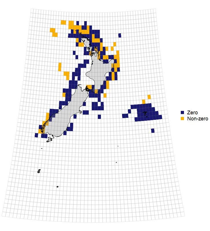
Spatial stratification based on the proportion of non-zero hāpuku/bass catch events
regardless of target species

Regression tree modelling partitioned the gridded cells where bottom longline fishing had occurred in
six strata that explained most of the variation in the proportion of non-zero catch events, regardless of
the reported target species (Figure 6). The environmental variables that explained spatial differences in
predicted catch rates were (in order): seafloor temperature, tidal current velocity, bathymetry, dynamic
topography (bathymetric variability), and seafloor rugosity (Table 4).

Figure 6: Regression tree partitioning of gridded cells based on the proportion of non-zero hāpuku/bass
 catch fishing events occurring in each cell, given environmental conditions and fishing year
 month, for all fishing events regardless of target species. ‘No’ = zero-catch fishing event strata;
 ‘Yes’ = non-zero (i.e. positive) catch event strata. Bottemp = seafloor temperature; tidalcurr =
 tidal current velocity; bathy = bathymetry; dynoc = dynamic topography; rugosity = seafloor
 rugosity.

14 • Feasibility of fishery independent longline survey designs Fisheries New Zealand

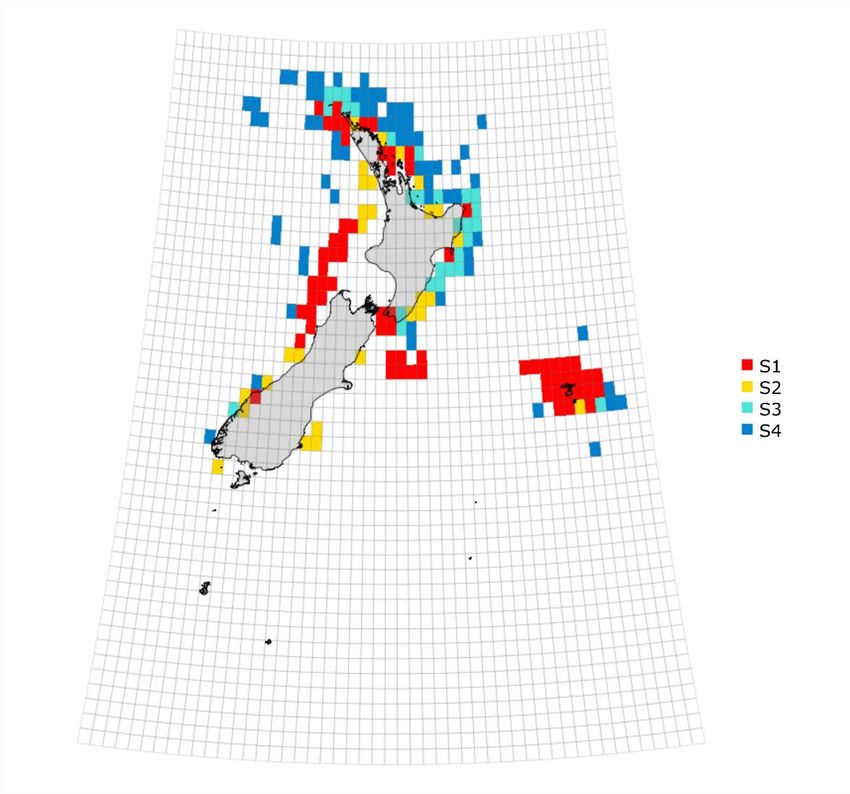
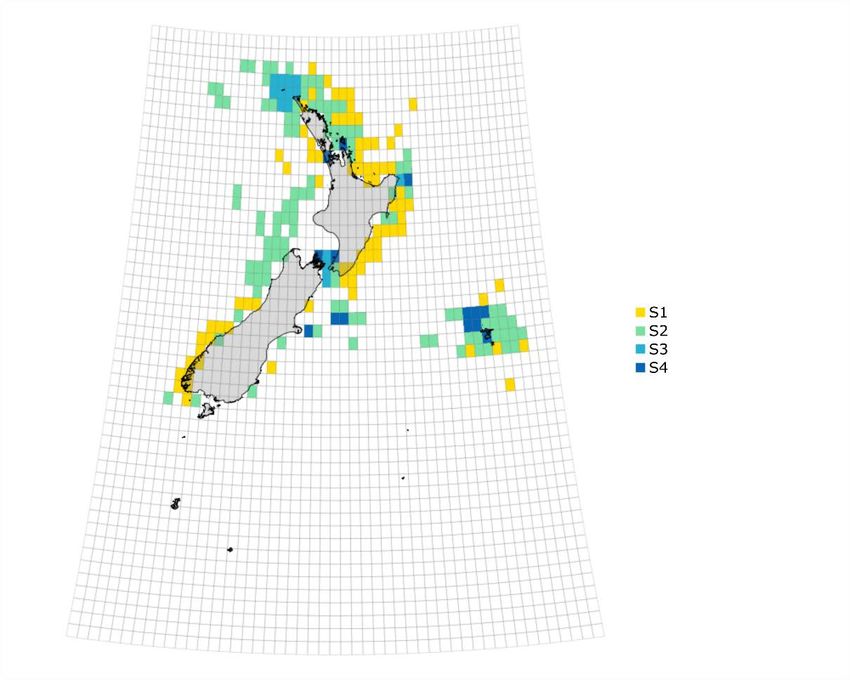
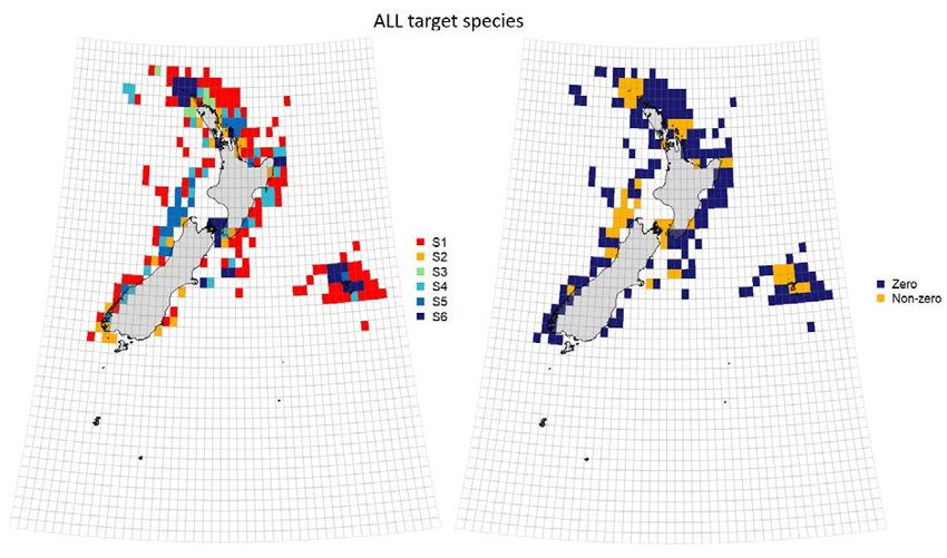
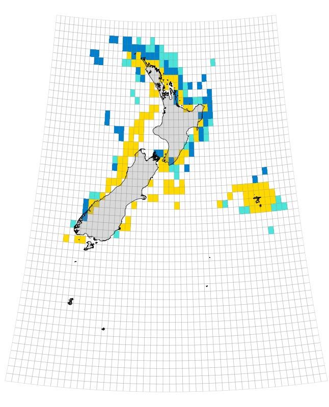
The spatial distribution of cells assigned to each stratum by the regression tree model is shown in
Figure 7. Tidal current velocities and seafloor slopes calculated at the location of fishing events within
each cell led to predicted low or zero catch fishing events for four of the six regression tree
classifications (S1, S2, S3, and S4). Trends in hāpuku/bass abundance could therefore be monitored by
a stratified longline survey conducted in those areas where non-zero catches were predicted
(classifications S5 and S6), but broad contiguous survey strata cannot be inferred from the heterogenous
spatial distribution of these two classifications. Environmental variable data were not available for a
small number of the grid cells seen in Figure 5, such northwest of the Cook Strait, and catch rate
predictions were therefore not possible for these locations.

Figure 7: Spatial distribution of gridded cells assigned to one of six strata by regression tree modelling of
 the proportion of non-zero hāpuku/bass catch events occurring in each cell, regardless of target
 species. Strata S5 and S6 in the left figure correspond to the ‘Non-zero’ cells (orange) in the right
 figure.

Spatial stratification based on the proportion of non-zero hāpuku/bass catch events
where core species were targeted

Any interpretation of the relative abundance of hāpuku and bass that is based on fishing events that
target these species, or bluenose target events that often result in catches of hāpuku or bass, should be
more accurate than one based on fishing events targeting other species. Regression tree modelling was
therefore used to spatially classify gridded cells based on predictions of the incidence of positive catch
events when these species were targeted by bottom longline, based on fishing year, month, and the
spatially explicit environmental variables given in Table 4.

The regression tree partitioned gridded cells into four classes, based on the three environmental
variables that best explained the observed incidence of non-zero hāpuku/bass catch events in each cell
(Figure 8). The three environmental variables that were selected were (in selection order): tidal current
velocity, suspended particulate matter, and seafloor salinity concentration.

Fisheries New Zealand Feasibility of fishery independent longline survey designs • 15

Size of tree

Figure 8: Regression tree partitioning of gridded cells based on the proportion of non-zero hāpuku/bass
 catch fishing events occurring in each cell, given environmental conditions and fishing year
 month, when hāpuku, bass or bluenose were targeted. ‘No’ = zero-catch fishing event strata;
 ‘Yes’ = non-zero (i.e. positive) catch event strata. Tidalcurr = tidal current velocity; susp =
 suspended particulate matter; botsal = seafloor salinity concentration.

16 • Feasibility of fishery independent longline survey designs Fisheries New Zealand

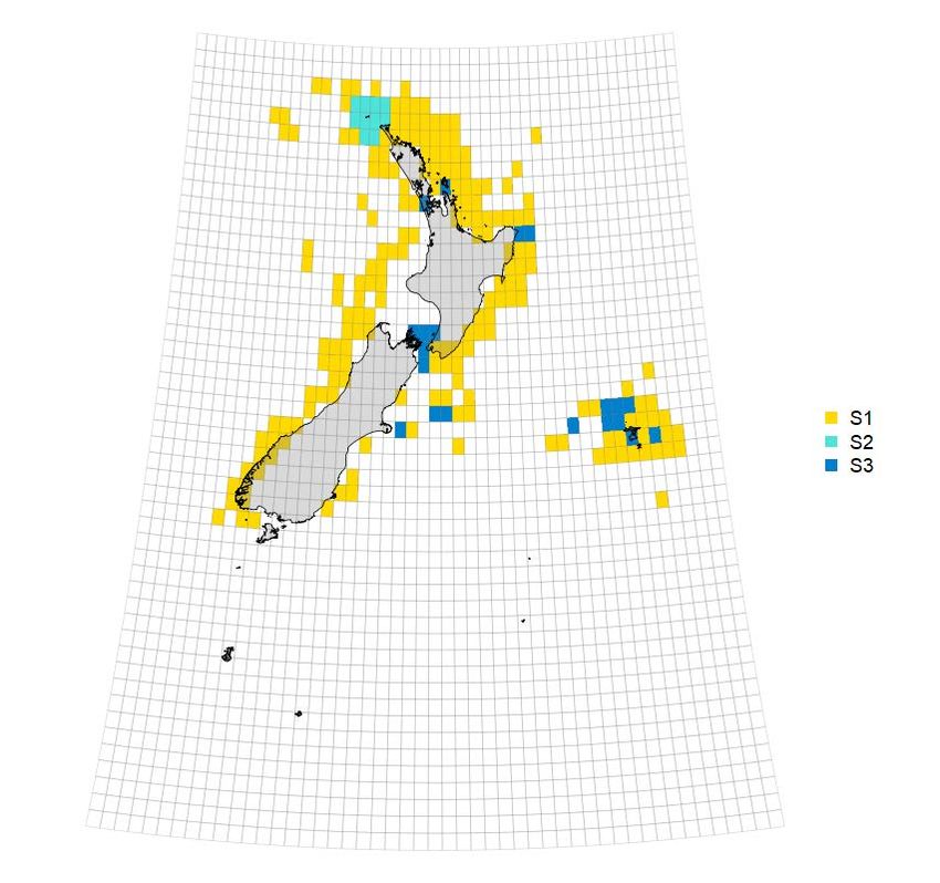
The distributions of the catch cell classifications produced by the regression tree analysis of core fishing
events (Figure 9) are more spatially homogeneous than those based on the classification of all fishing
events (see Figure 7). The resulting clusters of co-classified cells can be used to intuitively delineate
survey strata covering large contiguous areas of likely hāpuku/bass habitat. Delineated survey stratum
boundaries could exclude isolated areas classified as S1, because the catch effort data suggest that few
if any hāpuku or bass are likely to occur in these areas.

 CORE target species (HPB, BAS, HPB, BNS)

Figure 9: Spatial distribution of gridded cells assigned to one of four strata by regression tree modelling of
 the proportion of non-zero hāpuku/bass catch events occurring in each cell, based on those events
 where hāpuku, bass, or bluenose were targeted. Strata S2, S3, and S4 in the left figure correspond
 to the ‘Non-zero’ cells (orange) in the right figure.

The following two analyses focus on grid cells where at least one non-zero catch event had occurred.
The abundance of hāpuku/bass in each gridded cell was calculated as the average catch rate for all
events occurring within each cell and this was then scaled by the proportion of the area in each cell that
overlapped the seafloor. The natural logs of these calculated abundances were used for the regression
tree modelling.

Fisheries New Zealand Feasibility of fishery independent longline survey designs • 17

Spatial stratification based on averaged hāpuku/bass catch rates ― all target species

Regression tree modelling of averaged catch rates in cells where at least one non-zero hāpuku/bass catch
event had occurred, regardless of target species, partitioned the gridded cells into three groups
(Figure 10). The environmental variables that best explained the differences between these averaged
catch rates were tidal current speed and seafloor oxygen concentration, but almost all cells were
assigned to the S1 classification (Figure 11). This would suggest that there would be little to gain, in
terms of estimate precision, if a longline survey was stratified on the basis of this classification.

 Size of tree

Figure 10: Regression tree partitioning of gridded cells on the basis of an averaging of hāpuku/bass catch
 rates occurring in each cell where at least one non-zero hāpuku/bass catch event occurred,
 regardless of the target species, given environmental conditions in each gridded cell. Tidalcurr
 = tidal current speed; botoxy = seafloor oxygen concentration.

18 • Feasibility of fishery independent longline survey designs Fisheries New Zealand

Figure 11: Spatial distribution of gridded cells assigned to one of three strata by regression tree modelling
 of averaged hāpuku/bass catch rates reported in those cells where at least one non-zero catch
 event had occurred, for events where any species was targeted. Stratum S1 corresponds to the
 lowest catch rates; stratum S3 corresponds to the highest catch rates.

Fisheries New Zealand Feasibility of fishery independent longline survey designs • 19

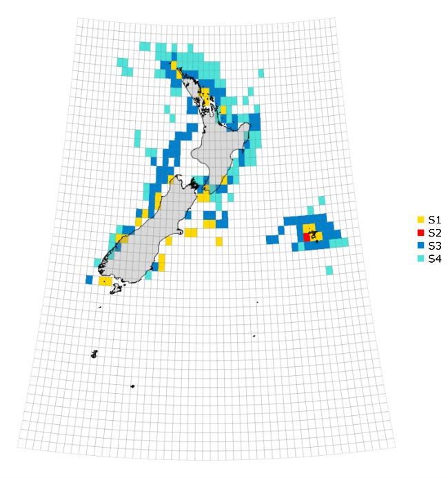
Spatial stratification based on averaged hāpuku/bass catch rates ― core target species

Regression tree modelling of averaged hāpuku/bass catch rates, for those cells where hāpuku/bass were
caught when targeting hāpuku, bass, or bluenose, partitioned the gridded cells in four classes
(Figure 12). Neighbouring cells were commonly assigned the same classifications, from which up to
ten contiguous survey strata could easily be delineated (Figure 13). Tidal current speed (split at two
levels) is once again the best predictor of catch, followed by seafloor oxygen concentration.

 Size of tree

Figure 12: Regression tree partitioning of gridded cells on the basis of an average of hāpuku/bass catch
 rates occurring in each cell where at least one non-zero hāpuku/bass catch event occurred where
 hāpuku, bass, or bluenose were targeted, given environmental conditions in each gridded cell.
 Tidalcurr = tidal current speed; botoxy = seafloor oxygen concentration.

20 • Feasibility of fishery independent longline survey designs Fisheries New Zealand

Figure 13: Spatial distribution of gridded cells assigned to one of four strata by regression tree modelling
 of averaged hāpuku/bass catch rates reported in those cells where at least one non-zero catch
 event had occurred, where hāpuku, bass, or bluenose was targeted. Stratum S4 corresponds to
 the highest expected catch rates, followed by S2, S3, and S1 (in decreasing order).

Comparison of predicted levels of precision achieved under different survey designs

The relative benefits of each of the four stratification strategies described above were assessed by using
Neyman allocation to optimally allocate sampling effort across the regression tree partitioned strata in
each case, for three levels of overall effort (50, 100, and 150 longline sets across all strata).

 ( ℎ × ℎ )
 ℎ = ×
 ∑( × )

Where nh is the number of samples allocated to stratum h, n is the total sample size to be allocated, Ni
is the population size for stratum h and Sh is the standard deviation of the catch rates calculated from
fishing events occurring in stratum h. The denominator sums over all strata.

Coefficients of variation were calculated for each of the four survey designs, based on the number of
longline sets allocated to each stratum for each of the five years for which stratum-specific summary
catch rate data were available. Coefficients of variation are also given for unstratified survey designs,
for all fishing events and for those where only core species were targeted (HAP, BAS, HPB, or BNS)
(Table 5).

Fisheries New Zealand Feasibility of fishery independent longline survey designs • 21

Table 5: Ranges of fishing year coefficients of variation calculated from alternative hāpuku/bass survey
 designs for three levels of overall effort (50, 100, and 150 longline sets across all strata). The term
 “delta” refers to analyses based on the proportion of non-zero catch events occurring in each grid
 cell. Min. is minimum CV; Max. is maximum CV.

N = 50 sets
 2014 2015 2016 2017 2018 Min. Max. Mean Median
 All target species delta 0.91 0.96 1.33 4.27 0.95 0.91 4.27 1.69 0.96
 All target species 0.36 0.40 0.61 2.33 0.35 0.35 2.33 0.81 0.40
 Core target species
 delta 0.16 0.17 0.24 0.97 0.16 0.16 0.97 0.34 0.17
 Core target species 0.13 0.15 0.22 0.88 0.14 0.13 0.88 0.31 0.15
 No stratification 0.39 0.46 0.61 2.02 0.45 0.39 2.02 0.79 0.46

N = 100 sets
 2014 2015 2016 2017 2018 Min. Max. Mean Median
 All target species delta 0.59 0.65 0.90 2.86 0.63 0.59 2.86 1.13 0.65
 All target species 0.25 0.28 0.42 1.67 0.25 0.25 1.67 0.57 0.28
 Core target species
 delta 0.11 0.12 0.17 0.69 0.11 0.11 0.69 0.24 0.12
 Core target species 0.10 0.11 0.15 0.62 0.10 0.10 0.62 0.22 0.11
 No stratification 0.28 0.32 0.44 1.36 0.32 0.28 1.36 0.54 0.32

N = 150 sets
 2014 2015 2016 2017 2018 Min. Max. Mean Median
 All target species delta 0.46 0.50 0.73 2.37 0.50 0.46 2.37 0.91 0.50
 All target species 0.20 0.23 0.35 1.36 0.20 0.20 1.36 0.47 0.23
 Core target species
 delta 0.09 0.10 0.14 0.57 0.09 0.09 0.57 0.20 0.10
 Core target species 0.08 0.09 0.13 0.51 0.08 0.08 0.51 0.18 0.09
 No stratification 0.22 0.26 0.35 1.15 0.26 0.22 1.15 0.45 0.26

These analyses suggested that:

 • Designs for a national survey, based on a regression tree classification of locations where one
 of the core species was targeted are likely to produce more precise relative abundance estimates
 than those based on an analysis of all available fishing events, regardless of which species were
 targeted.
 • Stratified survey designs are more likely to produce precise estimates than unstratified survey
 designs.
 • At least 50 longline sets would be required to produce a reasonably precise survey abundance
 estimate, but this level of sampling effort may not be sufficient in some years, based on the
 range of CV estimates calculated from the catch effort data available for each of the last five
 complete fishing years.

Feasibility of a bottom longline survey of the HPB 1 stock

The survey precision estimates given in Table 5 suggest that only 50 longline sets would be required to
monitor trends in hāpuku/bass abundance, to achieve an expected median CV < 0.30. Despite this, there
are several reasons why a larger sample size would be required to confidently achieve an acceptable
level of precision. Firstly, because the derived CVs are based on combined hāpuku and bass catch rate
data, a survey design aimed at estimating abundance for each species separately is likely to require
significantly more longline sets to achieve a target CV of 0.30 for each species. It may be hard to
consistently achieve acceptably precise survey CVs for each species if a survey is designed to monitor
the abundance of each species simultaneously, because the relative abundance of hāpuku vs. bass in
any given area is likely to differ over time, because of differences in environmental conditions and

22 • Feasibility of fishery independent longline survey designs Fisheries New Zealand

fishing pressure in their respective depth ranges (bass are more commonly caught in the north and in
shallower waters than hāpuku).

Secondly, because New Zealand waters support several hāpuku/bass stocks (which are managed as
eight distinct HPB stocks under the QMS) and trends in the abundance of each stock will vary over
time, they should not be regarded as a single national stock that could be monitored by a single survey.
Thirdly, because the size of the commercial fleet is limited, it would therefore be unable to provide the
capacity required for such an extensive and logistically intensive national survey (which would also be
beyond the capacity of New Zealand’s limited research vessel fleet).

An alternative option to a nation-wide survey would be to conduct a smaller scale longline survey of
one or two high priority HPB fish stocks, to both monitor trends in hāpuku and bass abundance, and to
assess the feasibility of this monitoring approach. This option was explored, for the HPB 1 stock, which
supports New Zealand’s largest hāpuku/bass longline fishery, in terms of annual tonnage landed
(approximately 200 t per annum ― see Figure 3). The spatial extent of the HPB 1 stock was therefore
subdivided into three strata, based on a cursory examination of the spatial distribution of hāpuku/bass
fishing effort and catch rates in each of the last five fishing years (Figure 14).

Figure 14: Definitions of three survey strata for HPB 1 given geographical constraints and a cursory
 examination of the spatial distribution of hāpuku/bass catch rates during each of the last five
 fishing years.

Estimates of bottom longline survey abundance estimate precision were then calculated for a three strata
survey of HPB 1:
 • based on all available catch and effort data from those events where hāpuku or bass was caught,
 regardless of target species.

Fisheries New Zealand Feasibility of fishery independent longline survey designs • 23

• based on all available catch and effort data from those events where hāpuku or bass was caught,
 where the reported target species was either HAP, BAS, HPB or BNS.

These analyses suggest that as few as 30 longline sets might be required to produce a reasonably precise
average catch rate estimate for this northern area of HPB 1 (hāpuku and bass combined) in any given
year, but the precision estimates for 2017 are low, so a greater number of sets should be considered to
allow for interannual variability in catch rates (Table 6). The HPB 1 simulated survey CVs were higher
than the national survey CVs (Table 5) for the same number of stations, which suggests that the within-
area sample variation of HPB 1 is greater than the overall inherent variation of the combined area
national survey. Once again, it should be noted that these precision estimates are based on non-random
targeted fishing events and may therefore overestimate the precision that might be achieved by a fully
randomised survey.

Table 6: Ranges of fishing year coefficients of variation calculated from alternative designs for a bottom
 longline survey of the HPB 1 stock only. Min. is minimum CV; Max. is maximum CV.

N = 30 sets
 2014 2015 2016 2017 2018 Min. Max. Mean Median
 3 strata - all target spp 0.21 0.22 0.33 1.32 0.23 0.21 1.32 0.46 0.23
 3 strata - core target
 spp 0.18 0.19 0.30 1.22 0.20 0.18 1.22 0.42 0.20

N = 50 sets
 2014 2015 2016 2017 2018 Min. Max. Mean Median
 3 strata - all target spp 0.16 0.17 0.26 1.03 0.18 0.16 1.03 0.36 0.18
 3 strata - core target
 spp 0.14 0.15 0.23 0.94 0.15 0.14 0.94 0.32 0.15

Commercial hāpuku/bass longline skippers were subsequently interviewed, to gauge the logistical
feasibility of a 50 plus station HPB 1 survey. Interviews with three bottom longline skippers who
currently account for most of the hāpuku/bass catch taken from this stock are given in Appendix 3 (see
Fishers J, K, & L). These fishers were asked to describe the fishing gear that they used, to inform the
specification of a standardised longline design (as summarised at the beginning of Appendix 3), and
about any aspects of their fishing practice that may have a direct bearing on the design of a longline
survey. A key conclusion of these interviews was that no more than two sites could be surveyed per
day, and even this would only be possible when there were two survey sites within 10 nautical miles of
each other. This is because longlines are usually deployed over a short period between midnight and
dawn to maintain consistently reliable catch rates, which would be an important consideration for any
longline survey. The spatial spread of surveyed sites would therefore determine the number of days
required for such a survey, and hence its cost effectiveness and feasibility given normal commercial
fishing operational requirements.

The most experienced of these skippers was asked to propose survey strata for the areas that he had
previously fished in HPB 1, which covered most, but not all, of the potential hāpuku/bass habitat in
Northern HPB 1. Although the spatial extent of this fisher’s experience only covered the northern half
of HPB 1, the degree to which he stratified this area (Figure 15) and the justification that he gave for
this level of stratification, in terms of catch rates and the hāpuku/bass species mix (Table 7), can be
used to assess the feasibility of a longline survey conducted at even this reduced spatial extent.

If the minimum number of longline sets required to produce a reasonably precise average catch rate
estimate is 50 sets, and these sets are randomly allocated across the five strata shown in Figure 15, in
proportion to the area of each stratum, the distances between each set limits the number of instances
where two longline sets could be deployed during the same period of darkness. This means that a
minimum of 36 days would be required for a longline survey of this sub area of HPB 1 under this

24 • Feasibility of fishery independent longline survey designs Fisheries New Zealand

scenario, regardless of the time required to access these survey strata from the nearest port, as well as
any downtime allowed for unfishable weather. This would suggest that a bottom longline survey is
unlikely to be a viable means of monitoring hāpuku/bass abundance at any meaningful spatial scale,
especially given the limited scale of the commercial fishery that could support such a survey.

Figure 15: Bottom longline survey strata defined by an experienced HPB 1 commercial bottom longline
 fisher, given the spatial distribution of expected catch rates and the relative mix of hāpuku and
 bass in each area, as given in Table 7. Numbers denote the location of a set of randomly
 generated survey stations and circles denote pairs of survey stations that could be surveyed on
 the same day given logistical constraints.

Table 7: Expected catch rates and the mix of hāpuku/bass in each of the five strata indicated in Figure 15.

 Stratum ID Catch rate per hook Species catch mix
 A 0.25 to 0.5 kg 80% bass 20% hāpuku
 B 0.5 to 1 kg 20% bass 80% hāpuku
 C 0.5 to 1 kg 70% bass 30% hāpuku
 D 0.1 to 0.25 kg 30% bass 70% hāpuku
 E 0.25 to 0.5 kg 30% bass 70% hāpuku

There are other reasons why a bottom longline survey monitoring approach might be potentially
unreliable, such as the hyperstability of catch rates of species that aggregate around localised seafloor
structures targeted by longliners, to maintain commercially viable catch rates, and the uncertain reliance
on a commercial fisher to undertake such a survey in a consistent fashion over the long term.

An alternative approach to monitoring hāpuku/bass stocks ― catch sampling

Although a bottom longline survey does not appear to be a feasible way of monitoring trends in the
abundance of hāpuku/bass at an appropriate management scale, there is a viable alternative monitoring
approach that could be used. Otoliths are routinely collected and aged from commercial and recreational
landings of other species, to determine the average relative rate at which recruited year classes in an age

Fisheries New Zealand Feasibility of fishery independent longline survey designs • 25

distribution decline over time (i.e., total mortality rate), which can be interpreted as a proxy measure of
change in stock status. Examples of where this catch curve approach has been used to monitor the status
of other species include sampling of recreational kingfish landings (Holdsworth et al. 2013) and a
current jack mackerel Trachurus novaezelandiae purse seine catch sampling programme
(JMA2018/01). Francis et al. (1999) used oxytetracycline injection trials to validate the annual
deposition of annual opaque hyaline zones in hāpuku otoliths, and these ageing methods were
subsequently used by Parker et al. (2011).

Catch sampling for age is potentially a more cost-effective monitoring approach for HBP stocks,
because the costs associated with shed sampling and otolith preparation and ageing are far less than
those associated with chartering a fishing vessel to set and retrieve longline gear at only one or two sites
per day. Catch sampling can also be used to monitor the stock status of hāpuku and bass separately, if
landings of both species are targeted in a coordinated fashion. The viability of this approach would be
dependent on the degree of cooperation provided by the small number of longline fishers participating
in a monitored hāpuku/bass longline fishery, given the relatively small number of landings that are
likely to be available, so that targeted sampling and prior information of the species mix in these
landings is possible.

The possibility of deriving catch curve total mortality estimates from otoliths collected by observers
was investigated by Parker et al. 2011, and although this approach was not considered viable because
of the limited number of otoliths collected by observers at that time, the authors did suggest an
alternative commercial landing catch sampling approach, such as that proposed here.

Regardless of the monitoring method used, the size composition hāpuku and bass associated with
specific seafloor structures varies over time, with specific size ranges being associated with different
features during the spawning season, and more random mixing of the population occurring across
features at other times (Adam Davey, HPB 1 commercial longline fisher, pers. comm.). Cooperation
with longline fishers will therefore be required to ensure the consistent targeting of predefined
“sentinel” features over a given period each year, to improve the comparability of catch curves total
mortality estimates over time. The timing of this catch sampling period is also an important
consideration. Catch sampling should occur outside the spawning season for several reasons. Catch
rates during the spawning season are unpredictable, with the fish often not biting despite gear being set
over known aggregations several times before they are caught in any abundance. Catch sampling
outside the spawning season is also more likely to provide a consistent sample from a fish stock, because
the more random degree of mixing at these times means that fish are more likely to have a homogeneous
selection probability, regardless of their spawning condition or size. Changes in the relative influence
of each sentinel feature, in response to changes in stock status and as a result any short-term localised
depletion caused by another recent fishing event on the same feature, will also be less of a concern,
because the relative contribution of the catch taken across a group of features is more likely to be self-
weighting when random mixing occurs outside the spawning season.

2.3 Longline survey design for bluenose

The methods used to evaluate the feasibility of a national longline survey for bluenose closely follow
that used above for hāpuku/bass. All five of the commercial bottom longline fishers who were
interviewed about their hāpuku/bass fishing activity were asked whether it would be possible to extend
a hāpuku/bass longline survey to also monitor trends in bluenose abundance. None of these interviewed
fishers thought that a combined hāpuku/bass and bluenose longline survey would be feasible because
there was too much difference between the gear used and areas or depths fished for bluenose, despite
the fact that one of these species was often caught when targeting the other. The following analyses
were therefore undertaken to explore the feasibility of a dedicated national bluenose longline survey.

26 • Feasibility of fishery independent longline survey designs Fisheries New Zealand