Sector models-A toolkit for teaching general relativity: II. Geodesics
←
→
Page content transcription
If your browser does not render page correctly, please read the page content below
Sector models—A toolkit for teaching general
arXiv:1804.09828v1 [physics.ed-ph] 25 Apr 2018

                                                 relativity: II. Geodesics
                                                         C Zahn and U Kraus

                                                         Institut für Physik, Universität Hildesheim, Universitätsplatz 1, 31141 Hildesheim,
                                                         Germany
                                                         E-mail: corvin.zahn@uni-hildesheim.de, ute.kraus@uni-hildesheim.de

                                                         Abstract.
                                                         Sector models are tools that make it possible to teach the basic principles of the general
                                                         theory of relativity without going beyond elementary mathematics. This contribution
                                                         shows how sector models can be used to determine geodesics. We outline a workshop for
                                                         high school and undergraduate students that addresses gravitational light deflection
                                                         by means of the construction of geodesics on sector models. Geodesics close to a
                                                         black hole are used by way of example. The contribution also describes a simplified
                                                         calculation of sector models that students can carry out on their own. The accuracy of
                                                         the geodesics constructed on sector models is discussed in comparison with numerically
                                                         computed solutions. The teaching materials presented in this paper are available online
                                                         for teaching purposes at www.spacetimetravel.org.

                                                         Keywords: general relativity, geodesics, black hole, gravitational light deflection, sector
                                                         models
Sector models: II. Geodesics 2
1. Introduction
To teach the basic principles of the general theory of relativity without going beyond
elementary mathematics remains a challenge even a century after the completion of
the theory. In view of this objective, we describe a novel approach that is focussed
on geometric insight and makes do with elementary mathematics as taught in school.
This approach is suitable for learners who lack the qualifications or the time required
to master the mathematical tools that are needed for a standard introductory text, i.e.,
advanced high school students and undergraduate students, especially those in a physics
minor programme or in physics teacher education. The approach can also be used as a
supplement to standard textbooks (e.g., Hartle 2003) to strengthen geometric insight.
In a first paper (Zahn and Kraus 2014, in the following referred to as paper I), we
have developed sector models as a new type of physical model for curved spaces and
spacetimes. We have shown how they can be used to convey the notion of a space
or a spacetime being curved. In paper I, sector models were first introduced for two-
dimensional curved surfaces of positive or negative curvature. They were then developed
for three-dimensional curved spaces and 1+1-dimensional curved spacetimes using the
Schwarzschild black hole as an example.
Sector models implement the description of curved spacetimes used in the Regge
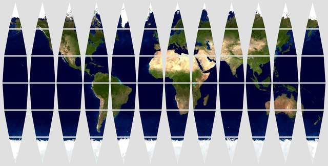
calculus (Regge 1961) in the form of physical models. Figure 1 illustrates the basic
principle using the surface of the earth by way of example: The surface is approximated
by means of small flat elements of area. When these are laid out in the plane, one
obtains a world map; this map is the sector model of the surface of the earth. Two
differences to ordinary world maps stand out: The sector map is non-contiguous, since
it is not possible to join all sectors simultaneously to all their neighbours. Also, the
sector map is undistorted within the bounds of the discretization error, preserving both
lengths and angles. It is, therefore, open to an intuitive geometric understanding. The
sector model of a curved three-dimensional space is built along the same lines. The flat
elements of area are replaced by blocks with euclidean geometry. In the case of a curved
spacetime, the sectors are spacetime blocks with Minkowski geometry.
The general theory of relativity describes the paths of light and of free particles as
geodesics of a curved spacetime. The notion of geodesics, therefore, is an important point
in any introduction to general relativity. This contribution shows how sector models
can be used to introduce the concept of geodesics and to determine geodesics by graphic
construction. Instead of solving a system of ordinary differential equations, geodesics
are constructed with pencil and ruler. The construction implements the description
of geodesics in the Regge calculus (Williams and Ellis 1981) and gives quantitatively
correct results (within the discretization error).
In this contribution, we outline a workshop on gravitational light deflection the
way we teach it for high school and for undergraduate students (section 2). Section 3
is a discussion of the approximations involved in the construction of geodesics on sector
models and a study of the accuracy that can be achieved. Conclusions and outlook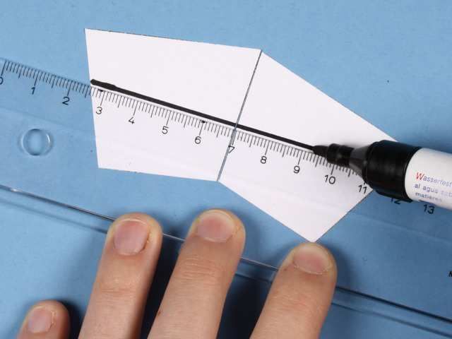
Sector models: II. Geodesics                                                               3

               Figure 1. Sector model of the surface of the earth. Earth texture: NASA.

follow in section 4.

2. Workshop on geodesics and light deflection

The workshop starts by introducing the concept of geodesics, using curved surfaces by
way of example. Geodesics are then constructed on the sector model of a black hole
in order to show how gravitational light deflection arises. The black hole is used as an
example because close to it relativistic effects are large and, therefore, clearly visible in
the graphic constructions. As an extension to the workshop, we describe a simplified
procedure for the calculation of sector models that students can use to create sector
models on their own. This enables them to study the geodesics of a spacetime starting
from a given metric.

2.1. Geodesics on curved surfaces
The introduction to the workshop includes the explanation that the general theory of
relativity describes the paths of light and of free particles as geodesics. Depending on the
background of the participants, the significance of geodesics in general relativity may just
be stated or may be explained in more detail with reference to the equivalence principle
(e.g., Natário 2011, chapter 5). In preparation for the determination of geodesics in the
vicinity of a black hole, geodesics are first studied on curved surfaces.
     The geodesic line on a curved surface is introduced as a locally straight line. Such
a line keeps its direction at each point, i.e., it neither bends nor kinks. A criterion
is described that permits to recognize a geodesic: One imagines that a narrow strip
made of a non-elastic material is glued along its centre line onto the line that is to
be investigated. If the line bends, the strip tears on the outside and buckles on the
inside—this shows that the line is not a geodesic.
     The sphere is used as the first example (figure 2). We consider a line that starts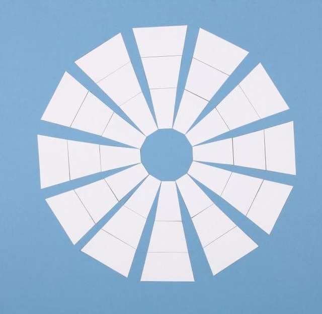
Sector models: II. Geodesics                                                                   4

              Figure 2. The geodesics on the sphere are the great circles.

               (a)                               (b)

              Figure 3. A spherical cap is approximated by facets (a) and represented as a sector
              model (b).

              Figure 4. The construction of a geodesic on a sector model.

from the equator due north and is locally straight. It is obvious that the line is a line of
longitude. The lines of longitude, and more generally all great circles, are geodesics on
the sphere. Figure 2 illustrates a characteristic property of these geodesics: Two lines of
longitude are parallel at the equator; towards the north pole they converge. Generally
speaking, geodesics on the sphere converge when starting in parallel.
     In the next step we show how this property of geodesics on the sphere can be
obtained from a sector model. A spherical cap is approximated by facets (figure 3(a)),
and the facets are laid out as a sector model (figure 3(b)). Now a geodesic is drawn
onto the sector model. Within a sector, i.e., on a flat element of area, a geodesic is
a straight line. When the line reaches the border of a sector, it is continued onto the
neighbouring sector. How to do this follows from the definition of the geodesic: locally
straight (figure 4). The two neighbouring sectors are joined at their common edge and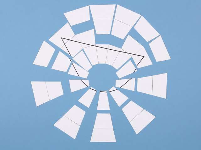
Sector models: II. Geodesics                                                                     5

(a)                             (b)                                (c)

              Figure 5. Geodesics on the sector model of a spherical cap. In (a) the sectors are
              joined along the bottom geodesic and in (b) along the top geodesic. The two geodesics
              are parallel in the bottom left sector and converge towards the right hand side ((b),
              (c)).

               (a)                               (b)

               (c)                               (d)

              Figure 6. A saddle (a) is in part approximated by facets (b) and represented as a
              sector model (c); geodesics starting parallel to each other diverge ((a), (d)).

the line is continued straight across the border. In this way the geodesic is continued
across the sector model (figure 5(a)). A second geodesic is then added that is parallel
to the first in the bottom left sector (figure 5(b)). One can see that the two geodesics
starting in parallel on the lower left converge towards the right hand side (figures 5(b),
(c)).
      A saddle is taken as a second example. Adhesive strips glued to the surface show
that geodesics starting parallel to each other diverge (figure 6(a)). The approximation
of a part of the surface by facets (figure 6(b)) leads to the sector model (figure 6(c)).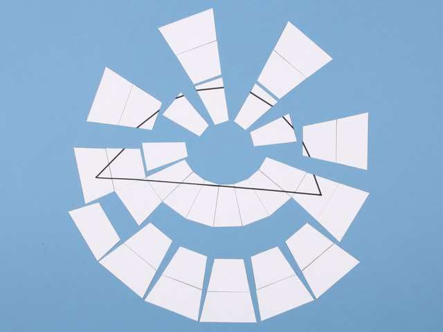
Sector models: II. Geodesics                                                                            6

(a)                                                   (b)

                 Figure 7. A thought experiment on the construction of the sector model of the
                 black hole equatorial plane: A lattice is erected around the black hole according to
                 the pattern shown in (a). For each cell, the lengths of the four enclosing rods are
                 measured and from these data paper sectors are constructed true to scale. The result
                 is the sector model of a ring around the black hole (b).

On the sector model, two geodesics are constructed that are parallel to each other in
the lower left sector; these geodesics diverge (figure 6(d)).
     The two examples show that sector models of curved surfaces can be used as tools
to study the properties of geodesics on these surfaces.

2.2. Geodesics close to a black hole
The second part of the workshop begins with the presentation of a sector model that
permits to construct geodesics in the vicinity of a black hole. The sector model represents
a plane of symmetry of the black hole that in the following we will call equatorial plane.‡
     To introduce the sector model, its ”construction” is described in a thought
experiment: A spaceship is sent to a black hole with the task of surveying the space
around it. To this end, a lattice is erected around the black hole according to the
pattern shown in figure 7(a): Rigid rods are arranged like an orb web in the equatorial
plane, centred on the black hole. The whole lattice is located outside of the event
horizon because no such static structure is possible in the inner region of the black
hole.§ Measurements are taken of the lattice: Each cell is enclosed by four rods. The
lengths of the rods are measured and the data sent to Earth. There, each cell, reduced
‡ We consider a non-rotating black hole. It has spherical symmetry, therefore, every geodesic lies in a
plane that is a symmetry plane of the black hole.
§ The lattice covers the region from 1.25 to 5 Schwarzschild radii in the Schwarzschild radial coordinate,
see section 2.4.2.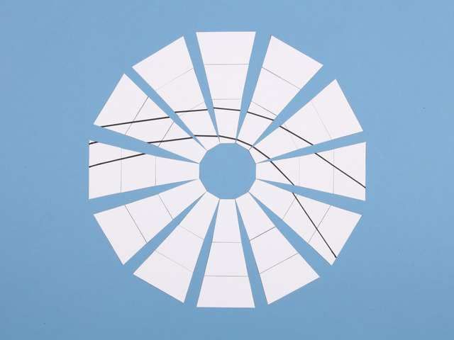
Sector models: II. Geodesics                                                                          7

                 (a)                                 (b)

                Figure 8. A geodesic on the sector model of the equatorial plane of a black hole.
                The line is locally straight; the direction ”far behind” the black hole differs from the
                direction ”far ahead”. In (a) the sectors are joined along the geodesic and in (b) they
                are arranged symmetrically.

in size, is represented by a sector. The complete set of sectors forms a true to scale
model of a ring around the black hole (figure 7(b)). Obviously, the sectors cannot be
arranged to cover a ring without leaving gaps. This indicates that the geometry of the
black hole equatorial plane is different from the geometry of the plane surface on which
the sectors are laid out. The equatorial plane of the black hole is part of a curved space;
the flat support of the model is a plane in euclidean space. If one could place a black
hole with the appropriate mass in the centre of the model, then all the flat pieces with
the sizes and shapes as shown would fit without gaps. The required mass amounts to
about three earth masses for the cut-out sheet that is provided online (Zahn and Kraus
2018).
      Alternatively, the sector model can be introduced via the workshop on curved
space described in paper I. This workshop presents a sector model of the curved three-
dimensional space around a black hole (figure 5(b) in paper I). The equatorial plane of
this model (in figure 5(b) of paper I: the green, nearly horizontal sides of the blocks) is
identical with the sector model shown in figure 7(b).
      To build the sector model shown in figure 7(b), the sectors are cut out of a sheet
of paper and are glued onto cardboard with spray adhesive (use repositionable spray
adhesive for repeated lifting and repositioning)k. The sector model is then used to study
geodesics close to a black hole. First a single geodesic is drawn across the sector model.
As in the case of the curved surfaces described above, this is done by joining neighbouring
sectors and drawing a straight line (figure 8(a)). It can be seen that the two end sections
of the line point in different directions (Fig 8(b)). Thus, for a line that passes close to a
black hole while keeping its direction at each point, the direction ”far behind” the black
hole differs from the direction ”far ahead”. This construction illustrates the principle
underlying light deflection in a gravitational field: Light propagates on a locally straight
path; when it passes a region of curved space, the direction of propagation afterwards
is different from that before.
k See section 2.3 for a method that does not require the use of adhesive.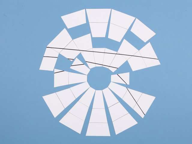
Sector models: II. Geodesics                                                                         8

               (a)                                 (b)

              Figure 9. To the geodesic shown in figure 8, a second geodesic is added that on the
              far left is parallel to the first: The inner geodesic is deflected more strongly, and the
              two geodesics diverge. In (a) the sectors are joined along the second geodesic, in (b)
              they are arranged symmetrically.

      Two things must be borne in mind when assessing the significance of this
construction on a sector model. First, the geodesics constructed on sector models
are quantitatively correct. When the condition of a locally straight line is expressed
mathematically, the result is the geodesic equation (Weinberg 1972, p. 70 ff). The
graphically constructed geodesic is a solution of this equation. Since the sector model is
an approximate representation of the curved space, the geodesic drawn on it is likewise
an approximate solution. Using an appropriately fine subdivision, geodesics can in
principle be graphically constructed with high accuracy (section 3). Secondly one must
bear in mind that though the line constructed above is a geodesic, it is not a light ray.
This line is a geodesic in space. But light propagates in space and time, meaning that
light rays are spacetime geodesics. Nevertheless, the geodesic in space illustrates by way
of close analogy the principle behind gravitational light deflection.
      Even though geodesics in space are not identical with light rays, it is instructive
to use them for demonstrating properties of geodesics. One may for instance construct
a second geodesic that starts close to the first and in the same direction (figure 9).
The geodesic that runs closer to the black hole is deflected more strongly and the two
geodesics diverge. Or one may construct two geodesics that come from the same point,
pass the black hole on opposite sides, and meet again (figure 10). Thus, with geodesics
it is possible to form a digon. Extrapolated to light rays, this construction shows how
double images arise.

2.3. The construction of geodesics using transfer sectors
Figures 8, 9, and 10 show sectors that have been cut out of a sheet of paper and have been
aligned along a geodesic or arranged symmetrically, as required. This procedure has the
advantage that each geodesic can separately be displayed as a straight line. However,
the construction of geodesics can be carried out more easily and more quickly without
cutting out all the sectors. To this end, one uses the complete model in symmetric layout
and with tick marks as shown in figure 11(a). A single additional column (figure 11(b))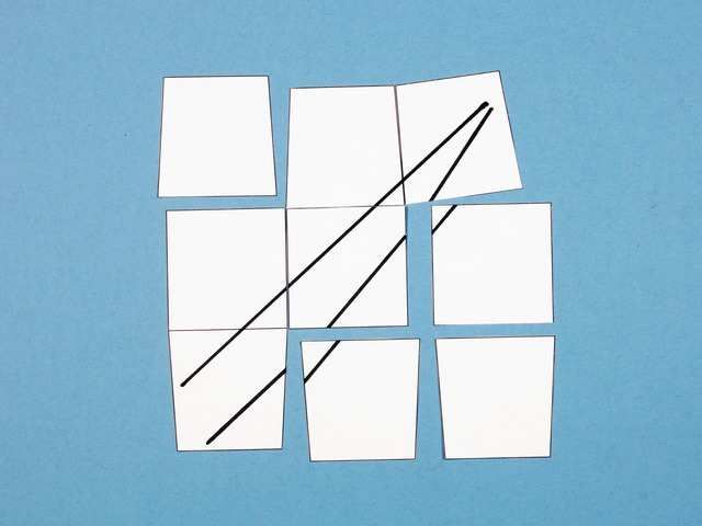
Sector models: II. Geodesics                                                                         9

(a)                              (b)                                 (c)

              Figure 10. Two geodesics form a digon. This illustrates the formation of double
              images due to gravitational light deflection: Light emitted from a source reaches the
              observer along two different paths. In (a) and (b) the sectors are joined along the first
              and the second geodesic, respectively, in (c) they are arranged symmetrically.

                                                                                 rS

            (a)                                                            (b)

              Figure 11. Worksheet for the construction of geodesics close to a black hole. The
              worksheet includes the sector model of the equatorial plane arranged symmetrically
              and with tick marks (a) and a column of transfer sectors (b). The length of the scale
              bar indicates the Schwarzschild radius rS of the black hole.

is cut out of a sheet of paper, these are the so-called transfer sectors. The construction
of a geodesic starts on the symmetric model and the line is first drawn up to the border
of the column (figure 12(a)). The appropriate sector of the transfer column is then
joined and the line is continued across the column of transfer sectors (figure 12(b)). The
line on the transfer column is copied onto the neighbouring column of the symmetric
model (figure 12(c)). This procedure is repeated up to the desired end point. In the
model shown in figure 11(a), equidistant tick marks have been added at the borders to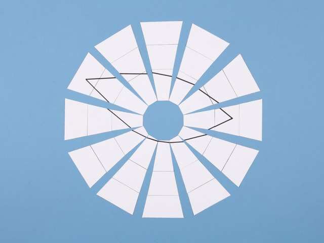
Sector models: II. Geodesics                                                                  10

(a)                               (b)                          (c)

              Figure 12.      The construction of geodesics using transfer sectors (coloured). A
              geodesic is drawn up to the border of the column (a), continued across the transfer
              column (b), and copied from the transfer column onto the neighbouring column (c).

facilitate the copying of the lines. The worksheet shown in figure 11 is available online
(Zahn and Kraus 2018).

2.4. The construction of sector models
A workshop can be implemented as described above, with sector models that are
provided. This is the most elementary and the shortest type of workshop. But for sector
models to realize their full potential as tools for studying curved spaces, the participants
should calculate and construct the models on their own. This enables them to study
other curved spaces in the same way, by, e.g., studying the geodesics corresponding to a
given metric. Thus, setting up and solving the geodesic equation is replaced by creating
the sector model and drawing the geodesics onto it.
     The following section shows how one may introduce the calculation of sector models
by using the sphere as an example. This procedure is then extended to the calculation
of the sector model of the black hole equatorial plane.

2.4.1. Construction of the sector model of a spherical surface. This example serves to
introduce the general procedure for the construction of sector models. The starting point
is the concept of a metric as a function that takes the coordinates of two nearby points
as arguments and returns their distance. This can be introduced in an elementary way
by starting with curvilinear coordinates in the euclidean plane (e.g., Kraus and Zahn
2016; Hartle 2003, p. 21 f; Natário 2011, p. 35 f).
     For the sector model of the sphere, the calculation is based on the metric in the
usual spherical coordinates θ, φ (figure 13(a)):
              ds2 = R2 dθ2 + R2 sin2 θ dφ2 ,                                                 (1)
where R is the radius of the sphere (for an elementary derivation that can be used in
the workshop, see, e.g., Hartle 2003, p. 23 f; Natário 2011, p. 37 ff).
     The creation of the sector model proceeds in three steps. In the first step the sphere
is divided up into elements of area, defined by their vertices. In the example shown here,
Sector models: II. Geodesics 11
0 π/9 φ
0
π/3
2π/3
θ
(a) (b) (c)
Figure 13. (a) The sphere described in polar coordinates θ, φ and subdivided into
elements of area of 20 degrees by 20 degrees. (b) Three elements of area in φ-θ
coordinate space. (c) The corresponding sectors. They make up one column of the
model shown in figure 3(b). For clarity, one and the same sector is highlighted in grey
in all three component images.
the elements of area are quadrilaterals with vertices at 20 degree (π/9) intervals in the
angular coordinates θ and φ, respectively (figures 13(a), (b)). In the second step the
edge lengths of the quadrilaterals are computed. This is done in an approximate way
in order to keep the calculation simple. For each edge, one determines the length by
treating the end points as nearby points in the sense of the metric. For edges between
vertices with the same longitude, one obtains the length
∆s = R ∆θ (∆φ = 0), (2)
in this example ∆s = Rπ/9. For edges between two vertices of the same latitude, one
finds
∆s = R sin θ ∆φ (∆θ = 0), (3)
depending on the angle θ of the circle of latitude. For the sector models shown in
the figures and provided online, the distance between vertices is determined along
geodesics (see paper I). The difference between the approximate and the exact edge
lengths amounts to 0.13% at most in this example.
In step three flat pieces of area are constructed from the edge lengths. In the present
example, the elements of area on the sphere possess mirror symmetry. The flat pieces
of area are constructed with the same symmetry property in the shape of symmetric
trapezia (figure 13(c)).
2.4.2. Construction of the sector model of the equatorial plane of a black hole. The
starting point of the calculation is the metric of the equatorial plane of a black hole
1
ds2 = dr 2 + r 2 dφ2 (4)
1 − rS /rSector models: II. Geodesics 12
r
5 rS
3.75 rS
2.5 rS
1.25 rS
0
0 π/6 φ
(a) (b)
Figure 14. Construction of the sector model of the equatorial plane of a black
hole. (a) The three elements of area of one column in φ-r coordinate space. (b)
The corresponding sectors.
with the usual Schwarzschild coordinates r and φ. Here, rS = 2GM/c2 is the
Schwarzschild radius of the black hole with mass M, G is the gravitational constant,
and c the speed of light. The sector model represents an annular part of the equatorial
plane, centred on the black hole. The inner rim is located at r = 1.25 rS and the outer
rim at r = 5 rS . The azimuthal angle φ has values between zero and 2π.
First the ring is divided up into elements of area. For that purpose, the φ-range is
subdivided into twelve segments of coordinate length π/6 each. Since the metric does not
depend on the coordinate φ, only one of the twelve segments needs to be calculated. The
r-range is subdivided into three segments of coordinate length 1.25 rS each (figure 14(a)).
Next, the edge lengths of the three quadrilaterals shown in figure 14(a) are calculated.
Using the metric, the distance between vertices with the same value of r is obtained as
∆s = r ∆φ (∆r = 0). (5)
When calculating the distance of vertices with the same φ-coordinate, the first term
of the metric comes into play. Its metric coefficient 1/(1 − rS /r) depends on r and,
therefore, varies along the edge. Here we make another approximation and use the
metric coefficient at the mean r-coordinate rm of the edge:
s
1
∆s = ∆r (∆φ = 0), (6)
(1 − rS /rm )
where rm = (r1 + r2 )/2 with the coordinates r1 and r2 of the associated vertices. The
sector models shown in the figures and provided online are constructed with edge lengths
that are computed numerically for geodesics joining the vertices. The difference between
the approximate and the exact edge lengths is largest for the innermost radial edge and
there amounts to 5.4%.
Step three is the construction of the quadrilaterals. The subdivision of the ring
by radial cuts creates elements of area that possess mirror symmetry (figure 7(a)).Sector models: II. Geodesics 13
(a) (b)
Figure 15. Two geodesics start in parallel (a), pass a vertex on opposite sides, and
are then inclined towards each other by the deficit angle (b).
In accordance with this symmetry, the sectors are constructed as symmetric trapezia.
Figure 14 shows the three sectors of a column together with the corresponding three
rectangles in φ − r coordinate space. The complete sector model with twelve columns
is shown in figure 11.
2.5. Geodesics vs. curvature
When the workshop described above is combined with the workshop on curvature
described in paper I (section 2), it is possible to address the connection between the
curvature of a surface and its geodesics. In paper I, the sphere and the saddle are
introduced as prototypes of surfaces with positive and negative curvature, respectively.
The deficit angle at a vertex of the sector model is shown to be a criterion for curvature:
Positive curvature is indicated by a positive deficit angle and vice versa.¶
Using sector models, one can show that the paths of neighbouring geodesics also
provide a criterion for determining curvature. Figure 15 shows neighbouring geodesics
near a single vertex with positive deficit angle. Two geodesics that are parallel ahead
of the vertex and pass the vertex on opposite sides (figure 15(a)) converge behind it
(figure 15(b)). By construction, the angle between the two directions behind the vertex
is the deficit angle.
Thus, geodesics starting in parallel indicate positive curvature if they converge.
Conversely, they indicate negative curvature if they diverge. Two examples for this
criterion are provided in section 2.1 in the form of geodesics on the sphere (figure 5(c))
and on the saddle (figure 6(d)). Applied to the equatorial plane of a black hole where
initially parallel geodesics diverge (figure 9), one concludes that the curvature is negative.
The argument given above is an illustration of the equation of geodesic deviation
(∇u ∇u D)i = −Ri jkl uj D k ul (7)
¶ The deficit angle of a vertex is positive if a gap remains after joining all adjacent sectors at this
vertex (figure 15 gives an example). The deficit angle is negative if, after joining all the sectors except
one, the remaining space is too small to accommodate the last sector.Sector models: II. Geodesics 14 for two geodesics xi (λ) and xi (λ) + D i (λ) with ui = dxi /dλ and the Riemann curvature tensor Ri jkl. In the sector model, the components of the Riemann curvature tensor are represented by the deficit angles (paper I, section 3) and figure 15 illustrates their impact on the change in distance between neighbouring geodesics. 3. The accuracy of geodesics on sector models In the Regge calculus, geodesics are described as straight lines in the flat sectors (Williams and Ellis 1981, 1984, Brewin 1993). On the sector models, this description is implemented by graphic construction. Thus, the geodesics constructed in this way are in principle quantitatively correct. Their accuracy, however, depends on the resolution of the sector model. For use in the workshops, the resolution is deliberately chosen to be coarse, in order for the models to be easy to handle. In this section, we study the accuracy of the graphic method by comparing its results with numerically computed geodesics. Two sector models of the equatorial plane of a black hole are used in the comparison. Both cover the region between r = 1.25 rS and r = 13.75 rS. The first one has the resolution used in the workshop (∆r = 1.25 rS , ∆φ = π/6), it consists of 10 rings of 12 sectors each (figure 16(a)). The second one has four times this resolution in each coordinate (∆r = 0.3125 rS, ∆φ = π/24), thus it consists of 40 rings of 48 sectors each (figure 16(b)). Figure 16 shows the geodesics obtained in the Regge calculus in comparison with the numerical solutions of the geodesic equation. For this comparison, the paths computed from the geodesic equation are plotted onto the sector models. The mapping of Schwarzschild coordinates onto sector points is carried out by interpolation (Hormann 2005). For a quantitative comparison, the angle of deflection as a function of the impact parameter was determined on the same two sector models and compared with the values obtained by integration (figure 17). On the sector models, ten geodesics were constructed for each value of the impact parameter. They are rotated in φ- direction with respect to each other and thus have different locations with respect to the sector boundaries. For the coarser resolution, the agreement is good if the deflection is small, otherwise the deviation may be significant (figures 16(a), 17(a)). For the higher resolution sector model, the agreement is generally good (figures 16(b), 17(b)). For qualitative considerations, the accuracy on the sector model used in the workshop is satisfactory. 4. Conclusions and outlook 4.1. Summary and pedagogical comments We have shown how sector models can be used as tools to determine geodesics. On the one hand this provides geometric insight and on the other hand it is a possibility to determine geodesics graphically. The concept of a geodesic as a locally straight line is illustrated by implementing this definition directly on a sector model using pencil and ruler (section 2.1). The graphic construction of geodesics shows that their
Sector models: II. Geodesics                                                                   15

               (a)

               (b)

             Figure 16. Geodesics constructed on sector models (red lines) in comparison with
             numerical solutions of the geodesic equation (black lines). (a) Sector model with the
             resolution used in the workshop. (b) Sector model with four times the resolution in
             each coordinate.
Sector models: II. Geodesics 16
1.8 1.8
1.6 1.6
1.4 1.4
1.2 1.2
α [rad]
α [rad]
1 1
0.8 0.8
0.6 0.6
0.4 0.4
0.2 0.2
1 1.5 2 2.5 3 3.5 4 4.5 5 1 1.5 2 2.5 3 3.5 4 4.5 5
b/rS b/rS
(a) (b)
Figure 17. Relation between the angle of deflection α and the impact parameter b of
a geodesic, determined by constructing geodesics on a sector model (symbols) and by
integrating the geodesic equation (line). (a) Sector model with the resolution used in
the workshop. (b) Sector model with four times the resolution in each coordinate.
direction after crossing a region of curved space differs from the direction they had
before (section 2.2), thus showing clearly how gravitational light deflection arises. Since
the graphically constructed geodesics represent solutions of the geodesic equation, one
obtains quantitatively correct results. Due to the rather coarse resolution of the sector
models used in the workshop, the accuracy of these geodesics is not high. From a
pedagogical point of view, though, a coarse resolution is an advantage. The deficit
angles are then large enough to allow the illustration of the effects of curvature by
considering a single vertex. This provides a clear picture of the connection between
curvature and the run of neighbouring geodesics (section 2.5). In this paper we consider
spatial geodesics only. An extension to geodesics in spacetime is described in the sequel
to this contribution (Kraus and Zahn 2018).
The workshop on geodesics and gravitational light deflection outlined in
this contribution has been developed in several cycles of testing and revision
(Kraus and Zahn 2005, Zahn and Kraus 2010, 2013, Kraus and Zahn 2016). It was
mainly tested with classes grades 10 to 13 (age 16 to 19 years) and with pre-service
teachers.
There are different possible uses for the material presented above, depending on
the teaching goals and on the time available. If the goal is to provide a short and direct
approach to the phenomenon of gravitational light deflection, e.g. in an astronomy class,
then the workshop can be held as described in sections 2.1 to 2.3 with the sector models
provided as worksheets. No previous knowledge of the concept of metric is required;
the graphic construction is easily carried out and conveys an appropriate understanding
of light paths as geodesics. In a course that aims at introducing the basic concepts of
general relativity, one can let the participants compute the sector models of the sphere
and of the black hole equatorial plane. The participants then acquire the necessarySector models: II. Geodesics 17
skills for studying the geometry of a surface when they are given the metric. Answers
are here obtained graphically that in a standard university course would be found by
calculations. Since sector models and the graphic construction of geodesics directly
correspond to the mathematical description by means of the metric and the geodesic
equation, this material can also be used as a supplement to a standard course in order
to strengthen geometric insight.
4.2. Comparison with other graphic approaches
In comparison with other graphic representations of geodesics, constructions on sector
models stand out by the fact that they clearly show geodesics to be locally straight as
well as by their straightforward construction.
Explanations of optical phenomena due to gravitational light deflection, e.g. double
images, typically use drawings that depict light rays as curved lines. In this context, light
rays are described as ”bent”. These drawings and explanations do not express the fact
that light paths are geodesics, i.e. (locally) straight lines, and may thereby encourage
misconceptions. The construction of geodesics on sector models clearly shows that there
is no contradiction between the line being locally straight and the occurrence of light
deflection (figure 8). The construction can also relate geodesics to light rays being drawn
as curved lines: On a world map, the surface of the earth is projected onto the plane
and the geodesics of the sphere appear as curved lines. These are distortions due to the
projection. Analogously, in a projection that maps the sector model of figure 8 onto a
plane circular ring, there will be distortions and the geodesics in the equatorial plane of
the black hole will appear curved.
A commonly used visualization shows geodesics on the embedding surface of the
equatorial plane of a star or a black hole in order to illustrate the deflection of light
(d’Inverno 1992, p. 209). This is equivalent to the geodesics constructed in section 2.2.
When the sectors of the model shown there are joined at the common edges, one obtains
a faceted surface that is an approximation of the embedding surface. The same caveat
applies to the geodesics on the embedding surface as to the geodesics on the sector
model: The subspace is purely spatial so that gravitational light deflection is illustrated
by way of analogy with spacelike geodesics. Experience shows that the concept of an
embedding surface is a difficult one for the audience at which this workshop is targeted
and that the embedding surface is quite likely to be misinterpreted as the geometric
shape of the black hole (Zahn and Kraus 2010). With respect to embedding surfaces,
sector models have the advantage that their calculation is elementary, especially with
the simplified method of section 2.4. Also, sector models are easily built as physical
paper models and are readily duplicated, so that all participants of a workshop can
carry out the construction of geodesics on models of their own.
A description of geodesics that is related to the representation on sector models
is diSessa’s construction on so-called wedge maps (diSessa 1981). To create a wedge
map, the symmetry plane of a spherically symmetric spacetime is divided up into stripsREFERENCES 18 by a number of radial cuts; the strips (the wedges) are regarded as flat segments. On the wedges, geodesics are determined numerically as in the Regge calculus. Thus, the construction of geodesics on the wedge map follows the same prescription that is used here for sector models. The numerical method, however, is more involved than the graphic construction used here, concerning both the mathematical description and the requirement of programming skills. 4.3. Outlook In paper I, three fundamental questions were raised that should be answered by an introduction to general relativity: What is a curved spacetime? How does matter move in a curved spacetime? How is the distribution of matter linked to the curvature of the spacetime? The concept of curved spaces and spacetimes was discussed in paper I. To address the second question, the present part II describes geodesics in space and its sequel describes geodesics in spacetime (Kraus and Zahn 2018). The relation between curvature and the distribution of matter will be treated in a fourth part of this series. References Brewin L 1993 Particle paths in a Schwarzschild spacetime via the Regge calculus Class. Quantum Grav. 10 1803–23 d’Inverno R 1992 Introducing Einstein’s Relativity (Oxford: Clarendon Press) diSessa A 1981 An elementary formalism for general relativity Am. J. Phys. 49 (5) 401–11 Hartle J 2003 Gravity (San Francisco: Addison Wesley) Hormann K 2005 Barycentric Coordinates for Arbitrary Polygons in the Plane, Technical Report No. 5, Institute of Computer Science, Clausthal University of Technology, Germany Kraus U and Zahn C 2005 Wir basteln ein Schwarzes Loch – Unterrichtsmaterialien zur Allgemeinen Relativitätstheorie Praxis der Naturwissenschaften Physik, Didaktik der Relativitätstheorien 4/54 38–43 Kraus U and Zahn C 2016 Teaching gravitational light deflection: A short path from the metric to the geodesic www.spacetimetravel.org/aur16 English translation of: Lichtablenkung für die Schule: Von der Metrik zur Geodäte Astronomie und Raumfahrt im Unterricht 53 (3-4/2016) 43–9 Kraus U and Zahn C 2018 Sector models—A toolkit for teaching general relativity: III. Spacetime geodesics, submitted Natário J 2011 General Relativity Without Calculus (Springer) Regge T 1961 General relativity without coordinates Il Nuovo Cimento 19 558–71 Weinberg S 1972 Gravitation and Cosmology (Wiley)
REFERENCES                                                                      19

Williams R M and Ellis G F R 1981 Regge Calculus and Observations. I. Formalism and
 Applications to Radial Motion and Circular Orbits Gen. Rel. Grav. 13 (4) 361–95
Williams R M and Ellis G F R 1984 Regge Calculus and Observations. II. Further
 Applications Gen. Rel. Grav. 16 (11) 1003–21
Zahn C and Kraus U 2010 Workshops zur Allgemeinen Relativitätstheorie im Schüler-
  labor Raumzeitwerkstatt“ an der Universität Hildesheim PhyDid B DD 09.03
        ”
Zahn C and Kraus U 2013 Bewegung im Gravitationsfeld in der Allgemeinen
  Relativitätstheorie – ein neuer Zugang auf Schulniveau PhyDid B DD 17.13
Zahn C and Kraus U 2014 Sector models—A toolkit for teaching general relativity: I.
  Curved spaces and spacetimes Eur. J. Phys. 35 (5) 055020
  Online version with supplementary material: www.spacetimetravel.org/sectormodels1
  (paper I)
Zahn C and Kraus U 2018 Online resources for this contribution
  www.spacetimetravel.org/sectormodels2
Sektormodelle – Ein Werkzeugkasten zur
arXiv:1804.09828v1 [physics.ed-ph] 25 Apr 2018
Vermittlung der Allgemeinen Relativitätstheorie:
II. Geodäten
C Zahn und U Kraus
Institut für Physik, Universität Hildesheim, Universitätsplatz 1, 31141 Hildesheim
E-mail: corvin.zahn@uni-hildesheim.de, ute.kraus@uni-hildesheim.de
Zusammenfassung.
Sektormodelle sind Werkzeuge, mit denen die Grundprinzipien der Allgemeinen
Relativitätstheorie vermittelt werden können, ohne bei der Formulierung über
Schulmathematik hinauszugehen. Dieser Beitrag zeigt, wie Sektormodelle dazu
verwendet werden können Geodäten zu bestimmen. Wir stellen einen Workshop für
Schüler/innen und Studierende vor, in dem die gravitative Lichtablenkung mittels der
Konstruktion von Geodäten auf Sektormodellen behandelt wird; als Beispiel dienen
Geodäten in der Nähe eines Schwarzen Lochs. Der Beitrag beschreibt ferner eine
vereinfachte Berechnung von Sektormodellen, die Schüler/innen und Studierende selbst
durchführen können. Die Genauigkeit der auf Sektormodellen konstruierten Geodäten
wird im Vergleich mit numerisch berechneten Lösungen diskutiert. Die vorgestellten
Materialien stehen online unter www.tempolimit-lichtgeschwindigkeit.de für den
Unterricht zur Verfügung.Sektormodelle: II. Geodäten 2
1. Einleitung
Die Allgemeine Relativitätstheorie ohne den mathematischen Apparat in ihren
Grundzügen zu vermitteln ist ein Anliegen, das auch hundert Jahre nach der
Entwicklung der Theorie nichts an Aktualität verloren hat. Im Hinblick auf dieses
Ziel beschreiben wir einen neuen Zugang, der mit Schulmathematik auskommt.
Zielgruppe sind Schüler/innen der Sekundarstufe sowie Bachelor-, Lehramts- und
Nebenfachstudierende, d. h. Interessent/innen, denen entweder das Vorwissen oder die
Zeit fehlen, um sich den für die übliche Darstellung benötigten mathematischen Apparat
anzueignen. Dieser Zugang kann aber auch als Ergänzung zu Standardlehrbüchern (z. B.
Hartle 2003) eingesetzt werden, um ein anschauliches, geometrisches Verständnis zu
fördern.
In einer ersten Arbeit (Zahn und Kraus 2014, im Folgenden als Teil I bezeichnet)
haben wir Sektormodelle als neuen Typ von Anschauungsmodellen für gekrümmte
Räume und Raumzeiten entwickelt. Wir haben aufgezeigt, wie mit ihrer Hilfe eine
Vorstellung von gekrümmten Räumen und Raumzeiten vermittelt werden kann.
Sektormodelle werden in Teil I anhand von zweidimensionalen, positiv bzw. negativ
gekrümmten Flächen eingeführt und dann am Beispiel des Schwarzen Lochs auf
dreidimensionale gekrümmte Räume und 1+1-dimensionale gekrümmte Raumzeiten
erweitert.
Sektormodelle realisieren die im Regge-Kalkül eingesetzte Darstellung gekrümmter
Raumzeiten (Regge 1961) in Form von gegenständlichen Modellen. Abb. 1 illustriert
das Prinzip am Beispiel der Erdoberfläche: Die Oberfläche der Erdkugel wird durch
kleine, ebene Flächenstücke angenähert. Legt man die Flächenstücke in der Ebene
aus, erhält man eine Weltkarte; diese stellt das Sektormodell der Erdoberfläche
dar. Zwei Unterschiede zu üblichen Weltkarten fallen ins Auge: Die aus Sektoren
bestehende Weltkarte hat kein geschlossenes Kartenbild, da sich die Sektoren nicht
sämtlich lückenlos aneinanderfügen lassen. Und die Sektorkarte ist im Rahmen
der Diskretisierungsfehler unverzerrt, d. h. sowohl längen- als auch winkeltreu und
daher unmittelbar der geometrischen Anschauung zugänglich. Das Sektormodell eines
gekrümmten dreidimensionalen Raums ist analog aufgebaut; an die Stelle der ebenen
Flächenstücke treten Klötzchen, deren innere Geometrie euklidisch ist. Im Falle einer
gekrümmten Raumzeit sind die Sektoren Raumzeitelemente mit Minkowskigeometrie.
Die Allgemeine Relativitätstheorie beschreibt die Bahnen von Licht und freien
Teilchen als Geodäten einer im Allgemeinen gekrümmten Raumzeit. Das Konzept der
Geodäte ist deshalb ein wichtiger Punkt jeder Einführung in die Relativitätstheorie.
Der vorliegende Beitrag zeigt, wie anhand von Sektormodellen der Begriff der Geodäte
eingeführt und Geodäten zeichnerisch ermittelt werden können. An die Stelle der
Lösung eines Systems gewöhnlicher Differentialgleichungen tritt die Konstruktion
mit dem Lineal. Die Konstruktion der Geodäten entspricht der Beschreibung von
Geodäten im Regge-Kalkül (Williams und Ellis 1981) und liefert im Rahmen des
Diskretisierungsfehlers quantitativ richtige Resultate.Sektormodelle: II. Geodäten 3
Abbildung 1. Sektormodell der Erdoberfläche. Erdtextur: NASA.
In diesem Beitrag stellen wir einen Workshop zur gravitativen Lichtablenkung
vor, den wir in dieser Form mit Schüler/innen sowie mit Studierenden durchführen
(Abschnitt 2). In Abschnitt 3 werden die Näherungen diskutiert, die mit der
Konstruktion von Geodäten auf Sektormodellen verbunden sind und es wird die
erzielbare Genauigkeit untersucht. Fazit und Ausblick folgen in Abschnitt 4.
2. Workshop Geodäten und Lichtablenkung
In diesem Workshop wird zunächst am Beispiel von gekrümmten Flächen der Begriff der
Geodäte eingeführt. Es wird dann das Zustandekommen der gravitativen Lichtablenkung
verdeutlicht, indem auf einem Sektormodell eines Schwarzen Lochs Geodäten konstruiert
werden. Das Schwarze Loch wird als Beispiel gewählt, weil in seiner Nähe relativistische
Effekte groß und deshalb in den Zeichnungen klar zu erkennen sind. Als Erweiterung des
Workshops wird beschrieben, wie Schüler/innen und Studierende in einem vereinfachten
Verfahren selbstständig zweidimensionale Sektormodelle erstellen können. Dies versetzt
sie in die Lage, Geodäten einer gegebenen Raumzeit ausgehend von deren Metrik zu
untersuchen.
2.1. Geodäten auf gekrümmten Flächen
In der Einführung zum Workshop wird erläutert, dass die Allgemeine Relativitätstheorie
Lichtwege und Bahnen frei fallender Teilchen als Geodäten beschreibt. Je nach
Teilnehmerkreis kann die Bedeutung von Geodäten in der Relativitätstheorie lediglich
mitgeteilt oder aber mit Bezug auf das Äquivalenzprinzip näher erläutert werden
(z. B. Natário 2011, Kap. 5). Als Vorbereitung für die Bestimmung von Geodäten in
der Nähe eines Schwarzen Lochs werden zunächst Geodäten auf gekrümmten Flächen
veranschaulicht.
Eine Geodäte auf einer gekrümmten Fläche wird als lokal gerade Linie eingeführt.Sektormodelle: II. Geodäten 4
Abbildung 2. Die Geodäten auf der Kugeloberfläche sind die Großkreise.
(a) (b)
Abbildung 3. Eine Kugelkalotte wird durch eine Facettenfläche angenähert (a) und
als Sektormodell dargestellt (b).
Abbildung 4. Konstruktion einer Geodäte auf einem Sektormodell.
Eine solche Linie behält an jedem Punkt ihre Richtung bei, macht also keinen Bogen
und keinen Knick. Es wird ein anschauliches Kriterium dafür angegeben, ob eine Linie
eine Geodäte ist: Man denkt sich einen schmalen Streifen aus einem nicht dehnbaren
Material längs seiner Mittellinie auf die zu untersuchende Linie geklebt. Falls die Linie
einen Bogen macht, reißt der Streifen auf der Außenseite ein und wirft auf der Innenseite
Falten – dies zeigt an, dass es sich nicht um eine Geodäte handelt.
Als erstes Beispiel dient die Oberfläche einer Kugel (Abb. 2). Es wird eine Linie
betrachtet, die am Äquator in Richtung Nordpol startet und lokal gerade verläuft. Sie
liegt offensichtlich auf einem Längenkreis. Längenkreise, allgemeiner alle Großkreise,
sind also Geodäten auf der Kugeloberfläche. Abb. 2 illustriert eine charakteristische
Eigenschaft dieser Geodäten: Zwei Längenkreise sind am Äquator parallel; in ihrem
weiteren Verlauf zum Pol hin nähern sie sich einander an. Allgemein formuliert heißtSektormodelle: II. Geodäten 5
(a) (b) (c)
Abbildung 5. Geodäten auf dem Sektormodell einer Kugelkalotte. Die Sektoren sind
in (a) längs der unteren Geodäte aneinandergelegt und in (b) längs der oberen. Im
linken unteren Sektor verlaufen die beiden Geodäten parallel, nach rechts nähern sie
sich einander an ((b), (c)).
(a) (b)
(c) (d)
Abbildung 6. Aus einer Sattelfläche (a) wird ein Ausschnitt über die Annäherung als
Facettenfläche (b) als Sektormodell dargestellt (c); parallel startende Geodäten laufen
auseinander ((a), (d)).
das für die Kugeloberfläche, dass parallel startende Geodäten aufeinander zu laufen.
Im nächsten Schritt wird gezeigt, wie man diese Eigenschaft von Geodäten der
Kugeloberfläche mithilfe eines Sektormodells gewinnen kann. Eine Kugelkalotte wird
durch eine Facettenfläche angenähert (Abb. 3(a)); die Facetten werden als Sektormodell
ausgelegt (Abb. 3(b)). Nun soll eine Geodäte quer durch das Sektormodell gezeichnet
werden. Innerhalb eines Sektors, der ja eben ist, ist die Geodäte eine gerade Linie. Wenn
die Linie den Rand eines Sektors erreicht, wird sie in den Nachbarsektor fortgesetzt. Wie
das zu geschehen hat, folgt aus der Definition der Geodäte: lokal gerade (Abb. 4). DieSektormodelle: II. Geodäten 6
(a) (b)
Abbildung 7. Ein Gedankenexperiment zum Sektormodell für die Äquatorfläche
eines Schwarzen Lochs: Um das Schwarze Loch wird ein Gittergerüst nach dem in (a)
gezeigten Schema errichtet. Für jede Zelle werden die Längen der sie umschließenden
vier Stäbe abgemessen; aus diesen Daten werden maßstabsgerechte Sektoren aus Papier
konstruiert. Es resultiert das Sektormodell des Rings um das Schwarze Loch (b).
beiden benachbarten Sektoren werden an ihrer gemeinsamen Kante zusammengelegt
und die Linie wird über die Sektorgrenze hinweg geradlinig fortgesetzt. Auf diese Weise
wird die Geodäte quer durch das Sektormodell gezeichnet (Abb. 5(a)). Es wird dann
eine zweite Geodäte hinzugefügt, die im linken unteren Sektor parallel zur ersten verläuft
(Abb. 5(b)). Man erkennt, dass sich die beiden parallel startenden Geodäten annähern
(Abb. 5(b), (c)).
Als zweites Beispiel dient eine Sattelfläche. Aufgeklebte Klebestreifen zeigen, dass
parallel startende Geodäten sich voneinander entfernen (Abb. 6(a)). Die Annäherung
eines Ausschnitts der Fläche durch eine Facettenfläche (Abb. 6(b)) führt zu einem
Sektormodell (Abb. 6(c)). Es werden zwei Geodäten eingezeichnet, die in der
linken unteren Ecke des Modells parallel verlaufen; diese entfernen sich voneinander
(Abb. 6(d)).
An den beiden Beispielen wird deutlich, dass die Sektormodelle gekrümmter Flächen
dazu geeignet sind, die Eigenschaften von Geodäten auf den Flächen zu untersuchen.
2.2. Geodäten in der Nähe eines Schwarzen Lochs
Im zweiten Teil des Workshops wird zunächst ein Sektormodell vorgestellt, das es
erlaubt Geodäten in der Nähe eines Schwarzen Lochs zu konstruieren. Das Sektormodell
stellt eine Symmetrieebene des Schwarzen Lochs dar; diese wird im Folgenden alsSektormodelle: II. Geodäten 7
(a) (b)
Abbildung 8. Eine Geodäte auf dem Sektormodell der Äquatorfläche eines Schwarzen
Lochs. Die Linie ist lokal gerade; die beiden Enden zeigen in unterschiedliche
Richtungen. Die Sektoren sind in (a) längs der Geodäte aneinandergelegt und in (b)
symmetrisch angeordnet.
Äquatorebene bezeichnet.‡
Das Sektormodell wird eingeführt, indem im Gedankenexperiment seine Entste-
”
hung“ beschrieben wird: Ein Raumschiff wird in die Nähe eines Schwarzen Lochs ge-
schickt, um die Geometrie des Raums zu vermessen. Dazu wird um das Schwarze Loch
nach dem in Abb. 7(a) dargestellten Schema ein Gittergerüst errichtet. In Art eines
Radnetzes, das auf das Schwarze Loch zentriert ist, werden starre Stäbe in der Äqua-
torebene des Schwarzen Lochs angeordnet. Das ganze Gerüst befindet sich außerhalb
des Ereignishorizonts, da im Inneren des Schwarzen Lochs eine solche statische Struktur
nicht möglich ist.§ Das Gittergerüst wird vermessen: Jede einzelne Gitterzelle ist von
vier Stäben umschlossen. Deren Längen werden bestimmt und zur Erde übermittelt.
Dort wird die Gitterzelle verkleinert als Sektor dargestellt. Alle Sektoren zusammen
bilden das maßstabsgetreue Modell eines Rings um das Schwarze Loch (Abb. 7(b)). Sie
lassen sich allerdings nicht lückenlos zu einem Ring zusammenschieben. Dies zeigt an,
dass die Äquatorebene des Schwarzen Lochs eine andere Geometrie hat als die ebene
Fläche, auf der die Sektoren ausgelegt sind. Die Äquatorebene des Schwarzen Lochs ist
Teil eines gekrümmten Raums; die Unterlage des Modells ist eine Ebene im euklidischen
Raum. Könnte man ein Schwarzes Loch der passenden Größe in die Mitte des Modells
setzen, dann würden die Flächenstücke so wie sie sind lückenlos zusammenpassen. Für
die online verfügbare Vorlage (Zahn und Kraus 2018) hat das zu dem Modell passende
Schwarze Loch ungefähr die dreifache Erdmasse.
Alternativ kann das Sektormodell mit dem Workshop über gekrümmte Räume aus
Teil I eingeführt werden. Dort wird ein Sektormodell des dreidimensionalen gekrümmten
Raums um ein Schwarzes Loch vorgestellt (Abb. 5(b) in Teil I), dessen Äquatorfläche
genau das in Abb. 7(b) gezeigte Modell ist (in Abb. 5(b) von Teil I: die grünen,
annähernd horizontal ausgerichteten Seiten der Klötzchen).
‡ Wir betrachten ein nichtrotierendes Schwarzes Loch. Es ist kugelsymmetrisch, weshalb jede Geodäte
in einer Ebene verläuft, die eine Symmetrieebene des Schwarzen Lochs darstellt.
§ Das Gitter überdeckt den Bereich von 1,25 bis 5 Schwarzschildradien in der Schwarzschildschen
Radialkoordinate, s. Abschnitt 2.4.2.Sektormodelle: II. Geodäten 8
(a) (b)
Abbildung 9. Zu der in Abb. 8 gezeigten Geodäte wird eine zweite hinzugefügt, die
links außen parallel zur ersten verläuft: Die innere Geodäte wird stärker abgelenkt;
die beiden Geodäten laufen auseinander. Die Sektoren sind in (a) längs der zweiten
Geodäte aneinandergelegt und in (b) symmetrisch angeordnet.
Das Sektormodell von Abb. 7(b) wird für den Workshop vorbereitet, indem die
Sektoren aus Papier ausgeschnitten und mit Sprühkleber (Kleber für wiederlösbare
und wiederverklebbare Verbindungen) auf Karton fixiert werdenk. Dann wird das
Sektormodell dazu verwendet, Geodäten in der Nähe eines Schwarzen Lochs zu
untersuchen. Zunächst wird eine einzelne Geodäte quer durch das Sektormodell
gezeichnet. Wie oben am Beispiel gekrümmter Flächen beschrieben, geschieht dies durch
Aneinanderlegen benachbarter Sektoren und Zeichnen einer geraden Linie (Abb 8(a)).
Man erkennt, dass die beiden Enden der Linie in unterschiedliche Richtungen zeigen
(Abb 8(b)). Eine Linie, die nah an einem Schwarzen Loch vorbeiführt und dabei
in jedem Punkt ihre Richtung beibehält, hat also weit nach“ dem Schwarzen Loch
”
eine andere Richtung als weit davor“. Die Konstruktion verdeutlicht das Prinzip
”
der Lichtablenkung im Schwerefeld: Licht breitet sich lokal geradlinig aus; wenn es
einen Bereich gekrümmter Raumzeit durchquert, ist die Ausbreitungsrichtung hinterher
anders als vorher.
Um die Aussagekraft dieser Konstruktion auf dem Sektormodell einzuschätzen,
sind zwei Dinge zu bedenken. Zum einen sind die auf Sektormodellen konstruierten
Geodäten quantitativ richtig. Wenn man die Bedingung des lokal geraden Verlaufs
mathematisch formuliert, erhält man die Geodätengleichung (Weinberg 1972, S. 70
ff). Die konstruierte Geodäte ist eine Lösung dieser Gleichung. Da das Sektormodell
den gekrümmten Raum näherungsweise darstellt, ist auch die gezeichnete Geodäte
eine Näherungslösung. Durch eine entsprechend feine Unterteilung können Geodäten
aber prinzipiell auch mit hoher Genauigkeit konstruiert werden (s. Abschnitt 3). Zum
anderen muss bedacht werden, dass die konstruierte Linie zwar eine Geodäte ist, aber
dennoch keinen Lichtstrahl darstellt. Die gezeichnete Geodäte ist rein räumlich. Licht
jedoch breitet sich in Raum und Zeit aus, was bedeutet, dass Lichtwege raumzeitliche
Geodäten sind. Die rein räumliche Geodäte illustriert also im Sinne einer Analogie, wie
Lichtablenkung prinzipiell zustandekommt.
k S. Abschnitt 2.3 für ein Verfahren, das ohne Aufkleben von Sektoren auskommt.Sektormodelle: II. Geodäten 9
(a) (b) (c)
Abbildung 10. Zwei Geodäten bilden ein Zweieck. Dies illustriert die Entstehung von
Doppelbildern durch Lichtablenkung: Licht einer Quelle erreicht den Beobachter auf
zwei verschiedenen Wegen. Die Sektoren sind in (a) und (b) jeweils längs einer der
Geodäten aneinandergelegt und in (c) symmetrisch angeordnet.
Auch wenn räumliche Geodäten nicht identisch mit Lichtstrahlen sind, ist es
instruktiv, an ihnen Eigenschaften von Geodäten aufzuzeigen. So kann man eine zweite
Geodäte konstruieren, die in der Nähe der ersten und parallel zu ihr beginnt (Abb. 9).
Diejenige der beiden Geodäten, die dem Schwarzen Loch näher kommt, wird stärker
abgelenkt; die beiden Geodäten laufen auseinander. Schließlich kann man zwei Geodäten
konstruieren, die vom selben Punkt ausgehend auf verschiedenen Seiten am Schwarzen
Loch vorbeiführen und sich wieder treffen (Abb. 10). Man kann also aus Geodäten ein
Zweieck bilden. Übertragen auf Lichtstrahlen zeigt diese Konstruktion, wie Doppelbilder
zustandekommen.
2.3. Konstruktion von Geodäten mit Transfersektoren
Für die Abbildungen 8, 9 und 10 wurden die Sektoren ausgeschnitten und nach
Bedarf längs einer Geodäte oder aber in symmetrischer Anordnung ausgelegt. Das
hat den Vorteil, dass man jede Geodäte für sich als gerade Linie zeigen kann. Die
Konstruktion der Geodäten kann man aber einfacher und schneller durchführen, wenn
man auf das Ausschneiden der Sektoren verzichtet. Dazu wird die in Abb. 11(a)
gezeigte Vorlage mit symmetrischer Anordnung und Randmarkierungen verwendet.
Ausgeschnitten wird nur eine einzelne zusätzliche Spalte (Abb. 11(b)); dies sind die
sogenannten Transfersektoren. Man beginnt nun mit dem Zeichnen einer Geodäte auf
der symmetrischen Vorlage, bis man an den Rand einer Spalte gelangt (Abb. 12(a)).
Dann wird die Transferspalte so positioniert, dass an der Kante mit dem Durchstoßpunkt
der passende Transfersektor anliegt, und die Linie wird geradlinig über die Spalte der
Transfersektoren fortgesetzt (Abb. 12(b)). Von den Transfersektoren wird die Linie auf
die Nachbarspalte der Vorlage übertragen (Abb. 12(c)). Dieses Verfahren wird bis zum
gewünschten Endpunkt fortgesetzt. In dem in Abb. 11(a) gezeigten Sektormodell sind
die Ränder der Sektoren mit äquidistanten Markierungen versehen, die das Übertragen
der Geradenstücke erleichtern. Die in Abb. 11 gezeigte Vorlage ist online verfügbar
(Zahn und Kraus 2018).Sektormodelle: II. Geodäten 10
rS
(a) (b)
Abbildung 11. Vorlage für die Konstruktion von Geodäten in der Nähe eines
Schwarzen Lochs. Die Vorlage besteht aus dem Sektormodell der Äquatorfläche als
symmetrisch ausgelegtem Gesamtmodell mit Randmarkierungen (a) und einer Spalte
von Transfersektoren (b). Der Schwarzschildradius rS des Schwarzen Lochs ist als
Balken markiert.
(a) (b) (c)
Abbildung 12. Konstruktion von Geodäten mit Transfersektoren (farbig markiert).
Die Geodäte wird bis zum Rand der Spalte gezeichnet (a), nach Anlegen des
passenden Transfersektors auf der Transferspalte fortgesetzt (b) und von dort auf die
Nachbarspalte übertragen (c).You can also read