Exposure of subtle multipartite quantum nonlocality
←
→
Page content transcription
If your browser does not render page correctly, please read the page content below
Exposure of subtle multipartite quantum nonlocality
                                                              M. M. Taddei,1, 2, ∗ T. L. Silva,1 R. V. Nery,1, 3 G. H. Aguilar,1 S. P. Walborn,1, 4, 5 and L. Aolita1, 6
                                                                    1
                                                                      Federal University of Rio de Janeiro, Caixa Postal 68528, Rio de Janeiro, RJ 21941-972, Brazil
                                                 2
                                                     ICFO - Institut de Ciencies Fotòniques, The Barcelona Institute of Science and Technology, 08860, Castelldefels, Barcelona, Spain
                                                                3
                                                                  International Institute of Physics, Federal University of Rio Grande do Norte, 59070-405, Natal, Brazil
                                                                            4
                                                                              Departamento de Fı́sica, Universidad de Concepción, 160-C Concepción, Chile
                                                                      5
                                                                        ANID – Millennium Science Initiative Program – Millennium Institute for Research in Optics,
                                                                                           Universidad de Concepción, 160-C Concepción, Chile
                                                                              6
                                                                                Quantum Research Centre, Technology Innovation Institute, Abu Dhabi, UAE
arXiv:1910.12884v2 [quant-ph] 16 Mar 2021

                                                                                                          (Dated: March 17, 2021)
                                                                 The celebrated Einstein-Podolsky-Rosen quantum steering has a complex structure in the multipartite sce-
                                                              nario. We show that a naively defined criterion for multipartite steering allows, like in Bell nonlocality, for a
                                                              contradictory effect whereby local operations could create steering seemingly from scratch. Nevertheless, nei-
                                                              ther in steering nor in Bell nonlocality has this effect been experimentally confirmed. Operational consistency is
                                                              reestablished by presenting a suitable redefinition: there is a subtle form of steering already present at the start,
                                                              and it is only exposed — as opposed to created — by the local operations. We devise protocols that, remarkably,
                                                              are able to reveal, in seemingly unsteerable systems, not only steering, but also Bell nonlocality. Moreover, we
                                                              find concrete cases where entanglement certification does not coincide with steering. A causal analysis reveals
                                                              the crux of the issue to lie in hidden signaling. Finally, we implement one of the protocols with three pho-
                                                              tonic qubits deterministically, providing the experimental demonstration of both exposure and super-exposure
                                                              of quantum nonlocality.

                                                                        INTRODUCTION                                       correlation, the multipartite scenario is considerably richer
                                                                                                                           than the bipartite one.
                                               Three forms of quantum correlation occur in nature—                             Whereas entanglement is a resource for DD applications
                                            entanglement, Bell nonlocality and steering. The distinc-                      in quantum information, Bell nonlocality is the key re-
                                            tion between them can be viewed, from an operational per-                      source for DI applications such as DI quantum key distri-
                                            spective, as given by the level of trust and control that one                  bution [6–9], DI-certified randomness [10–13], DI-verifiable
                                            has on the systems involved. Entanglement, for instance, is                    blind quantum computation [14, 15] and DI conference-key
                                            naturally formulated in the so-called device-dependent (DD)                    agreement [16–18], which are typically much more experi-
                                            scenario [1]. There, one assumes that the system can be                        mentally demanding than the corresponding DD protocols.
                                            completely characterized by the measurement apparatus, at                      Steering is known to be the crucial resource for key tech-
                                            least in principle. Bell nonlocality, in contrast, takes place                 nological applications in the semi-DI scenario, which are
                                            in the device-independent (DI) description [2]. There, mea-                    generally less technically difficult than their DI counter-
                                            surement devices are treated as untrusted black boxes whose                    parts, while requiring less assumptions than the correspond-
                                            actual measurement process is uncharacterized or ignored,                      ing DD protocols. These include semi-DI entanglement cer-
                                            relying only on classical measurement settings (inputs) and                    tification [4, 5, 19, 20], quantum key distribution [21, 22],
                                            results (outputs). Quantum steering, on the other hand, is a                   certified-randomness generation [23], quantum secret shar-
                                            hybrid type of correlation – intermediate between entangle-                    ing [24, 25], as well as other useful protocols in multipartite
                                            ment and Bell nonlocality – that arises in semi-DI settings                    quantum networks [26].
                                            [3–5]. The latter involve both DD and DI parties, and an                           Interestingly, an operational inconsistency has arisen in
                                            example is shown in Fig. 1a for the tripartite case of two un-                 the fully DI multipartite scenario [27, 28]. It is rooted in the
                                            trusted devices and one trusted one. For all three types of                    existence of an operation local to the AB partition that can
                                                                                                                           create a Bell nonlocality across AB|C. The issue, however,
                                                                                                                           is best understood with the framework of resource theories.
                                                                                                                               Resource theories constitute formal treatments of a phys-
                                            ∗   marciotaddei@gmail.com                                                     ical property as a resource, providing a complete toolbox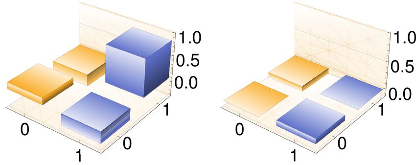
2

           a                                  b                                   c

Figure 1. Several hybrid (trusted-untrusted) multipartite scenarios. In the device-dependent (DD) case, measurement devices are well char-
acterized (trusted), so that a specific quantum state (represented by Bloch spheres) can be attributed to the system. In the device-independent
(DI) case, in contrast, the devices are uncharacterized (untrusted), so that systems are represented by black boxes. Semi-DI scenarios
contain both trusted and untrusted components. There, the joint system is mathematically described by a hybrid object – intermediate
between a state and a Bell behavior – called assemblage, and the type of nonlocality they can feature is called steering. In all three panels
the shaded plane illustrates the bipartition of the trusted subsystem versus the untrusted ones. a An assemblage in the 2DI+1DD scenario:
Alice and Bob rely on a black-box description, whereas Charlie’s system is trusted. All three subsystems are space-like separated. b Alice
and Bob are no longer space-like separated: she communicates her output to him and he uses this to choose his input. This is an example
of a bilocal wiring (local with respect to the bipartition AB|C). Such operations cannot create any correlations across the bipartition, but
they can expose a subtle form of multipartite quantum nonlocality that otherwise does not violate any Bell or steering inequality across the
bipartition (see text). c A 4DI+1DD assemblage is mapped onto a 2DI+1DD one by a bilocal wiring (x2 = a3 , x3 = x4 , and a01 = a1 + a2
mod 2). Such wirings can implement non-trivial resource-theoretic transformations, but not enough to enable a multi-black-box universal
steering bit, i.e. an N -partite assemblage from which all bipartite ones, e.g., can be reached (see Supplementary Notes E).

for its quantification, classification, and operational manip-            use the term bilocal to refer to being local with respect to the
ulation (see, e.g., [29–31]). Applied and fundamental inter-              AB|C bipartition. It stands to reason that operations within
est has motivated their formulation for entanglement [1] and              a given partition are free. However, a “wiring” between A
Bell nonlocality [27, 32–34], as well as for other relevant               and B (e.g. linking the output of one black box to the input
quantum properties [34–39]. Most important for our discus-                of another as in Fig. 1 b) is confined to AB but can map
sion is the resource theory of steering [40, 41]. The corner-             tripartite Bell behaviors that are local in the AB|C partition
stone of any resource theory is the set of its free operations.           (i.e. bilocal) into bipartite Bell behaviors that violate a Bell
These are unable to create the resource: they transform ev-               inequality across AB|C. The problem, however, lied in the
ery resourceless state into a resourceless state. As a concrete           definition of Bell nonlocality in multipartite scenarios used
example, free operations for quantum steering include, on                 previously [43].
the untrusted side, pre and post-processings of classical vari-              According to the traditional definition [43], Bell nonlocal-
ables of the black boxes and, on the trusted side, local quan-            ity across a system bipartition is incompatible with any LHV
tum operations and classical communication to the untrusted               model with respect to it. This includes so-called “fine-tuned”
parties. It can be shown [40] that these operations cannot                models [44] with hidden signaling. These are LHV models
create quantum steering out of unsteerable systems.                       where, for each value of the hidden variable, the subsystems
   A fully DI description is cast in terms of a Bell behav-               on each side of the bipartition communicate, but for which
ior, given by a conditional probability distribution of the out-          the statistical mixture over all values of the hidden variable
puts given the inputs. Bell locality implies that there exists            renders the observable correlations non-signaling. The prob-
a local-hidden-variable (LHV) model, in which correlations                lem is that the bilocal wiring can conflict with the hidden
are explained by a (hypothetical) classical common cause                  signaling in such models, giving rise to a causal loop. For
(the hidden variable) within the common past light-cone of                instance, assume that for a particular tripartite system, there
the measurement events [42]. Any Bell-inequality violation                is only one LHV decomposition, which uses hidden signal-
implies incompatibility with LHV models, i.e. Bell nonlo-                 ing from Bob to Alice. To physically implement the wiring
cality. Bell-local behaviors are, naturally, the resourceless             in Fig. 1b, which is an example of a free operation allowed
states of the resource theory of Bell nonlocality. We shall               within the AB partition, Bob must be in the causal future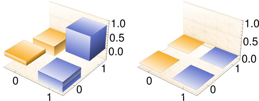
3

of Alice. This, in turn, is inconsistent with the direction of     behavior is not guaranteed to admit a physical realization,
the hidden signaling. This explains why apparently bilocal         i.e. it may be supra-quantum [50–52]. Therefore, we also
behaviors can lead to Bell violations after a bilocal wiring.      derive an alternative protocol that – albeit not universal – is
A redefinition of multipartite Bell nonlocality was then pro-      manifestly within quantum theory. Moreover, we show that
posed [27, 28]. This considers the correlations from conflict-     the output assemblage of such protocol is not only steerable
ing bilocal models as already nonlocal across the bipartition,     but also Bell nonlocal (in the sense of producing a nonlocal
so that the wiring simply exposes an already-existing subtle       behavior upon measurements by Charlie). This is notable
form of Bell nonlocality. We refer to the latter form and ef-      as Bell nonlocality is a stronger form of quantum correlation
fect as subtle Bell nonlocality and Bell-nonlocality exposure,     than steering. We refer to this effect as super-exposure of Bell
respectively.                                                      nonlocality. In turn, we provide a redefinition of (both mul-
    The redefinition fixed the inconsistency, but also opened      tipartite and genuinely multipartite) steering to re-establish
several intriguing questions. First, no experimental observa-      operational consistency. Finally, we experimentally demon-
tion of Bell-nonlocality exposure has been reported. Second,       strate exposure as well as super-exposure. This is done using
even though steering theory is relatively mature [22, 45–48],      polarization and path degrees of freedom of two entangled
little is known about steering exposure. Steering features         photons generated by spontaneous parametric down conver-
in the semi-DI description, where systems are described in         sion, in a deterministic protocol.
terms of assemblages, given by quantum states describing
the DD subsystems, weighted by the conditional probabili-
                                                                                         PRELIMINARIES
ties describing the DI parties. Operational consistency rel-
ative to steering exposure was considered, in particular, in
a definition of multipartite steering [22], but based on mod-                     Steering and the semi-DI setting
els where each party is probabilistically either trusted or un-
trusted. On the other hand, a definition based on multipar-            Most of our discussion will be based on the semi-DI set-
tite entanglement certification in semi-DI setups with fixed       ting of Fig. 1a. We will not resort to quantum models of the
trusted-versus-untrusted divisions was proposed in Ref. [49].      black boxes; our definitions are based on the semi-DI set-
There, bilocal hidden-variable models with an explicit quan-       ting alone, as befits its treatment as a resource for quantum
tum realization are considered, which automatically rules          tasks. Such systems are fully described by a Bell behav-
out potentially-conflicting fined-tuned models. Nevertheless,      ior P (AB) := {Pa,b|x,y }a,b,x,y , with Pa,b|x,y the conditional
this has the side-effect of over-restricting the set of unsteer-   probability of outputs a, b given inputs x, y, for Alice and
able assemblages, thus potentially over-estimating steering.       Bob, and an ensemble of conditional quantum states %a,b|x,y
Third, exposure as a resource-theoretic transformation is yet      for Charlie. These can be encapsulated in a hybrid object
unexplored territory. For instance, is it possible to obtain ev-   known as the assemblage σ := {σa,b|x,y }a,b,x,y , of sub-
ery bipartite assemblage via exposure from some multipartite       normalized conditional states σa,b|x,y := Pa,b|x,y %a,b|x,y .
one? What about Bell behaviors? Moreover, is there a sin-              Unlike in Bell nonlocality or entanglement, semi-DI sys-
gle N -partite assemblage from which all bipartite ones are        tems have a natural bipartition: the one separating the trusted
obtained via exposure?                                             devices from the untrusted ones, AB|C. This is the bipar-
    These are the questions we answer. To begin with, we           tition with respect to which we define steering throughout,
show that, remarkably, exposure of quantum nonlocality is a        unless otherwise explicitly stated. We assume that σ sat-
universal effect, in the sense that every bipartite Bell behav-    isfies the no-signaling (NS) principle, by virtue of which
ior (assemblage) can be the result of Bell-nonlocality (steer-     measurement-outcome correlations alone do not allow for
ing) exposure starting from some tripartite one. This high-        communication. This implies that the statistics observed by
lights the power of exposure as a resource-theoretic trans-        Charlie should be independent of the input(s) of the remain-
formation. However, we also delimit such power: we prove           ing user(s). Mathematically, this condition reads
a no-go theorem for multi-black-box universal steering bits:                       X
                                                                                       σa,b|x,y = %(C) , ∀ x, y,                (1)
there exists no single N -partite assemblage (with N − 1 un-
                                                                                   a,b
trusted and 1 trusted devices) from which all bipartite ones
                                                                           (C)
can be obtained through free operations of steering. Interest-     where %    is the reduced state on C. Furthermore, we also
ingly, in the universal steering exposure protocol, the starting   assume that Alice and Bob are NS, i.e. choosing their inputs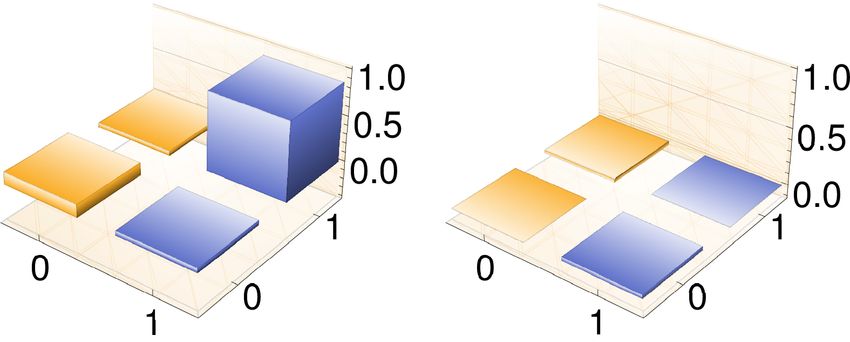
4

does not provide them any communication,                            producing any bipartite assemblage (behavior) whatsoever
          X                                                         from an appropriate tripartite assemblage (behavior) origi-
              σa,b|x,y independent of x, ∀ b, y,             (2)    nally admitting an LHS (LHV) model. As in Ref. [27], we
            a                                                       exploit bilocal wirings as that of Fig. 1b, which makes Bob’s
          X                                                         input y equal to Alice’s output a. This requires that Bob’s
                σa,b|x,y independent of y,     ∀ a, x.       (3)
                                                                    measurement is in the causal future of Alice’s. Indeed, after
            b
                                                                    the wiring, systems A and B now behave as a single black
  The definition of steering in the AB|C partition hinges on        box with input x and output b. In other words, exposure is a
the impossibility of decomposing an assemblage σ as                 form of conversion from tripartite correlations into bipartite
                                                                    ones. Here, we restrict to the case of binary inputs and out-
                                                                    puts (x, y, a, b ∈ {0, 1}) for simplicity, where we prove the
                         X
             σa,b|x,y =       Pλ Pa,b|x,y,λ %λ .         (4)
                           λ
                                                                    following surprising result.

Here, Pλ is the probability of the hidden variable Λ tak-           Theorem 1 (Universal exposure of quantum nonlocality).
                           (AB)                                     Any bipartite assemblage σ (target) or Bell behavior P (target)
ing the value λ, each P λ         := {Pa,b|x,y,λ }a,b,x,y is a λ-
                                                                    can be obtained via the wiring y = a on the tripartite assem-
dependent behavior, and %λ is the λ-th hidden state for C (lo-
cally correlated with AB only via Λ). However, different ap-        blage σ (initial) or behavior P (initial) , respectively, of elements
proaches have diverging positions on the set to which the dis-                                             1 (target)
             (AB)                                                                           (initial)
tribution P λ     may belong. Possibilities range [5] from the                            σa,b|x,y :=       σ                           (5)
                                                                                                           2 b|x⊕a⊕y
full set of valid bipartite distributions to the most restricted
set of factorizable ones (i.e. Pa,b|x,y,λ = Pa|x,λ Pb|y,λ           or
∀a, b, x, y). In [49], steering is treated as equivalent to en-                                         1 (target)
tanglement certification, hence each distribution P λ
                                                         (AB)
                                                               is    P (initial) (a, b, c|x, y, z) =      P        (b, c|x ⊕ a ⊕ y, z) , (6)
                                                                                                        2
required to be quantum-mechanically realizable. Our opera-
tional approach is defined in terms of assemblages only and         where ⊕ stands for addition modulo 2. Moreover, σ (initial)
aims to use them as resources, not for inferences on the quan-      and P (initial) admit respectively an LHS and an LHV models
tum models that can produce them. It is thus best to ignore         across the AB|C bipartition, for all σ (target) and P (target) .
restrictions and consider, as a starting point, a general prob-
ability distribution. As such, σ is unsteerable if it admits a         That the initial correlations are mapped to the desired tar-
local hidden-state (LHS) model, defined by Eq.(4) with gen-         get is self-evident from Eqs. (5,6). What is certainly not evi-
       (AB)
eral P λ ; otherwise σ is steerable.                                dent is that the initial correlations are bilocal. This is proven
   Importantly, a non-signaling σ does not imply non-               in Supplementary Notes A by construction of explicit LHS
              (AB)                                                  and LHV models. When the target assemblage (behavior)
signaling P λ      for each λ. (Imposition of the latter would
                                                                    is steerable (Bell nonlocal), exposure of steering (Bell non-
be an additional requirement, one that is used in [4] for yet
                                                                    locality) is achieved. Furthermore, apart from steerable, as-
another definition of steering in the literature.) In fact, LHS
                                                                    semblages can also be Bell nonlocal in the sense of giving
models can exploit hidden signaling between Alice and Bob
                                                                    rise to nonlocal behaviors under local measurements [47].
as long as communication at the observable level (i.e. upon
                                                                    Hence, when σ (target) is Bell nonlocal, a seemingly unsteer-
averaging Λ out) is impossible. This effect is known as fine-
                                                                    able system — i.e. one that admits an LHS decomposition
tuning [44] and will turn out to be critical.
                                                                    — is mapped onto a Bell nonlocal one, which is outstanding
                                                                    in view of the fact that unsteerable assemblages form a strict
                                                                    subset of Bell-local ones.
                           RESULTS
                                                                       The protocol highlights the capabilities of bilocal wirings
                                                                    as resource-theoretic transformations. Remarkably, such
    Steering exposure and Bell-nonlocality super-exposure           wirings compose a strict subset of well-known classes of free
                                                                    operations of quantum nonlocality (across AB|C): local op-
  We begin by an exposure protocol for steering and Bell            erations with classical communication (LOCCs) [1] for en-
nonlocality that is universal in the sense of being capable of      tanglement, one-way (1W) LOCCs from the trusted to the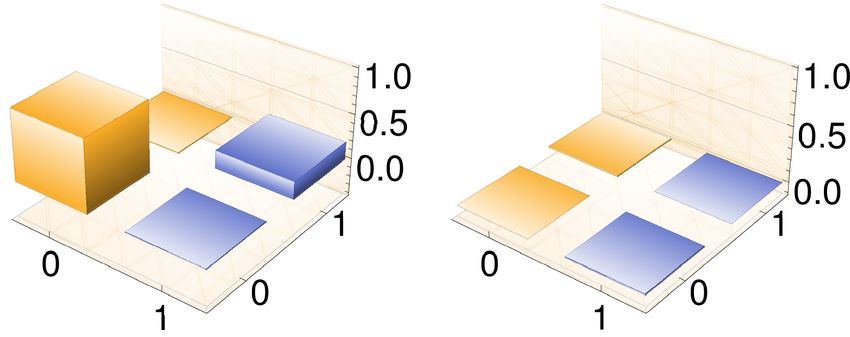
5

untrusted parts [40] for steering, and local operations with       composition and still be steerable. We describe this redefini-
shared randomness [27, 32, 33] for Bell nonlocality. How-          tion, analogous to the one in [27], before moving on to the
ever, there are also limitations to the capabilities of these      experimental realization.
wirings. In particular, in Supplementary Notes E we prove
a no-go theorem for universal steering bits in the N DI+1DD
scenario [exemplified in Fig. 1c for N = 4]. That is, we                               Consistently defining steering
show there that there is no N -partite assemblage, for all N ,
from which all bipartite ones can be obtained via arbitrary           The existence of subtle steering implies a stark inconsis-
1W-LOCCs.                                                          tency between the naive definition of steering from LHS de-
   Although the protocol above is universal, it is unclear         composability, Eq. (4), and the notion of locality. Since the
whether it can actually be physically implemented in general.      free operations that cause exposure are classical and strictly
This is due to the fact that the tripartite initial correlations   local (fully contained in the AB partition), it is reasonable
may be supra-quantum, i.e. well-defined non-signaling cor-         that they are unable to create not only steering but also any
relations that can however not be obtained from local mea-         form of correlations (even classical ones) across AB|C. The
surements on any quantum state [50–53]. Physical protocols         alternative left is to redefine bipartite steering in multipar-
for Bell-nonlocality exposure were devised in Refs. [27, 28],      tite scenarios such that, e.g., the assemblages in Eqs. (5) and
but no such protocols have been reported for steering. Hence,      (7) are already steerable. Formally, we need to exclude a
we next derive an alternative example for both steering expo-      subclass of LHS decompositions from the set of unsteerable
sure and Bell-nonlocality super-exposure that is manifestly        assemblages.
within quantum theory. This also exploits the bilocal wirings         To identify that subclass, let us apply the wiring y = a to
of Fig. 1b, but starting from a different initial assemblage.      a general σ fulfilling Eq. (4). This gives σ (wired) , of elements
We describe the latter directly in terms of its quantum re-                                               X
                                                                       (wired)
                                                                                  X              X
alization. Consider a tripartite
                               √ Greenberg-Horne-Zeilinger           σb|x      :=    σa,b|x,a =        Pλ       Pa,b|x,a,λ %λ . (9)
(GHZ) state (|000i + |111i)/ 2, with |0i and |1i the eigen-                        a                λ          a
vectors of the third Pauli matrix Z. Bob makes von Neumann
measurements on his share of the state for both his inputs,        This is a valid LHS decomposition as long as the term within
for y = 0 in the Z + X basis and for y = 1 in the Z − X            parentheses yields a valid (normalized) conditional probabil-
basis, with X the first Pauli matrix. Alice, however, makes        ity distribution (of B given X and Λ). This is the case if
                                                                             (AB)
either a trivial measurement, given by the positive operator-      every P λ       in Eq. (4) is non-signaling. In that case, by
valued measure {1/2, 1/2}, for x = 0, or a von Neumann             summing over b and applying the NS condition, one gets
X-basis measurement, for x = 1. For the resulting initial as-
semblage, σ (GHZ) , the following holds (see Supplementary                                               NS
                                                                       X                    X                 X
                                                                             Pa,b|x,a,λ =        Pa|x,a,λ =        Pa|x,λ = 1 ,   (10)
Notes B for more details).                                             a,b                   a                a

Theorem 2 (Physically-realizable exposure and super-expo-
sure). The quantum assemblage σ (GHZ) , of elements                which renders σ (wired) indeed unsteerable. However, this rea-
                                                                                                                   (AB)
                                                                   soning can in general not be applied if any P λ      is signal-
                      (−1)b

      (GHZ)    1                           a+y
                                                                  ing from Bob to Alice, i.e. if Alice’s marginal distribution
    σa,b|x,y =     1+ √       Z + x(−1)        X      (7)          for a depends on y (apart from x and λ). Therefore, we see
               8         2
                                                                   that the inconsistency is rooted at hidden signaling. In fact,
admits an LHS model and, under the wiring y = a, is                at the level of the underlying causal model, the phenomenon
mapped to the assemblage of elements                               of exposure can be understood as a causal loop between such
                                                                   signaling and the applied wiring (see Fig. 2).
                          (−1)b

                  1                                                   To restore consistency, hidden signaling must be re-
           σb|x =    1 + √ (Z + xX) ,           (8)
                  4           2                                    stricted. An obvious possibility would be to allow only for
                                                                                      (AB)
which is both steerable and Bell-nonlocal.                         non-signaling P λ ’s in Eq. (4). Interestingly, however,
                                                                   this turns out to be over-restrictive. Following the redefini-
   These results require a redefinition of steering in the mul-    tion of multipartite Bell nonlocality [27, 28], we propose the
tipartite scenario, since an assemblage can admit an LHS de-       following for bipartite steering in multipartite scenarios.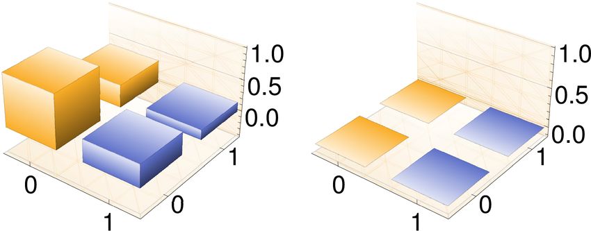
6

                                                                                         all NS assemblages
                                λ                                                        LHS

         x                      y                                                        TO-LHS
                        g
                    ri n
               wi                                                                        NS-LHS
                                                           ρ
         a                      b                                       Figure 3.       Pictorial representation of inner structure of the set
                                                                        of all non-signaling assemblages in the tripartite scenario. Inclu-
Figure 2. Steering exposure as a causal loop. In the causal net-        sion is strict for all depicted subsets: the set LHS of generic local-
work underlying LHS models, given by Eq. (4), the hidden variable       hidden-state (LHS) assemblages, the set TO-LHS of time-ordered
λ directly influences Charlie’s quantum state % as well as the Alice    LHS ones, the set NS-LHS of non-signaling LHS ones, and the
and Bob’s outputs a and b, which are in turn also influenced by the     set Q-LHS of quantum-LHS ones (see Supplementary Notes C for
inputs x and y, respectively. Even though the observed assemblage       details). The shaded region represents the set of assemblages with
(after averaging λ out) is non-signaling, the model can still exploit   subtle steering. Bilocal wirings can expose such steering by map-
hidden signaling (i.e. at the level of λ). For instance, for each λ,    ping that region to the set of (bipartite) steerable assemblages.
Alice’s output may depend (red arrow) on Bob’s input in a different
fine-tuned way such that the dependence vanishes at the observable
level. The wiring of Fig. 1b forces y = a, closing a causal loop that   sure is possible for TO-LHS assemblages, guaranteeing con-
will in general conflict with the latter dependence for some λ. As
                                                                        sistency with bilocal wirings (as well as generic 1W-LOCCs
a consequence, the final assemblage resulting from the wiring may
not admit a valid LHS decomposition, exposing steering. Hence,
                                                                        from trusted to untrusted parts) as free operations of steering.
the exposure can in a sense be thought of as an operational bench-      We note that, even though this redefinition prevents the ex-
mark for hidden signaling in the LHS model describing the initial       posure effect from creating steering, the effect still has, as il-
assemblage.                                                             lustrated by the exposure theorems, a relevant transformation
                                                                        power, especially when applied to steerable assemblages. As
                                                                        an example, there are assemblages that can only violate a
Definition 1 (Redefinition of steering). An assemblage σ is             Bell inequality across AB|C after the exposure protocol.
unsteerable if it admits time-ordered LHS (TO-LHS) decom-                  On the other hand, when all λ-dependent behaviors in Eqs.
positions both from A to B and from B to A simultaneously,              (11,12) are fully non-signaling, then the assemblage is called
i.e. if                                                                 non-signaling LHS (NS-LHS). There exists TO-LHS assem-
                                                                        blages that are not NS-LHS, which proves that the latter is
                                   (A→B)
                          X
              σa,b|x,y =      Pλ Pa,b|x,y,λ %λ         (11)             a strict subset of the former. In Supplementary Notes C,
                                λ                                       we provide a quantum and a supra-quantum example of TO-
                                          (B→A)                         LHS assemblages that are not NS-LHS.
                                X
                            =       Pλ0 Pa,b|x,y,λ %0λ ,        (12)
                                λ
                                                                           This definition based on TO-LHS models is strictly differ-
                                                                        ent from previous definitions of steering in the literature. In
                (A→B)                                                          (AB)
where each P λ      is non-signaling from Bob to Alice and              [4], P λ     from Eq.(4) is restricted to non-signaling distri-
       (B→A)
each P λ      from Alice to Bob. Otherwise σ is steerable.              butions, which coincides with the NS-LHS definition. In [49]
                                                                           (AB)
                                                                        Pλ       is further restricted to quantum-realizable bipartite
   The validity of both time orderings simultaneously pre-              distributions, in what constitutes the quantum-LHS model,
vents conflicting causal loops. More precisely, if a wiring             see Fig. 3. A fully factorizable P λ
                                                                                                            (AB)
                                                                                                                  , as mentioned in [5],
from Alice to Bob is applied on σ, one uses decompo-                    represents an even further restriction, and the corresponding
                                 (A→B)
sition (11) to argue with the P λ       ’s [as in Eq. (10)]             model only allows for classical correlations between Alice,
that the wired assemblage is unsteerable. Analogously, if               Bob, and Charlie.
a wiring from Bob to Alice is performed, one argues using                  These examples have another consequence for the defi-
       (B→A)
the P λ      ’s from decomposition (12). Hence, no expo-                nition of steering. At times has the definition of steering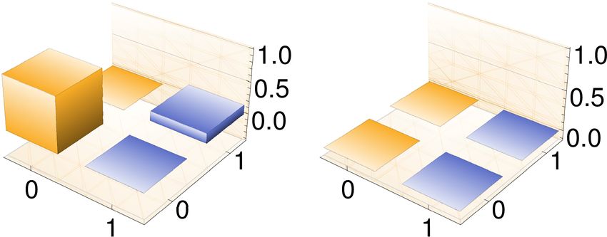
7

been stated as entanglement that can be certified with the                                                              Charlie
reduced information content of a semi-DI setting [19, 49].
In fact, even with steering defined independently of entan-                    i           Alice                               D1
                                                                                           0            PBSA                        &
glement certification, never to our knowledge had there been             BBO   s
an instance of one being present without the other. We have                                        Δ                           D2
                                                                                           1           H@θ     H@45°
nevertheless found cases of entanglement certification in the
                                                                    GHZ preparation
semi-DI scenario without steering, dissociating these two no-                                                                  D3
tions: the latter is sufficient, but not necessary, for the for-                                                                    Bob
mer. This is seen from the quantum-realizable examples of
a TO-LHS assemblage that is not NS-LHS in Supplemen-                               Δ   =
                                                                                                       BD      H    Q    PBS
tary Notes C. They can be decomposed as in Eqs. (11,12),
                                 (A,B→B,A)
but only with distributions Pa,b|x,y,λ       that are signaling,
                                                                   Figure 4. Experimental setup. Two crossed-axis BBO crystals are
hence, not quantum. As such, a quantum system without
                                                                   pumped by a He-Cd laser centered at 325 nm, producing pairs of
AB|C entanglement is unable to produce such an assem-              photons at 650 nm entangled in the polarization degree of freedom
blage, i.e. entanglement can be certified in AB|C. On the          [54]. The signal (s) photon is sent through a BD which deviates
other hand, since it is TO-LHS, the assemblage has no steer-       only the horizontal-polarization component, producing a tripartite
ing in the same bipartition (details in Supplementary Notes        GHZ state on two photons using polarization and path degrees of
C).                                                                freedom. Idler (i) photons are sent directly to Charlie’s polarization
   Furthermore, the redefinition above automatically implies       measurements. Signal photons are first measured in polarization by
also a redefinition of genuinely multipartite steering (GMS).      Alice, then Bob maps his path qubit onto a polarization qubit for his
We present this explicitly in Supplementary Notes D. There,        measurements. H stands for half-wave plate, Q for quarter-wave
we follow the approach of Ref. [49] in that a fixed trusted-       plate and P BS for polarizing beam splitter.
versus-untrusted partition is kept. However, instead of defin-
ing GMS as incompatibility with quantum-LHS assemblages
(i.e. with λ-dependent behaviors with explicit quantum real-       tomography are performed as described below.
izations) as in [49], we use the more general TO-LHS ones.            To implement the wiring from Fig. 1b, Alice’s polarization
This reduces the set of genuinely multipartite steerable as-       measurements are realized before Bob’s measurements onto
semblages safely, i.e. without introducing room for exposure.      the path degree of freedom. Alice’s results are read from the
The dissociation of steering and entanglement certification        output of PBSA , which determines whether D2 (a = 0) or
also happens in this genuine multipartite case.                    D3 (a = 1) clicks. For Alice’s trivial measurement (x = 0),
                                                                   crucial for the original assemblage to be LHS-decomposable,
                                                                   both her wave plates located before the imbalanced interfer-
                Experimental implementation                        ometer (represented by ∆) are kept at 0◦ , and H@θ is ad-
                                                                   justed to 22.5◦ . The role of ∆ is to remove the coherence
   The exposure procedure was experimentally implemented           between horizontal and vertical polarization components, en-
using entangled photons produced via spontaneous paramet-          suring that the photon exits PBSA randomly, independent of
ric down conversion. The experimental setup is shown in            the input polarization state. For x = 1, Alice’s wave plates
                                                          +
Fig. 4. A photon√ pair is generated in the Bell state |Φ i =       are set to project the polarization on the X eigenstates, the
(|00i + |11i) / 2, where |0i (|1i) stands for horizontal (ver-     interferometer and H@θ (θ = 0◦ ) play no role. Bob performs
tical) polarization of the photons [54]. The photons in the        his projective measurements by first mapping the path de-
signal mode (s) pass through a calcite beam displacer (BD),        grees of freedom onto polarization using BDs and then pro-
which creates two momentum modes (paths) depending on              jecting the polarization state using his set of wave plates and
the polarization. This results in a tripartite GHZ state, where    PBSs, as was realized in Ref. [55]. To reconstruct the as-
the extra qubit is the path degree of freedom of the photons       semblage in Eq. (7), measurements for y = 0 and y = 1 are
in s. Alice’s and Bob’s qubits are the polarization and path       made in both detectors D2 and D3 , varying the angle of the
of the photons in mode s, respectively, while Charlie’s qubit      wave plates in Bob’s box. To collect the data corresponding
is the polarization of the photons in mode i. Projective mea-      to the wired assemblage (8) only the y = 0 measurement is
surements onto all the degrees of freedom required for state       made in D2 (a = 0) and only y = 1 is made in D3 (a = 1),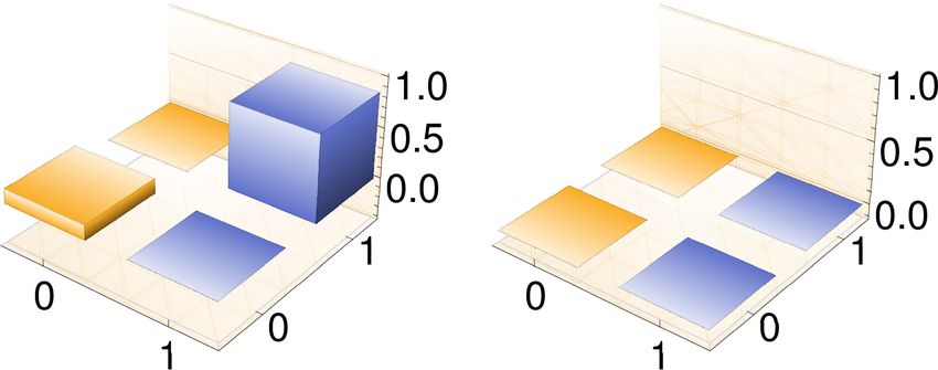
8

enforcing that Bob’s input equals Alice’s output (y = a).          a
   The assemblage σ (GHZ) was obtained experimentally by
performing state tomography on Charlie’s system for each
measurement setting and outcome of Alice and Bob. Six-
teen density matrices (plotted in Figure 7, in Supplementary
Material) are obtained through maximum likelihood, and the
assemblage presents a fidelity-like measure of 98.2 ± 0.2%
compared to the theoretical one (see Methods). The experi-
mental wired assemblage is shown in Fig. 5a, and returns a
fidelity of 98.1 ± 0.6% with respect to the theoretical wired      b
assemblage given in (8).
   An exact LHS decomposition of the experimental assem-
blage is not feasible due to imperfections and finite statistics
— in fact, assemblages reproducing raw experimental data
exactly are not even physical, since they disobey the NS prin-
ciple [49]. To show that the experimental tripartite assem-
blage is statistically compatible with an LHS decomposition,
we proceed as follows: First, we assume the photocounts
obtained for each measured projector are averages of Pois-         c
son distributions; with a Monte Carlo simulation, we sample
many times each of these distributions and reconstruct the
corresponding assemblages. Second, for each reconstructed
assemblage, we find the physical (NS) assemblage that best
approximates it through maximum-likelihood estimation, as
well as the best LHS approximation for comparison. As
an initial indication of LHS-compatibility, the log-likelihood
error of both approximations is extremely similar, see Fig.
5c. Third, for the NS approximations we calculate the LHS-         d
robustness [56], a measure which is zero for all LHS assem-
blages. For comparison, we repeat the procedure starting
with simulated finite-photocount statistics from the theoreti-
cal LHS assemblage from Eq. (7). In Fig. 5d we see that the
experimental robustness has a sizable zero component and a
distribution fully compatible with that of an LHS assemblage
under finite measurement statistics.
   To show that the experimental wired assemblage is steer-
able, we tested it on the optimal steering witness W with re-
spect to assemblage (8) (see Supplementary Notes B). This
returned a value 1.015 ± 0.009       1 (theoretical: 1.0721        Figure 5. Experimental results. a, b Experimental assemblages af-
                                                                   ter y = a wiring. a Real part of Charlie’s conditional density matri-
1), where the inequality violation implies steering, see Fig.
                                                                   ces, theoretical (top) and experimental (bottom). b Steering-witness
5b. This allows us to conclude that the bipartite wired as-        histogram. The witness value is 1.015 ± 0.009, meaning that the
semblage is indeed steerable. The experimental error was           experimental assemblage is more than one standard deviation above
calculated using 500 assemblages also from a Monte Carlo           the steering threshold (dashed line). c, d Compatibility of the tri-
simulation of measurement results with Poisson photocount          partite experimental assemblage with the naive (LHS) definition of
statistics.                                                        unsteerability [Eq. (4)]. c Histogram of the error of approximating
   Using the same experimental setup, we can also experi-          the tripartite assemblage by an NS and an LHS assemblage, show-
mentally demonstrate super-exposure of Bell nonlocality. As        ing that the error of assuming the LHS decomposition is as small
argued above, the initial experimental assemblage is compat-       as that of the physically necessary NS assumption. d From the best
                                                                   NS approximation to the experimental data, histogram of the LHS-
                                                                   robustness, a measure of deviations from the set LHS. Even with
                                                                   all experimental error, there is only a residual amount of robust-
                                                                   ness, fully compatible with that of the theoretical LHS assemblage
                                                                   solely under finite-statistics error. All histograms come from Monte
                                                                   Carlo simulation assuming Poisson distributions.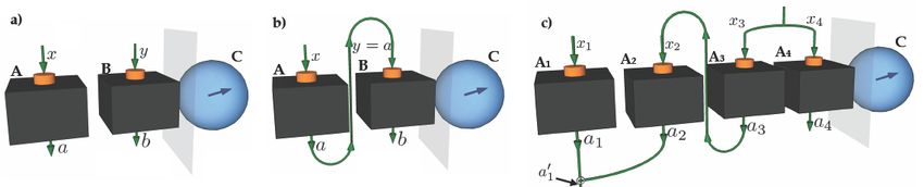
9

ible with an LHS model. Therefore, no matter what measure-         partite steering in multipartite scenarios and genuinely mul-
ment Charlie makes, the corresponding Bell behavior will           tipartite steering that does not leave room for creating cor-
be compatible with an LHV model. Hence, we must only               relations from scratch. Finally, both steering exposure and
show that the experimental wired assemblage is Bell non-           Bell nonlocality super-exposure have been demonstrated ex-
local. In Ref. [47], a necessary and sufficient criterion for      perimentally using an optical implementation. This is to our
Bell nonlocality of assemblages was derived: Given Alice           knowledge the first experimental observation of exposure
and Bob’s wired measurements (y = a) with input bit x and          of quantum nonlocality reported, not only in semi device-
output bit b, to maximally violate a Bell inequality, Charlie      independent scenarios but also in fully device-independent
performs von Neumann measurements in the 2Z + X and X              ones, as originally predicted in [27, 28].
bases, labeled by input bit z, obtaining binary output result c.      Finally, we mention practical implications that our results
They thus obtain sixteen probabilities P (b, c|x, z), which are    might have. Steering in the scenario we work on, with a
used to calculate the Clauser-Horne-Shimony-Holt (CHSH)            single trusted party, has been shown to be particularly rele-
inequality [57]. We obtained an experimental violation of          vant for the task of quantum secret sharing [24, 25]. In it,
2.21 ± 0.04 2 (theoretical prediction: 2.29 2), showing            the trusted party deals a secret to the untrusted parties, who
Bell nonlocality.                                                  must be able to access it only when cooperating, not inde-
   This experiment is sufficient to for a proof-of-principle       pendently. A form of steering that is only observable when
demonstration of both exposure of steering and super-              such parties cooperate, as in the exposure protocol, fits this
exposure of Bell nonlocality. We note that strict demonstra-       mold quite specifically. This indicates a potential application
tion of these phenomena in their appropriate DI scenarios          of our results, possibly in conjunction with the open question
requires a realization with space-like separation between the      of other joint operations able to achieve exposure.
parties (locality loophole), as well high-efficiency source and
detectors (fair-sampling assumption).
                                                                                            METHODS

                        DISCUSSION                                                   Experimental Assemblages

   We have demonstrated that the traditional definition of            Let us describe the quantum state and the assemblages
multipartite steering for more than one untrusted party based      produced in our experiment in more detail. Although we
on decomposability in terms of generic bilocal hidden-state        treat two of the qubits as black boxes, in order to ensure that
models presents inconsistencies with a widely accepted, ba-        the resulting assemblage is coming up from quantum mea-
sic notion of locality. We have also shown how, according to       surements performed onto a GHZ, we first made a state to-
such definition, a broad set of steerable (exposure) and even      mography to determine the tripartite quantum state. This can
Bell-nonlocal (super-exposure) assemblages would be cre-           be done without adding any optical element to the setup. By
ated from scratch, e.g. by bilocal wirings acting on a seem-       varying the angles on Alice’s quarter-wave plate and half-
ingly unsteerable assemblage, i.e. an LHS one. A surpris-          wave plate before the imbalanced interferometer, we set her
ing discovery that we have made is the fact that exposure of       apparatus to make any tomographic measurement in polar-
quantum nonlocality is a universal effect, in the sense that all   ization if we set H@θ to 0◦ . The tomographic projections for
steering assemblages as well as Bell behaviors can be ob-          the path degree of freedom of photons in s and polarization
tained as the result of an exposure protocol starting from         of photons in i is done using the set of wave plates just before
bilocal correlations in a scenario with one more untrusted         detectors D1 and D2 , respectively. Using the collected coin-
party. This highlights the power of exposure as a resource-        cidence counts we reconstructed the tripartite quantum state
theoretic transformation. However, we also delimit such            by maximum likelihood. The reconstructed density matrix is
power: we prove a no-go theorem for multi-black-box uni-           shown on Figure 6. The experimental state presents fidelity
versal steering bits: there exists no single assemblage with       with GHZ state equals to 0.981 ± 0.004.
many untrusted and one trusted party from which all assem-            Each element of the tripartite assemblage is composed of
blages with one untrusted and one trusted party can be ob-         Charlie’s conditional quantum state and the conditional prob-
tained through generic free operations of steering. To restore     ability Pa,b|x,y for the black boxes. All sixteen experimen-
operational consistency, we offer a redefinition of both bi-       tal Charlie’s density matrices are shown in Figure 7 (Sup-
10
fidelity can be seen as a mean of the fidelities of the quantum
Re ρ 0.4 Im ρ 0.4
parts weighted by the square root of blackbox probabilities.
It has the property of being 1 if all elements of the two
0.2 0.2 assemblages are equal and vanishes if all quantum states are
0.0 0.0 orthogonal.
1 1
1 11 1 11
1 10
110
0 1 10 00 01
00 001 0 10001
100
0 10001
0 0 10 1 0
0 11
01 011 0 0 11 0 01 0 DATA AND CODE AVAILABILITY
10 101 0 00110
001
10 101 0 00110
0 0 0 0
11 111 0 11 111 0
The datasets and programming codes generated and/or an-
Figure 6. Real and imaginary parts of the experimental recon- alyzed during the current study are available from the corre-
structed GHZ state. Colors are for visualization purposes only. sponding author on reasonable request.
plementary Material) in comparison with the corresponding ACKNOWLEDGMENTS
theoretical ones. The associated conditional probabilities are
also shown. We thank Elie Wolfe and an anonymous referee for
For the wired assemblage, the expected conditional prob- independently pointing out a mistake in an earlier ver-
ability of each outcome is 12 ; the experimental values are sion of our manuscript. The authors acknowledge finan-
0.46 ± 0.01, 0.54 ± 0.01, 0.49 ± 0.01, 0.51 ± 0.01 (fol- cial support from the Brazilian agencies CNPq (PQ grants
lowing the order in Fig. 5a). The imaginary components of 311416/2015-2, 304196/2018-5 and INCT-IQ), FAPERJ
the density matrix average to 0.05 ± 0.02 (theoretical: zero). (PDR10 E-26/202.802/2016, JCN E-26/202.701/2018, E-
26/010.002997/2014, E-26/202.7890/2017), CAPES (PRO-
CAD2013), and the Serrapilheira Institute (grant number
Serra-1709-17173). SPW received support from Fondo
Assemblage Fidelity Nacional de Desarrollo Cientı́fico y Tecnológico (ANID)
(1200266) and ANID – Millennium Science Initiative Pro-
We can see by visual inspection that the experimental gram – ICN17 012.
and corresponding theoretical assemblage elements shown
in Figs. 5 and 7 (Supplementary Material) are similar. To
quantify this similarity we use a mean assemblage fidelity COMPETING INTERESTS
between two assemblages σ 1 = {P1 (a|x)%1 (a|x)} and
σ 2 = {P2 (a|x)%2 (a|x)} defined by The authors declare no competing interests.
F (σ 1 , σ 2 ) =
AUTHOR CONTRIBUTIONS
1 Xp
P1 (a|x)P2 (a|x)F (%1 (a|x), %2 (a|x)) , (13)
Nx x,a The theorems were derived by MMT (analytical) and RVN
(codes). MMT and LA performed the causal analysis, and
where x (a) is a list of inputs (outputs) of all black boxes, wrote most of the manuscript, with contributions from all au-
Nx is the number of different measurement choices, and thors. GHA and SPW have designed the experiment, which
F(%1 , %2 ) is the usual fidelity between two quantum states. was performed by TLS and GHA. TLS and RVN analyzed
The numerical values of assemblage fidelity in the main the results. SPW and LA conceived the original idea of ex-
text are calculated with this definition. The above defined ploring wirings as a resource.
[1] Ryszard Horodecki, Paweł Horodecki, Michał Horodecki, Phys. 81, 865–942 (2009), arXiv:quant-ph/0702225.
and Karol Horodecki, “Quantum entanglement,” Rev. Mod.11
[2] Nicolas Brunner, Daniel Cavalcanti, Stefano Pironio, Valerio A Review,” Adv. Quantum Technol. 3, 2000025 (2020),
Scarani, and Stephanie Wehner, “Bell nonlocality,” Rev. Mod. arXiv:2003.10186.
Phys. 86, 419–478 (2014), arXiv:1303.2849. [19] H. M. Wiseman, S. J. Jones, and A. C. Doherty, “Steering,
[3] M. D. Reid et al, “Colloquium : The Einstein-Podolsky-Rosen Entanglement, Nonlocality, and the EPR Paradox,” Phys. Rev.
paradox: From concepts to applications,” Rev. Mod. Phys. 81, Lett. 98, 140402 (2006), arXiv:quant-ph/0612147 .
1727–1751 (2009), arXiv:0806.0270. [20] S. J. Jones, H. M. Wiseman, and A. C. Doherty, “En-
[4] D. Cavalcanti and P. Skrzypczyk, “Quantum steering: a review tanglement, Einstein-Podolsky-Rosen correlations, Bell non-
with focus on semidefinite programming,” Rep. Prog. Phys. locality, and steering,” Phys. Rev. A 76, 052116 (2007),
80, 024001 (2017), arXiv:1604.00501. arXiv:0709.0390v2.
[5] Roope Uola, Ana C. S. Costa, H. Chau Nguyen, and Otfried [21] Cyril Branciard, Eric G. Cavalcanti, Stephen P. Walborn, Va-
Gühne, “Quantum Steering,” Rev. Mod. Phys. 92, 015001 lerio Scarani, and Howard M. Wiseman, “One-sided device-
(2020), arXiv:1903.06663. independent quantum key distribution: Security, feasibility,
[6] Jonathan Barrett, Lucien Hardy, and Adrian Kent, “No Sig- and the connection with steering,” Phys. Rev. A 85, 010301
naling and Quantum Key Distribution,” Phys. Rev. Lett. 95, (2012), arXiv:1109.1435.
010503 (2005), arXiv:quant-ph/0405101. [22] Q. Y. He and M. D. Reid, “Genuine Multipartite Einstein-
[7] Antonio Acı́n, Nicolas Gisin, and Lluis Masanes, “From Bell’s Podolsky-Rosen Steering,” Phys. Rev. Lett. 111, 250403
Theorem to Secure Quantum Key Distribution,” Phys. Rev. (2013), arXiv:1212.2270.
Lett. 97, 120405 (2006), arXiv:quant-ph/0510094. [23] Paul Skrzypczyk and Daniel Cavalcanti, “Maximal Ran-
[8] Antonio Acı́n, Serge Massar, and Stefano Pironio, “Effi- domness Generation from Steering Inequality Violations
cient quantum key distribution secure against no-signalling Using Qudits,” Phys. Rev. Lett. 120, 260401 (2018),
eavesdroppers,” New J. Phys. 8, 126 (2006), arXiv:quant- arXiv:1803.05199.
ph/0605246. [24] Ioannis Kogias, Yu Xiang, Qiongyi He, and Gerardo Adesso,
[9] Antonio Acı́n et al, “Device-Independent Security of Quan- “Unconditional security of entanglement-based continuous-
tum Cryptography against Collective Attacks,” Phys. Rev. variable quantum secret sharing,” Phys. Rev. A 95, 012315
Lett. 98, 230501 (2007), arXiv:quant-ph/0702152 . (2017), arXiv:1603.03224.
[10] Roger Colbeck, Quantum And Relativistic Protocols For Se- [25] Yu Xiang, Ioannis Kogias, Gerardo Adesso, and Qiongyi
cure Multi-Party Computation, Ph.D. thesis, University of He, “Multipartite Gaussian steering: Monogamy constraints
Cambridge (2006), arXiv:0911.3814. and quantum cryptography applications,” Phys. Rev. A 95,
[11] Roger Colbeck and Adrian Kent, “Private randomness expan- 010101(R) (2017), arXiv:1603.08173.
sion with untrusted devices,” J. Phys. A Math. Theor. 44, [26] Chien-Ying Huang, Neill Lambert, Che-Ming Li, Yen-Te Lu,
095305 (2011), arXiv:1011.4474. and Franco Nori, “Securing quantum networking tasks with
[12] S. Pironio et al, “Random numbers certified by Bell’s theo- multipartite Einstein-Podolsky-Rosen steering,” Phys. Rev. A
rem,” Nature 464, 1021–1024 (2010), arXiv:0911.3427. 99, 012302 (2019), arXiv:1812.03251.
[13] Antonio Acı́n and Lluis Masanes, “Certified random- [27] Rodrigo Gallego, Lars Erik Würflinger, Antonio Acı́n, and
ness in quantum physics,” Nature 540, 213–219 (2016), Miguel Navascués, “Operational Framework for Nonlocality,”
arXiv:1708.00265. Phys. Rev. Lett. 109, 070401 (2012), arXiv:1112.2647.
[14] Alexandru Gheorghiu, Elham Kashefi, and Petros Wallden, [28] Jean-Daniel Bancal, Jonathan Barrett, Nicolas Gisin, and Ste-
“Robustness and device independence of verifiable blind fano Pironio, “Definitions of multipartite nonlocality,” Phys.
quantum computing,” New J. Phys. 17, 083040 (2015), Rev. A 88, 14102 (2013), arXiv:1112.2626.
arXiv:1502.02571. [29] Fernando G. S. L. Brandão and Gilad Gour, “Reversible
[15] Michal Hajdušek, Carlos A. Pérez-Delgado, and Joseph F. Framework for Quantum Resource Theories,” Phys. Rev. Lett.
Fitzsimons, “Device-Independent Verifiable Blind Quantum 115, 70503 (2015), arXiv:1502.03149.
Computation.” Preprint at http://arxiv.org/abs/1502.02563 [30] Fernando G. S. L. Brandão and Gilad Gour, “Erratum: Re-
(2015). versible Framework for Quantum Resource Theories [Phys.
[16] Jérémy Ribeiro, Gláucia Murta, and Stephanie Wehner, “Fully Rev. Lett. 115 , 070503 (2015)],” Phys. Rev. Lett. 115,
device-independent conference key agreement,” Phys. Rev. A 199901(E) (2015).
97, 022307 (2018), arXiv:1708.00798. [31] Bob Coecke, Tobias Fritz, and Robert W. Spekkens, “A
[17] Timo Holz, Hermann Kampermann, and Dagmar Bruß, “Gen- mathematical theory of resources,” Inf. Comput. 250, 59–86
uine multipartite Bell inequality for device-independent con- (2016), arXiv:1409.5531.
ference key agreement,” Phys. Rev. Res. 2, 023251 (2020), [32] Julio I de Vicente, “On nonlocality as a resource theory and
arXiv:1910.11360. nonlocality measures,” J. Phys. A Math. Theor. 47, 424017
[18] Gláucia Murta, Federico Grasselli, Hermann Kampermann, (2014), arXiv:1401.6941.
and Dagmar Bruß, “Quantum Conference Key Agreement:12
[33] Rodrigo Gallego and Leandro Aolita, “Nonlocality free [50] Ana Belén Sainz, Nicolas Brunner, Daniel Cavalcanti, Paul
wirings and the distinguishability between Bell boxes,” Phys. Skrzypczyk, and Tamás Vértesi, “Postquantum Steering,”
Rev. A 95, 032118 (2017), arXiv:1611.06932. Phys. Rev. Lett. 115, 190403 (2015), arXiv:1505.01430.
[34] Elie Wolfe, David Schmid, Ana Belén Sainz, Ravi Kunjwal, [51] A. B. Sainz, L. Aolita, M. Piani, M. J. Hoban, and
and Robert W. Spekkens, “Quantifying Bell: the Resource P. Skrzypczyk, “A formalism for steering with local quan-
Theory of Nonclassicality of Common-Cause Boxes,” Quan- tum measurements,” New J. Phys. 20, 083040 (2018),
tum 4, 280 (2020), arXiv:1903.06311. arXiv:1708.00756.
[35] Andreas Winter and Dong Yang, “Operational Resource The- [52] Ana Belén Sainz, Matty J. Hoban, Paul Skrzypczyk, and
ory of Coherence,” Phys. Rev. Lett. 116, 120404 (2016), Leandro Aolita, “Bipartite Postquantum Steering in Gen-
arXiv:1506.07975. eralized Scenarios,” Phys. Rev. Lett. 125, 050404 (2020),
[36] Eric Chitambar and Gilad Gour, “Critical Examination of In- arXiv:1907.03705.
coherent Operations and a Physically Consistent Resource [53] Sandu Popescu and Daniel Rohrlich, “Quantum nonlocality
Theory of Quantum Coherence,” Phys. Rev. Lett. 117, 030401 as an axiom,” Found. Phys. 24, 379–385 (1994), arXiv:quant-
(2016), arXiv:1602.06969. ph/9508009.
[37] A. Grudka et al, “Quantifying Contextuality,” Phys. Rev. Lett. [54] Paul G. Kwiat, Edo Waks, Andrew G. White, Ian Appelbaum,
112, 120401 (2014), arXiv:1209.3745. and Philippe H. Eberhard, “Ultrabright source of polarization-
[38] Barbara Amaral, Adán Cabello, Marcelo Terra Cunha, and Le- entangled photons,” Phys. Rev. A 60, R773–R776 (1999),
andro Aolita, “Noncontextual Wirings,” Phys. Rev. Lett. 120, arXiv:quant-ph/9810003 .
130403 (2018), arXiv:1705.07911. [55] O. Jiménez Farı́as et al, “Observation of the Emergence of
[39] Márcio M. Taddei, Ranieri V. Nery, and Leandro Aolita, Multipartite Entanglement Between a Bipartite System and its
“Quantum superpositions of causal orders as an operational re- Environment,” Phys. Rev. Lett. 109, 150403 (2012).
source,” Phys. Rev. Res. 1, 033174 (2019), arXiv:1903.06180. [56] Ana Belén Sainz, Leandro Aolita, Nicolas Brunner, Rodrigo
[40] Rodrigo Gallego and Leandro Aolita, “Resource Theory of Gallego, and Paul Skrzypczyk, “Classical communication
Steering,” Phys. Rev. X 5, 041008 (2015), arXiv:1409.5804. cost of quantum steering,” Phys. Rev. A 94, 012308 (2016),
[41] Eneet Kaur and Mark M. Wilde, “Relative entropy of steering: arXiv:1603.05079.
on its definition and properties,” J. Phys. A Math. Theor. 50, [57] John F. Clauser, Michael A. Horne, Abner Shimony, and
465301 (2017), arXiv:1612.07152. Richard A. Holt, “Proposed Experiment to Test Local Hidden-
[42] John S. Bell, “On the Einstein Podolsky Rosen paradox,” Variable Theories,” Phys. Rev. Lett. 23, 880–884 (1969).
Phys. Phys. Fiz. 1, 195–200 (1964). [58] Rodrigo Gallego, Lars Erik Würflinger, Antonio Acı́n, and
[43] George Svetlichny, “Distinguishing three-body from two- Miguel Navascués, “Quantum Correlations Require Multipar-
body nonseparability by a Bell-type inequality,” Phys. Rev. D tite Information Principles,” Phys. Rev. Lett. 107, 210403
35, 3066–3069 (1987). (2011), arXiv:1107.3738.
[44] Christopher J. Wood and Robert W. Spekkens, “The lesson of [59] Marie-Christine Roehsner, Joshua A. Kettlewell, Tiago B.
causal discovery algorithms for quantum correlations: causal Batalhão, Joseph F. Fitzsimons, and Philip Walther, “Quantum
explanations of Bell-inequality violations require fine-tuning,” advantage for probabilistic one-time programs,” Nat. Com-
New J. Phys. 17, 033002 (2015), arXiv:1208.4119. mun. 9, 5225 (2018), arXiv:1709.09724.
[45] E. G. Cavalcanti, Q. Y. He, M. D. Reid, and H. M. Wiseman,
“Unified criteria for multipartite quantum nonlocality,” Phys.
Rev. A 84, 032115 (2011), arXiv:1008.5014.
[46] Seiji Armstrong et al, “Multipartite Einstein–Podolsky–Rosen
steering and genuine tripartite entanglement with optical net-
works,” Nat. Phys. 11, 167–172 (2015), arXiv:1412.7212.
[47] M. M. Taddei, R. V. Nery, and L. Aolita, “Necessary and
sufficient conditions for multipartite Bell violations with
only one trusted device,” Phys. Rev. A 94, 032106 (2016),
arXiv:1603.05247.
[48] Che-Ming Li et al, “Genuine High-Order Einstein-Podolsky-
Rosen Steering,” Phys. Rev. Lett. 115, 010402 (2015),
arXiv:1501.01452.
[49] D. Cavalcanti et al, “Detection of entanglement in asymmet-
ric quantum networks and multipartite quantum steering,” Nat.
Commun. 6, 7941 (2015), arXiv:1412.7730.Supplemental Material to:
Exposure of multipartite quantum nonlocality
M. M. Taddei,1, 2, ∗ T. L. Silva,1 R. V. Nery,1, 3 G. H. Aguilar,1 S. P. Walborn,1, 4, 5 and L. Aolita1, 6
1
Federal University of Rio de Janeiro, Caixa Postal 68528, Rio de Janeiro, RJ 21941-972, Brazil
2
ICFO - Institut de Ciencies Fotòniques, The Barcelona Institute of Science and Technology, 08860, Castelldefels, Barcelona, Spain
3
International Institute of Physics, Federal University of Rio Grande do Norte, 59070-405, Natal, Brazil
4
Departamento de Fı́sica, Universidad de Concepción, 160-C Concepción, Chile
5
ANID – Millennium Science Initiative Program – Millennium Institute for Research in Optics,
Universidad de Concepción, 160-C Concepción, Chile
6
Quantum Research Centre, Technology Innovation Institute, Abu Dhabi, UAE
(Dated: March 17, 2021)
This Supplementary Material is composed of Figure 7 and Supplementary Notes, divided into Sections A through E. Cita-
tions refer to the list of references of the main paper.
∗ marciotaddei@gmail.com14
a=0 b=0 a=0 b=1 a=1 b=0 a=1 b=1
P0,0|0,0=0.225±0.009 P0,1|0,0=0.27±0.01 P1,0|0,0=0.237±0.009 P1,1|0,0=0.27±0.01
1.0 1.0 1.0 1.0 1.0 1.0 1.0 1.0
0.5 0.5 0.5 0.5 0.5 0.5 0.5 0.5
x=0 y=0
0.0 0.0 0.0 0.0
0.0 0.0 0.0 0.0
1 1 1 1 1 1 1 1
0 0 0 0 0 0 0 0
0 0 0 0 0 0 0 0
1 1 1 1
1.0 1.0 1.0 1.0 1.0 1.0 1.0 1.0
0.5 0.5 0.5 0.5 0.5 0.5 0.5 0.5
0.0 0.0 0.0 0.0 0.0 0.0 0.0 0.0
1 1 1 1 1 1 1 1
0 0 0 0 0 0 0 0
0 0 0 0 0 0 0 0
1 1 1 1 1 1 1 1
P0,0|0,1=0.220±0.009 P0,1|0,1=0.28±0.01 P1,0|0,1=0.231±0.009 P1,1|0,1=0.269±0.009
1.0 1.0 1.0 1.0 1.0 1.0 1.0 1.0
0.5 0.5 0.5 0.5 0.5 0.5 0.5 0.5
0.0 0.0 0.0 0.0
x=0 y=1
0.0 0.0 0.0 0.0
1 1 1 1 1 1 1 1
0 0 0 0 0 0 0 0
0 0 0 0 0 0 0 0
1 1 1 1
1.0 1.0 1.0 1.0 1.0 1.0 1.0 1.0
0.5 0.5 0.5 0.5 0.5 0.5 0.5 0.5
0.0 0.0 0.0 0.0 0.0 0.0 0.0 0.0
1 1 1 1 1 1 1 1
0 0 0 0 0 0 0 0
0 0 0 0 0 0 0 0
1 1 1 1 1 1 1 1
P0,0|1,0=0.29±0.01 P0,1|1,0=0.25±0.01 P1,0|1,0=0.201±0.008 P1,1|1,0=0.258±0.009
1.0 1.0 1.0 1.0 1.0 1.0 1.0 1.0
0.5 0.5 0.5 0.5 0.5 0.5 0.5 0.5
x=1 y=0
0.0 0.0 0.0 0.0
0.0 0.0 0.0 0.0
1 1 1 1 1 1 1 1
0 0 0 0 0 0 0 0
0 0 0 0 0 0 0 0
1 1 1 1
1.0 1.0 1.0 1.0 1.0 1.0 1.0 1.0
0.5 0.5 0.5 0.5 0.5 0.5 0.5 0.5
0.0 0.0 0.0 0.0 0.0 0.0 0.0 0.0
1 1 1 1 1 1 1 1
0 0 0 0 0 0 0 0
0 0 0 0 0 0 0 0
1 1 1 1 1 1
P0,0|1,1=0.289±0.008 P0,1|1,1=0.257±0.009 P1,0|1,1=0.204±0.007 P1,1|1,1=0.251±0.008
1.0 1.0 1.0 1.0 1.0 1.0 1.0 1.0
0.5 0.5 0.5 0.5 0.5 0.5 0.5 0.5
x=1 y=1
0.0 0.0 0.0 0.0
0.0 0.0 0.0 0.0
1 1 1 1 1 1 1 1
0 0 0 0 0 0 0 0
0 0 0 0 0 0 0 0
1 1 1 1
1.0 1.0 1.0 1.0 1.0 1.0 1.0 1.0
0.5 0.5 0.5 0.5 0.5 0.5 0.5 0.5
0.0 0.0 0.0 0.0 0.0 0.0 0.0 0.0
1 1 1 1 1 1 1 1
0 0 0 0 0 0 0 0
0 0 0 0 0 0 0 0
1 1 1 1 1 1
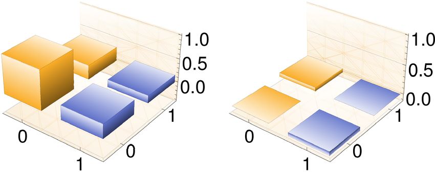
Figure 7. Theoretical and experimental reconstructed assemblages for different values of inputs x, y and outputs a, b, as mentioned in
Methods. Colors are for visualization purposes only. Each box shows the joint probability of measurement for the black boxes, real (top
left) and imaginary (top right) parts of the experimental density matrix of Charlie’s partition, and real (bottom left) and imaginary (bottom
right) parts of theoretical Charlie’s density matrix. The theoretical probability is 0.25 for all measurement choices and measurement outputs.You can also read