DISTRIBUTIONAL GENERALIZATION: A NEW KIND OF GENERALIZATION - OpenReview
←
→
Page content transcription
If your browser does not render page correctly, please read the page content below
Under review as a conference paper at ICLR 2021

D ISTRIBUTIONAL G ENERALIZATION :
A N EW K IND OF G ENERALIZATION
 Anonymous authors
 Paper under double-blind review

                                              A BSTRACT

         We introduce a new notion of generalization— Distributional Generalization—
         which roughly states that outputs of a classifier at train and test time are close as
         distributions, as opposed to close in just their average error. For example, if we
         mislabel 30% of dogs as cats in the train set of CIFAR-10, then a ResNet trained to
         interpolation will in fact mislabel roughly 30% of dogs as cats on the test set as well,
         while leaving other classes unaffected. This behavior is not captured by classical
         generalization, which would only consider the average error and not the distribution
         of errors over the input domain. Our formal conjectures, which are much more
         general than this example, characterize the form of distributional generalization
         that can be expected in terms of problem parameters: model architecture, training
         procedure, number of samples, and data distribution. We give empirical evidence
         for these conjectures across a variety of domains in machine learning, including
         neural networks, kernel machines, and decision trees. Our results thus advance our
         understanding of interpolating classifiers.

1    I NTRODUCTION
We begin with an experiment motivating the need for a notion of generalization beyond test error.
Experiment 1. Consider a binary classification version of CIFAR-10, where CIFAR-10 images x
have binary labels Animal/Object. Take 50K samples from this distribution as a train set, but
apply the following label noise: flip the label of cats to Object with probability 30%. Now train
a WideResNet f to 0 train error on this train set. How does the trained classifier behave on test
samples? Options below:

      1. The test error is low across all classes, since there is only 3% label noise in the train set
      2. Test error is “spread” across the animal class, After all, the classifier is not explicitly told
         what a cat or a dog is, just that they are all animals.
      3. The classifier misclassifies roughly 30% of test cats as “objects”, but all other types of
         animals are largely unaffected.

In fact, reality is closest to option (3). Figure 1 shows the results of this experiment with a WideResNet.
The left panel shows the joint density of train inputs x with train labels Object/Animal. Since
the classifier is interpolating, the classifier outputs on the train set are identical to the left panel. The
right panel shows the classifier predictions f (x) on test inputs x.

Figure 1: The setup and result of Experiment 1. The CIFAR-10 train set is labeled as either Animals
or Objects, with label noise affecting only cats. A WideResNet-28-10 is then trained to 0 train error
on this train set, and evaluated on the test set. Full experimental details are in C.2

                                                     1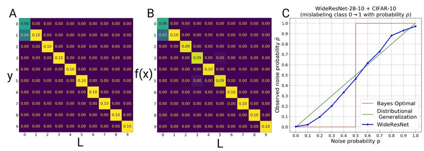
Under review as a conference paper at ICLR 2021

There are several notable things about this experiment. First, the error is localized to cats in test set
as it was in the train set, even though no explicit cat labels were provided. Second, the amount of
error on the cat class is close to the noise applied on the train set. Thus, the behavior of the classifier
on the train set generalizes to the test set in a certain sense. This type of similarity in behavior would
not be captured solely by average test error — it requires reasoning about the entire distribution of
classifier outputs. In our work, we show that this experiment is just one instance of a different type of
generalization, which we call “Distributional Generalization”. We now describe the mathematical
form of this generalization. Then, through extensive experiments, we will show that this type of
generalization occurs widely in existing machine learning methods: neural networks, kernel machines
and decision trees.

1.1   D ISTRIBUTIONAL G ENERALIZATION

Supervised learning aims to learn a model that correctly classifies inputs x ∈ X from a given
distribution D into classes y ∈ Y. We want a model with small test error on this distribution. In
practice, we find such a classifier by minimizing the train error of a model on the train set. This
procedure is justified when we expect a small generalization gap: the gap between the error on the
train and test set. That is, the trained model f should have: ErrorTrainSet (f ) ≈ ErrorTestSet (f ). We
now re-write this classical notion of generalization in a form better suited for our extension.
Classical Generalization: Let f be a trained classifier. Then f generalizes if:
                                E     [1{b
                                         y 6= y(x)}] ≈        E      [1{b
                                                                        y 6= y(x)}]                         (1)
                            x∼TrainSet                     x∼TestSet
                             b←f (x)
                             y                             b←f (x)
                                                           y

 Above, y(x) is the true class of x and yb is the predicted class. The LHS of Equation 1 is the train
error of f , and the RHS is the test error. Crucially, both sides of Equation 1 are expectations of the
same function (Terr (x, yb) := 1{by 6= y(x)}) under different distributions. The LHS of Equation 1
is the expectation of Terr under the “Train Distribution” Dtr , which is the distribution over (x, yb)
given by sampling a train point x along with its classifier-label f (x). Similarly, the RHS is under
the “Test Distribution” Dte , which is this same construction over the test set. These two distributions
are the central objects in our study, and are defined formally in Section 2.1. We can now introduce
Distributional Generalization, which is a property of trained classifiers. It is parameterized by a set of
bounded functions (“tests”): T ⊆ {T : X × Y → [0, 1]}.
Distributional Generalization: Let f be a trained classifier. Then f satisfies Distributional Gener-
alization with respect to tests T if:
                           ∀T ∈ T :           E     [T (x, yb)] ≈      E    [T (x, yb)]                     (2)
                                          x∼TrainSet                x∼TestSet
                                           b←f (x)
                                           y                        b←f (x)
                                                                    y

 We write this property as Dtr ≈T Dte . This states that the train and test distribution have similar
expectations for all functions in the family T . For the singleton set T = {Terr }, this is equivalent to
classical generalization, but it may hold for much larger sets T . For example in Experiment 1, the
train and test distributions match with respect to the test function “Fraction of true cats labeled as
object.” In fact, it is best to think of Distributional Generalization as stating that the distributions Dtr
and Dte are close as distributions.
This property becomes especially interesting for interpolating classifiers, which fit their train sets
exactly. Here, the Train Distribution (xi , f (xi )) is exactly equal1 to the original distribution (x, y) ∼
D, since f (xi ) = yi on the train set. In this case, distributional generalization claims that the
output distribution (x, f (x)) of the model on test samples is close to the true distribution (x, y). The
following conjecture specializes Distributional Generalization to interpolating classifiers, and will be
the main focus of our work.
Interpolating Indistinguishability Meta-Conjecture (informal): For interpolating classifiers f ,
and a large family T of test functions, the distributions:

                       (x, f (x))x∈TestSet ≈T (x, f (x))x∈TrainSet ≡ (x, y)x,y∼D
    1
      The formal definition of Train Distribution, in Section 2.1, includes the randomness of sampling the train
set as well. We consider a fixed train set in the Introduction for sake of exposition.

                                                       2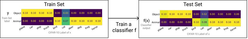
Under review as a conference paper at ICLR 2021

This is a “meta-conjecture”, which becomes a concrete conjecture once the family of tests T is
specified. One of the main contributions of our work is formally stating two concrete instances of this
conjecture— specifying exactly the family of tests T and their dependence on problem parameters
(the distribution, model family, training procedure, etc). It captures behaviors far more general than
Experiment 1, and applies to neural networks, kernels, and decision trees. We give empirical evidence
for conjectures across a variety of natural settings in machine learning.

1.2   S UMMARY OF C ONTRIBUTIONS

We extend the classical framework of generalization by introducing Distributional Generalization,
in which the train and test behavior of models are close as distributions. Informally, for trained
classifiers f , its outputs on the train set (x, f (x))x∈TrainSet are close in distribution to its outputs on
the test set (x, f (x))x∈TestSet , where the form of this closeness depends on specifics of the model,
training procedure, and distribution. This notion is more fine-grained than classical generalization,
since it considers the entire distribution of model outputs instead of just the test error.
We initiate the study of Distributional Generalization across various domains in machine learning.
For interpolating classifiers, we state two formal conjectures which predict the form of distributional
closeness that can be expected for a given model and task:
      1. Feature Calibration Conjecture (Section 3): Interpolating classifiers, when trained on sam-
         ples from a distribution, will match this distribution up to all “distinguishable features”
         (Definition 1).
      2. Agreement Conjecture (Section 4): For two interpolating classifiers of the same type, trained
         independently on the same distribution, their agreement probability with each other on test
         samples roughly matches their test accuracy.
We perform a number of experiments surrounding these conjectures, which reveal new behaviors
of standard interpolating classifiers (e.g. ResNets, MLPs, kernels, decision trees). We prove our
conjectures for 1-Nearest-Neighbors (Theorem 1), which suggests some form of “locality” as the
underlying mechanism. Finally, we discuss extending these results to non-interpolating methods in
Section 5. Our experiments and conjectures shed new light on the structure of interpolating classifiers,
which are extensively studied in recent years yet still poorly understood.
Related Work. Our work is inspired by the broader study of interpolating and overparameterized
methods in machine learning (e.g. Zhang et al. (2016); Belkin et al. (2018a;b; 2019); Liang and
Rakhlin (2018); Nakkiran et al. (2020); Schapire et al. (1998); Breiman (1995)). In a similar vein
to our work, Wyner et al. (2017); Olson and Wyner (2018) investigate decision trees, and show that
random forests are equivalent to a Nadaraya–Watson smoother (Nadaraya, 1964; Watson, 1964) with
a certain smoothing kernel. Our conjectures also describe neural networks under label noise, which
has been empirically and theoretically studied in the past (Zhang et al., 2016; Belkin et al., 2018b;
Rolnick et al., 2017; Natarajan et al., 2013; Thulasidasan et al., 2019; Ziyin et al., 2020; Chatterji
and Long, 2020), though not formally characterized. The behaviors we consider are also similar to
conditional density estimation (e.g. Tsybakov (2008); Dutordoir et al. (2018)), though we consider
samplers, not density estimators. We include a full discussion of related works in Appendix A.

2     P RELIMINARIES
Notation. We consider joint distributions D on x ∈ X and discrete y ∈ Y = [k]. Let Dn denote n iid
samples from D and S = {(xi , yi )} denote a train set. Let F denote the classifier family (including
architecture and training algorithm for neural networks), and let f ← TrainF (S) denote training
a classifier f ∈ F on train-set S. We consider classifiers which output hard decisions f : X → Y.
Let NNS (x) = xi denote the nearest-neighbor to x in train-set S, with respect to a distance metric
                                                                                                (y)
d. Our theorems will apply to any distance metric, and so we leave this unspecified. Let NNS (x)
                                                         (y)
denote the nearest-neighbor estimator itself, that is, NNS (x) := yi where xi = NNS (x).
Experimental Setup. Full experimental details are provided in Appendix B. Briefly, we train all
classifiers to interpolation (to 0 train error). Neural networks (MLPs and ResNets (He et al., 2016))

                                                     3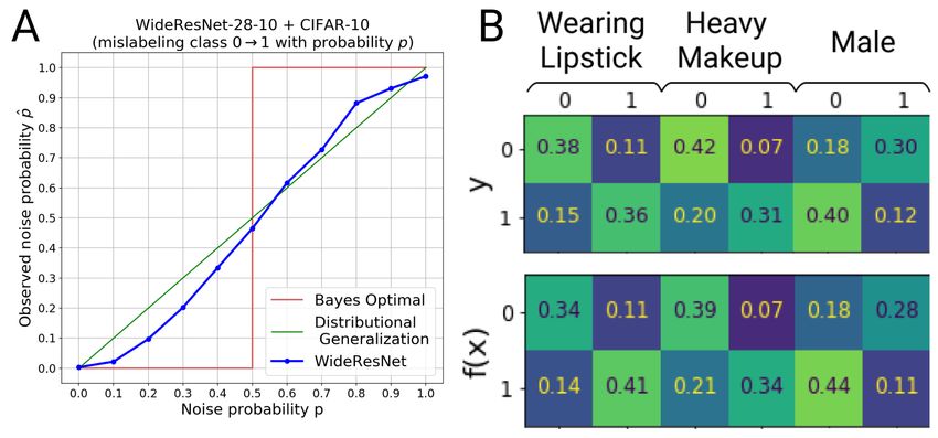
Under review as a conference paper at ICLR 2021

are trained with SGD. Interpolating decision trees are trained using the growth rule from Random
Forests (Breiman, 2001). For kernel classification, we consider kernel regression on one-hot labels
and kernel SVM, with small or 0 of regularization (which is often optimal Shankar et al. (2020)).
Distributional Closeness. We consider the following notion of closeness for two probability dis-
tributions: For two distributions P, Q over X × Y, let a “test” (or “distinguisher”) be a function
T : X × Y → [0, 1] which accepts a sample from either distribution, and is intended to classify the
sample as either from distribution P or Q. For any set C ⊆ {T : X × Y → [0, 1]} of tests, we say
distributions P and Q are “ε-indistinguishable up to C-tests” if they are close with respect to all tests
in class C. That is,

                    P ≈Cε Q ⇐⇒            sup       E    [T (x, y)] −      E    [T (x, y)] ≤ ε                     (3)
                                          T ∈C (x,y)∼P                  (x,y)∼Q

Total-Variation distance is equivalent to closeness in all tests, i.e. C = {T : X × Y → [0, 1]}, but we
consider closeness for restricted families of tests C. P ≈ε Q denotes ε-closeness in TV-distance.

2.1    F RAMEWORK FOR I NDISTINGUISHABILITY

We consider throughout the following three distributions over X × Y:

    Source D: (x, y)                      Train Dtr : (xtr , f (xtr ))          Test Dte (x, f (x))
    where x, y ∼ D                        S ∼ Dn , f ← TrainF (S),              S ∼ Dn , f ← TrainF (S),
                                          xtr , ytr ∼ S                         x, y ∼ D

The Source Distribution D is simply the original distribution. To sample from the Train Distribu-
tion Dtr , we first sample a train set S ∼ Dn , train a classifier f on it, then output (xtr , f (xtr )) for a
random train point xtr . That is, Dtr is the distribution of input and outputs of a trained classifier f
on its train set. To sample from the Test Distribution Dte , do we this same procedure, but output
(x, f (x)) for a random test point x. That is, the Dte is the distribution of input and outputs of a trained
classifier f at test time. The only difference between the Train Distribution and Test Distribution is
that the point x is sampled from the train set or the test set, respectively.2 For interpolating classifiers,
f (xtr ) = ytr on the train set, and so the Source and Train distributions are equivalent: D ≡ Dtr . Our
general thesis is that the Train and Test Distributions are indistinguishable under a variety of test
families T . Formally, we argue that for certain families of tests T and interpolating classifiers F, the
distributions: D ≡ Dtr ≈Tε Dte . Sections 3 and 4 give specific families of tests T for which these
distributions are indistinguishable.

3     F EATURE C ALIBRATION

The distributional closeness of Experiments 1 is subtle, and depends on the classifier architecture,
distribution, and training method. For example, Experiment 1 does not hold if we use a fully-
connected network (MLP) instead of a ResNet, or if we early-stop the ResNet instead of training
to interpolation (see Appendix C.2). Both these scenarios fail in different ways: An MLP cannot
properly distinguish cats even when trained on real CIFAR-10 labels, and so (informally) it has
no hope of behaving differently on cats in the setting of Experiment 1. On the other hand, an
early-stopped ResNet for Experiment 1 does not label 30% of cats as objects on the train set, since
it does not interpolate, and thus has no hope of reproducing this behavior on the test set. We now
characterize these behaviors, and their dependency on problem parameters, via a formal conjecture.
This conjecture characterizes a family of tests T for which the output distribution of a classifier
(x, f (x)) ∼ Dte is “close” to the source distribution (x, y) ∼ D. At a high level, we argue that
the distributions Dte and D are statistically close if we first “coarsen” the domain of x by some
labelling L : X → [M ]. That is, for certain partitions L, the following distributions are statistically
close: (L(x), f (x)) ≈ε (L(x), y). Intuitively, allowable partitions are those which can be learnt
from samples. To formalize the set of allowable partitions L for a training algorithm, we define a
    2
      Technically, these definitions require training a fresh classifier for each sample, using independent train sets.
We use this definition because we believe it is natural, although for practical reasons most of our experiments
train a single classifier f and evaluate it on the entire train/test set.

                                                          4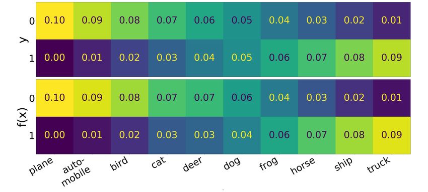
Under review as a conference paper at ICLR 2021

distinguishable feature: a partition of the domain X that is learnable for a given family of models.
For example, in Experiment 1, the partition into CIFAR-10 classes would be a distinguishable feature
for ResNets, but not for MLPs.
Definition 1 ((ε, F, D, n)-Distinguishable Feature). For a distribution D over X × Y, number of
samples n, family of models F, and small ε ≥ 0, an (ε, F, D, n)-distinguishable feature is a partition
L : X → [M ] of the domain X into M parts, such that training a model from F on n samples labeled
by L works to classify L with high test accuracy. Precisely, L is a (ε, F, D, n)-distinguishable feature
if:
                                      Pr           [f (x) = L(x)] ≥ 1 − ε
                            S={(xi ,L(xi )}x1 ,...,xn ∼D
                              f ←TrainF (S); x∼D

This definition depends only on the marginal distribution of D on x, and not on the label distribution
pD (y|x). To recap, this definition is meant to capture a labeling of the domain X that is learnable
for a given training procedure. It must depend on the classifier family F and number of samples
n, since more powerful classifiers can distinguish more features. Note that there could be many
distinguishable features for a given setting (ε, F, D, n) — including features not implied by the class
label such as the presence of grass in a CIFAR-10 image. Our main conjecture in this section is that
the test distribution (x, f (x)) ∼ Dte is statistically close to the source distribution (x, y) ∼ D when
the domain is “coarsened” by a distinguishable feature. Formally:
Conjecture 1 (Feature Calibration). For all natural distributions D, number of samples n, family
of interpolating models F, and ε ≥ 0, the following distributions are statistically close for all
(ε, F, D, n)-distinguishable features L:
                                    (L(x), f (x))          ≈ε   (L(x), y)                              (4)
                               f ←TrainF (D n ); x,y∼D            x,y∼D

We claim that this holds for all distinguishable features L “automatically” – we simply train a classifier,
without specifying any particular partition. As a trivial instance of the conjecture, suppose we have a
distribution with deterministic labels, and consider the ε-distinguishable feature L(x) := y(x), i.e.
the label itself. The ε here is then simply the test error of f , and Conjecture 1 is true by definition.
The formal statements of Definition 1 and Conjecture 1 may seem somewhat arbitrary, involving
many quantifiers over (ε, F, D, n). However, we believe these statements are natural. To support this,
in Theorem 1 we prove that Conjecture 1 is formally true as stated for 1-Nearest-Neighbor classifiers.
Connection to Indistinguishability. Conjecture 1 is an instantiation of our general Indistinguishably
Conjecture. In particular, Conjecture 1 is equivalent to the statement Dte ≈L     ε D where L is the
family of all tests which depend on x only via a distinguishable feature L. In other words, Dte is
indistinguishable from D to any function that only sees the input x via a distinguishable feature L(x).

3.1   E XPERIMENTS

We now give empirical evidence for our conjectures in a variety of settings in machine learning,
including neural networks, kernel machines, and decision trees. Selected experiments are summarized
here, with full details and further experiments in Appendix C.
Constant Partition: Consider the trivially-distinguishable constant feature L(x) = 0. Then, Con-
jecture 1 states that the marginal distribution of class labels for any interpolating classifier f (x) is
close to the true marginals p(y). We construct a variant of CIFAR-10 with class-imbalance and train
classifiers with varying levels of test errors (9-41%) to interpolation on it. The marginals of the
classifier outputs are close to that of the train set, irrespective of the test error. (See Appendix C.3).
Class Partition: We now consider settings where the original class labels form a distinguishable
feature (eg: CIFAR-10 classes are distinguishable by ResNets). The conjecture holds for arbitrary
distributions p(y|x). This includes the setting of Experiments 1 from the Introduction. We mislabel
class 0 → 1 with probability p in the CIFAR-10 train set and train a WideResNet-28-10 (WRN-28-10)
on this distribution. Now, we observe the fraction of samples mislabeled by this network pb from
0 → 1 in the test set. Figure 2 shows p versus pb. The Bayes optimal classifier for this distribution
behaves as a step function (in red), and a classifier that obeys Conjecture 1 exactly would follow the
diagonal (in green). The actual experiment (in blue) is close to the behavior predicted by Conjecture 1.

                                                       5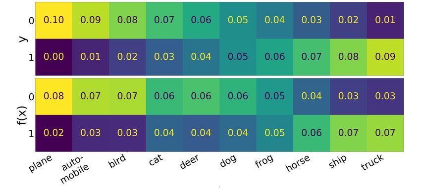
Under review as a conference paper at ICLR 2021

Appendix C.4 includes experiments for more distributions (including random joint density matrices)
and other classifiers such as Decisions Trees.
Multiple features: Conjecture 1 states that the network should be automatically calibrated for all
distinguishable features, without any explicit labels for them. To verify this, we use the CelebA
dataset (Liu et al., 2015), containing images with many binary attributes per image. We train a ResNet-
50 to classify one of the hard attributes (accuracy 80%) and confirm that the output distribution is
calibrated with respect to all attributes (Figure 2 that are themselves distinguishable by a ResNet-50.
Coarse Partition: Consider AlexNet trained on ILSVRC-2012 ImageNet (Russakovsky et al., 2015),
a 1000-class image classification problem with 116 varieties of dogs. The network achieves only
56.5% accuracy on the test set. But it will at least classify most dogs as dogs (with 98.4% accuracy),
making L(x) ∈ {dog, not-dog} a distinguishable feature. Per Conjecture 1, the network is calibrated
with respect to dogs: 22.4% of all dogs in ImageNet are Terriers, and the network classifies 20.9%
of all dogs as Terriers (though it has 9% error on which specific dogs it classifies as Terriers). See
Appendix Table 2 for details, and related experiments on ResNets and kernels in Appendix C.

                                                                            Figure 2: Feature Cali-
                                                                            bration. (A) CIFAR-10
                                                                            with p fraction of class
                                                                            0 → 1 mislabeled. Actual
                                                                            p vs. observed noise in the
                                                                            classifier outputs. (B) Mul-
                                                                            tiple feature calibration on
                                                                            CelebA.

3.2   D ISCUSSION

Conjecture 1 claims that Dte is close to D up to all tests which are themselves learnable. That is,
if an interpolating method is capable of learning a certain partition of the domain, then it will also
produce outputs that are calibrated with respect to this partition, when trained on any problem. This
conjecture thus gives a way of quantifying the resolution with which classifiers approximate the
source distribution D, via properties of the classification algorithm itself. This is in contrast to many
classical ways of quantifying the approximation of density estimators, which rely on analytic (rather
than operational) distributional assumptions (Tsybakov, 2008; Wasserman, 2006).
Proper Scoring Rules. If the loss function used in training is a strictly-proper scoring rule such
as cross-entropy (Gneiting and Raftery, 2007), then we may expect that in the limit of a large-
capacity network and infinite data, training on samples {(xi , yi )} will yield a good density estimate
of p(y|x) at the softmax layer. However, this is not what is happening in our experiments: First, our
experiments consider the hard-decisions, not the softmax outputs. Second, we observe Conjecture 1
even in settings without proper scoring rules (e.g. kernel SVM and decision trees).
1-Nearest-Neighbors Connection. Here we show that the 1-Nearest-Neighbor classifier provably
satisfies Conjecture 1, under mild assumptions. This theorem applies generically to a wide class
of distributions, with no assumptions on the ambient dimension of inputs or the underlying metric.
The only assumption is a weak regularity condition: sampling the nearest-neighbor train point to a
random test point should yield (close to) a uniformly random test point.
Theorem 1. Let D be a distribution over X × Y, and let n ∈ N be the number of train samples.
Assume the following regularity condition holds: Sampling the nearest-neighbor train point to a
random test point yields (close to) a uniformly random test point. That is, suppose that for some
small δ ≥ 0, the distributions: {NNS (x)}S∼Dn ≈δ {x}x∼D . Then, Conjecture 1 holds. That is,
                                            x∼D
for all (ε, NN, D, n)-distinguishable partitions L, the following distributions are statistically close:
                                                            (y)
                       {(y, L(x))}x,y∼D      ≈ε+δ       {(NNS (x), L(x)} S∼Dn                        (5)
                                                                           x,y∼D

                                                    6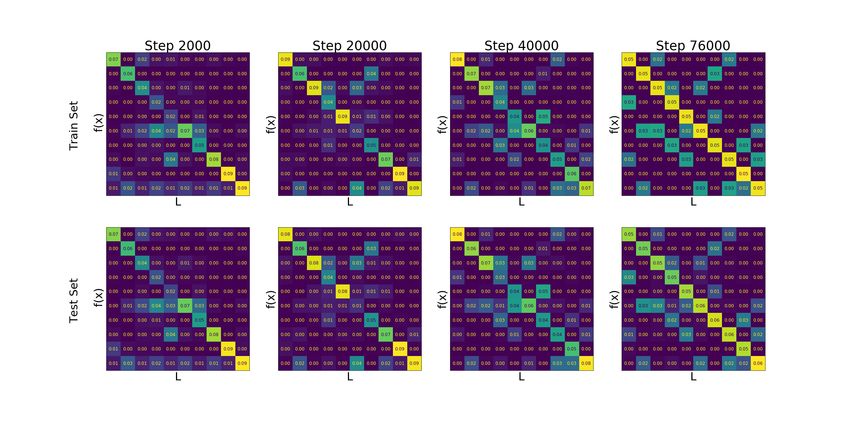
Under review as a conference paper at ICLR 2021

The proof of Theorem 1 is straightforward, and provided in Appendix E. We view this theorem both
as support for our formalism of Conjecture 1, and as evidence that the classifiers we consider in this
work have local properties similar to 1-Nearest-Neighbors.

4     AGREEMENT P ROPERTY
We now present an “agreement property” of interpolating classifiers. This property is independent of
the previous section, though both are special cases of our general indistinguishability conjecture. We
claim that, informally, the test accuracy of a classifier is close to the probability that it agrees with an
identically-trained classifier on a disjoint train set.
Conjecture 2 (Agreement Property). For certain classifier families F and distributions D, the test
accuracy of a classifier is close to its agreement probability with an independently-trained classifier.
That is, let S1 , S2 be disjoint train sets sampled from Dn , and let f1 , f2 be classifiers trained on
S1 , S2 respectively, then
                              Pr [f1 (x) = y] ≈          Pr [f1 (x) = f2 (x)]                           (6)
                               f1                       f1 ,f2
                            (x,y)∼D                   (x,y)∼D

Moreover, this holds with high probability over training f1 , f2 : Pr(x,y)∼D [f1 (x) = y] ≈
Pr(x,y)∼D [f1 (x) = f2 (x)].

The agreement property may be surprising for several reasons. For example, suppose we have two
classifiers f1 , f2 which were trained on independent train sets, and both achieve test accuracy say
50% on a 10-class problem. Depending on our intuition, we may expect (1) They agree with each
other much less than they agree with the true label, since each individual classifier is an independently
noisy version of the truth. OR (2) They agree with each other much more than 50%, since classifiers
tend to have “correlated” predictions. However, in practice there is a surprising coincidence, and they
agree with each other very close to 50%. Conjecture 2 also provably holds for 1-Nearest-Neighbors
in some settings, under stronger assumptions (Theorem 2 in Appendix E). Finally, in Section D.3, we
consider, and refute, several potential mechanisms which could explain the experimental results of
Conjecture 2.
Connection to Indistinguishability. Conjecture 2 is in fact a special case of our general Indistin-
guishability Conjecture. Formally, consider the specific test Tagree : (x, yb) 7→ 1{f1 (x) = yb} where
f1 ← TrainF (Dn ). The expectation of this test under the Source Distribution D is exactly the
LHS of Equation 6, while the expectation under the Test Distribution Dte is exactly the RHS. Thus,
Conjecture 2 can be equivalently stated as D ≈Tagree Dte .

4.1   E XPERIMENTS

In our experiments, we train a pair of
classifiers f1 , f2 on random disjoint
subsets of the train set for a given
distribution. Both classifiers are oth-
erwise trained identically, using the
same architecture, number of train-
samples n, and optimizer. We then
plot the test error of f1 against the
agreement probability Prx [f1 (x) =
f2 (x)]. Figure 3 shows experiments
with ResNet18 on CIFAR-10 and
CIFAR-100, with varying train sam-
ples n. The Agreement Property ap-           Figure 3: Agreement Property on CIFAR-10/100.
proximately holds for all pairs of iden-
tical classifiers, and continues to hold even for “weak” classifiers (e.g. when f1 , f2 have high test
error). Full experimental details are in Appendix D, including further experiments with RBF and
Laplace kernels, the Myrtle10 kernel (Shankar et al., 2020), and decision trees on UCI tasks.

                                                     7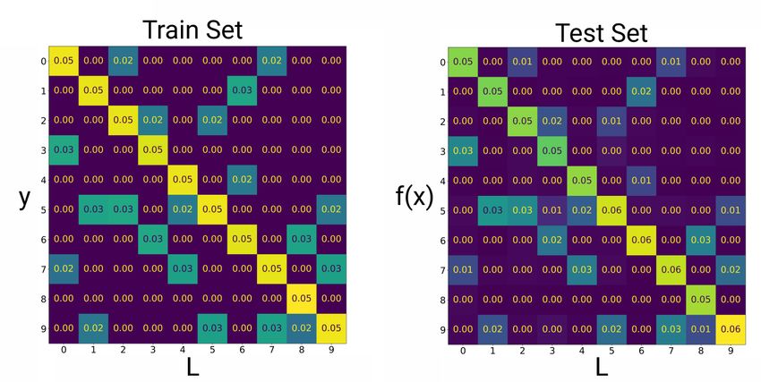
Under review as a conference paper at ICLR 2021
5 D ISTRIBUTIONAL G ENERALIZATION : B EYOND I NTERPOLATING M ETHODS
The previous sections have focused on interpolating classifiers,
which fit their train sets exactly. For non-interpolating classifiers,
their outputs on the train set (x, f (x))x∼TrainSet will not match the
original distribution (x, y) ∼ D. Thus, there is little hope that their
outputs on the test set will match the original distribution, and we
do not expect the Indistinguishability Conjecture to hold. How-
ever, Distributional Generalization does not require interpolation,
and we could still expect that the the train and test distributions are
close (Dtr ≈T Dte ) for some family of tests T . For example, the
following is a possible generalization of Feature Calibration.
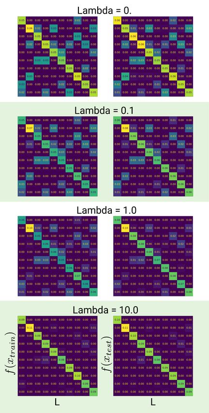
Conjecture 3 (Generalized Feature Calibration, informal). For
trained classifiers f , the following distributions are statistically
close for many partitions L of the domain:
(L(xi ), f (xi )) ≈ (L(x), f (x)) (7)
xi ∼TrainSet x∼TestSet
We leave unspecified the exact set of partitions L for which this
holds, since we do not yet understand the appropriate notion of “dis-
tinguishable feature” in this setting. However, we give experimental
evidence suggesting some refinement of Conjecture 3 is true. In
Figure 4 we train Gaussian kernel regression on MNIST, with label
noise determined by a random sparse confusion matrix. We vary the
`2 regularization, and plot the confusion matrix of predictions on the Figure 4: Distributional Gen-
train and test sets. With higher regularization, the kernel no longer eralization
interpolates the train set, but the test and train confusion matrices
remain close. That is, regularization prevents the kernel from fitting the noise on both the train and
test sets in a similar way. Full experimental details are given in Appendix B, including an analogous
experiment for neural networks on CIFAR-10, with early-stopping in place of regularization (Fig-
ure 22). These experiments suggests that Distributional Generalization is a meaningful notion even
for non-interpolating classifiers.
6 C ONCLUSION AND D ISCUSSION
In this work, we presented a new set of empirical behaviors of standard interpolating classifiers.
We unified these under the framework of Distributional Generalization, which states that outputs
of trained classifiers on the test set are “close” in distribution to their outputs on the train set. For
interpolating classifiers, we stated several formal conjectures (Conjectures 1 and 2) to characterize
the form of distributional closeness that can be expected.
Beyond Test Error. Our work proposes studying the entire distribution of classifier outputs on
test samples, beyond just its test error. We show that this distribution is often highly structured,
and we take steps towards characterizing it. Surprisingly, modern interpolating classifiers appear
to satisfy certain forms of distributional generalization “automatically,” despite being trained to
simply minimize train error. This even holds in cases when satisfying distributional generalization
is in conflict with satisfying classical generalization— that is, when a distributionally-generalizing
classifier must necessarily have high test error (e.g. Experiments 1 and 2). We thus hope that studying
distributional generalization will be useful to better understand modern classifiers, and to understand
generalization more broadly.
Classical Generalization. Our framework of Distributional Generalization can be insightful even to
study classical generalization. That is, even if we ultimately want to understand test error, it may be
easier to do so through distributional generalization. This is especially relevant for understanding the
success of interpolating methods, which pose challenges to classical theories of generalization. Our
work shows new empirical behaviors of interpolating classifiers, as well as conjectures characterizing
these behaviors. This sheds new light on these poorly understood methods, and could pave the way to
better understanding their generalization.
8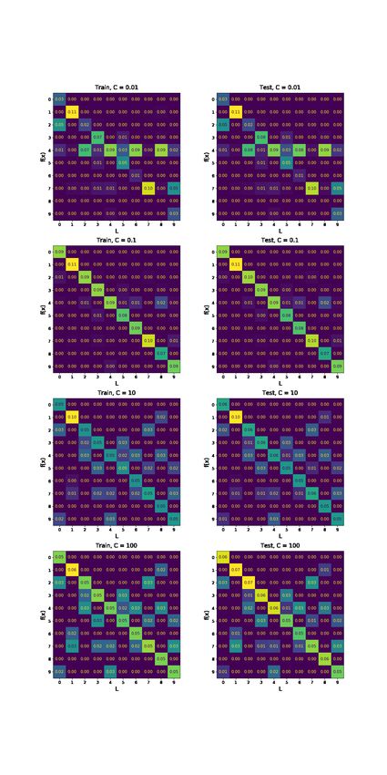
Under review as a conference paper at ICLR 2021

Interpolating vs. Non-interpolating Methods. Our work also suggests that interpolating classifiers
should be viewed as conceptually different objects from non-interpolating ones, even if both have
the same test error. In particular, an interpolating classifier will match certain aspects of the original
distribution, which a non-interpolating classifier will not. This also suggests, informally, that
interpolating methods should not be seen as methods which simply “memorize” their training data in
a naive way (as in a look up table) – rather this “memorization” strongly influences the classifier’s
decision boundary (as in 1-Nearest-Neighbors).
Limitations. The conjectures presented in this work are not fully specified, since they do not
exactly specify which classifiers or distributions for which they hold. We experimentally demonstrate
instances of these conjectures in various “natural” settings in machine learning, but we do not yet
understand which assumptions on the distribution or classifier are required. Some experiments also
deviate slightly from the predicted behavior. Nevertheless, we believe our conjectures capture the
essential aspects of the observed behaviors, at least to first order. It is an important open question to
refine these conjectures and better understand their applications and limitations— both theoretically
and experimentally.

6.1   O PEN Q UESTIONS

Our work raises a number of open questions and connections to other areas. We briefly collect some
of them here.

      1. As described in the limitations, we do not precisely understand the set of distributions and
         interpolating classifiers for which our conjectures hold. We empirically tested a number of
         “realistic” settings, but it is open to state formal assumptions defining these settings.
      2. It is open to theoretically prove versions of Distributional Generalization for models beyond
         1-Nearest-Neighbors. This is most interesting in cases where Distributional Generalization
         is at odds with classical generalization (e.g. Figure 2A).
      3. It is open to understand the mechanisms behind the Agreement Property (Section 4), theo-
         retically or empirically.
      4. There are a number of works suggesting “local” behavior of neural networks, and these
         are somewhat consistent with our locality intuitions in this work. However, it is open to
         formally understand whether these intuitions are justified in our setting.
      5. We give two families of tests T for which our Interpolating Indistinguishability Meta-
         conjecture empirically holds. This may not be exhaustive – there may be other ways in
         which the source distribution D and test distribution Dte are close. It is open to explore
         more ways in which Distributional Generalization holds, beyond the tests presented here.

R EFERENCES
Madhu S Advani and Andrew M Saxe. High-dimensional dynamics of generalization error in neural
 networks. arXiv preprint arXiv:1710.03667, 2017.
Zeyuan Allen-Zhu, Yuanzhi Li, and Yingyu Liang. Learning and generalization in overparameterized
  neural networks, going beyond two layers. In Advances in neural information processing systems,
  pages 6158–6169, 2019.
Sanjeev Arora, Simon Du, Wei Hu, Zhiyuan Li, and Ruosong Wang. Fine-grained analysis of
  optimization and generalization for overparameterized two-layer neural networks. In International
  Conference on Machine Learning, pages 322–332, 2019.
Susan Athey, Julie Tibshirani, Stefan Wager, et al. Generalized random forests. The Annals of
  Statistics, 47(2):1148–1178, 2019.
Francis Bach. Breaking the curse of dimensionality with convex neural networks. The Journal of
  Machine Learning Research, 18(1):629–681, 2017.
Peter L Bartlett, Philip M Long, Gábor Lugosi, and Alexander Tsigler. Benign overfitting in linear
  regression. Proceedings of the National Academy of Sciences, 2020.

                                                    9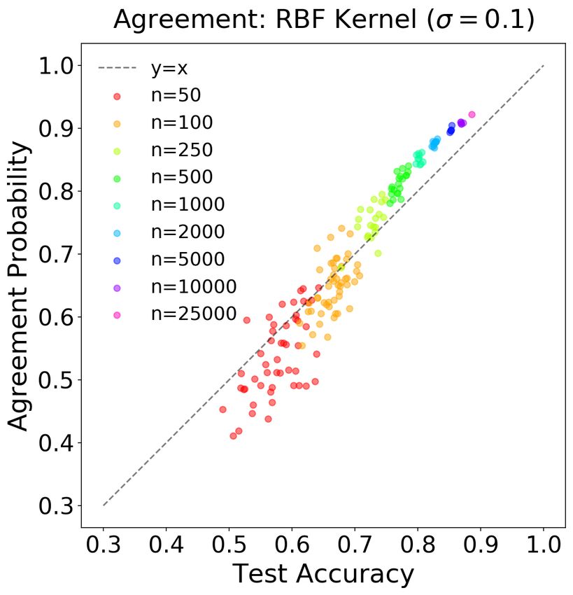
Under review as a conference paper at ICLR 2021

Mikhail Belkin, Daniel J Hsu, and Partha Mitra. Overfitting or perfect fitting? risk bounds for
 classification and regression rules that interpolate. In Advances in neural information processing
 systems, pages 2300–2311, 2018a.
Mikhail Belkin, Siyuan Ma, and Soumik Mandal. To understand deep learning we need to understand
 kernel learning. arXiv preprint arXiv:1802.01396, 2018b.
Mikhail Belkin, Daniel Hsu, Siyuan Ma, and Soumik Mandal. Reconciling modern machine-learning
 practice and the classical bias–variance trade-off. Proceedings of the National Academy of Sciences,
 116(32):15849–15854, 2019.
Leo Breiman. Reflections after refereeing papers for nips. The Mathematics of Generalization, pages
  11–15, 1995.
Leo Breiman. Random forests. Machine learning, 45(1):5–32, 2001.
Leo Breiman, Jerome Friedman, Charles J Stone, and Richard A Olshen. Classification and regression
  trees. CRC press, 1984.
Niladri S Chatterji and Philip M Long. Finite-sample analysis of interpolating linear classifiers in the
  overparameterized regime. arXiv preprint arXiv:2004.12019, 2020.
Lenaic Chizat and Francis Bach. Implicit bias of gradient descent for wide two-layer neural networks
  trained with the logistic loss. arXiv preprint arXiv:2002.04486, 2020.
Dheeru Dua and Casey Graff. UCI machine learning repository, 2017. URL http://archive.
  ics.uci.edu/ml.
Vincent Dutordoir, Hugh Salimbeni, James Hensman, and Marc Deisenroth. Gaussian process
  conditional density estimation. In Advances in neural information processing systems, pages
  2385–2395, 2018.
Gintare Karolina Dziugaite and Daniel M Roy. Computing nonvacuous generalization bounds for
  deep (stochastic) neural networks with many more parameters than training data. arXiv preprint
  arXiv:1703.11008, 2017.
Manuel Fernández-Delgado, Eva Cernadas, Senén Barro, and Dinani Amorim. Do we need hundreds
 of classifiers to solve real world classification problems? The journal of machine learning research,
 15(1):3133–3181, 2014.
Stanislav Fort, Paweł Krzysztof Nowak, Stanislaw Jastrzebski, and Srini Narayanan. Stiffness: A
  new perspective on generalization in neural networks. arXiv preprint arXiv:1901.09491, 2019.
Mario Geiger, Stefano Spigler, Stéphane d’Ascoli, Levent Sagun, Marco Baity-Jesi, Giulio Biroli,
 and Matthieu Wyart. Jamming transition as a paradigm to understand the loss landscape of deep
 neural networks. Physical Review E, 100(1):012115, 2019.
Federica Gerace, Bruno Loureiro, Florent Krzakala, Marc Mézard, and Lenka Zdeborová. Gener-
  alisation error in learning with random features and the hidden manifold model. arXiv preprint
  arXiv:2002.09339, 2020.
Behrooz Ghorbani, Song Mei, Theodor Misiakiewicz, and Andrea Montanari. Linearized two-layers
  neural networks in high dimension. arXiv preprint arXiv:1904.12191, 2019.
Tilmann Gneiting and Adrian E Raftery. Strictly proper scoring rules, prediction, and estimation.
  Journal of the American statistical Association, 102(477):359–378, 2007.
Sebastian Goldt, Madhu S Advani, Andrew M Saxe, Florent Krzakala, and Lenka Zdeborova.
  Generalisation dynamics of online learning in over-parameterised neural networks. arXiv preprint
  arXiv:1901.09085, 2019.
Chuan Guo, Geoff Pleiss, Yu Sun, and Kilian Q Weinberger. On calibration of modern neural
  networks. arXiv preprint arXiv:1706.04599, 2017.

                                                  10
Under review as a conference paper at ICLR 2021
Trevor Hastie, Robert Tibshirani, and Jerome Friedman. The elements of statistical learning: data
mining, inference, and prediction. Springer Science & Business Media, 2009.
Trevor Hastie, Andrea Montanari, Saharon Rosset, and Ryan J Tibshirani. Surprises in high-
dimensional ridgeless least squares interpolation. arXiv preprint arXiv:1903.08560, 2019.
Kaiming He, Xiangyu Zhang, Shaoqing Ren, and Jian Sun. Deep residual learning for image
recognition. In Proceedings of the IEEE conference on computer vision and pattern recognition,
pages 770–778, 2016.
Úrsula Hébert-Johnson, Michael Kim, Omer Reingold, and Guy Rothblum. Multicalibration: Cali-
bration for the (computationally-identifiable) masses. In International Conference on Machine
Learning, pages 1939–1948, 2018.
Tin Kam Ho. Random decision forests. In Proceedings of 3rd international conference on document
analysis and recognition, volume 1, pages 278–282. IEEE, 1995.
Rashidedin Jahandideh, Alireza Tavakoli Targhi, and Maryam Tahmasbi. Physical attribute prediction
using deep residual neural networks. arXiv preprint arXiv:1812.07857, 2018.
Alex Krizhevsky et al. Learning multiple layers of features from tiny images. 2009.
Balaji Lakshminarayanan, Alexander Pritzel, and Charles Blundell. Simple and scalable predictive
uncertainty estimation using deep ensembles. In Advances in neural information processing
systems, pages 6402–6413, 2017.
Yann LeCun, Léon Bottou, Yoshua Bengio, and Patrick Haffner. Gradient-based learning applied to
document recognition. Proceedings of the IEEE, 86(11):2278–2324, 1998.
Tengyuan Liang and Alexander Rakhlin. Just interpolate: Kernel” ridgeless” regression can generalize.
arXiv preprint arXiv:1808.00387, 2018.
Ziwei Liu, Ping Luo, Xiaogang Wang, and Xiaoou Tang. Deep learning face attributes in the wild. In
Proceedings of International Conference on Computer Vision (ICCV), December 2015.
Song Mei and Andrea Montanari. The generalization error of random features regression: Precise
asymptotics and double descent curve. arXiv preprint arXiv:1908.05355, 2019.
Nicolai Meinshausen. Quantile regression forests. Journal of Machine Learning Research, 7(Jun):
983–999, 2006.
Vidya Muthukumar, Kailas Vodrahalli, Vignesh Subramanian, and Anant Sahai. Harmless inter-
polation of noisy data in regression. IEEE Journal on Selected Areas in Information Theory,
2020.
Elizbar A Nadaraya. On estimating regression. Theory of Probability & Its Applications, 9(1):
141–142, 1964.
Vaishnavh Nagarajan and J. Zico Kolter. Uniform convergence may be unable to explain generaliza-
tion in deep learning, 2019.
Preetum Nakkiran, Gal Kaplun, Yamini Bansal, Tristan Yang, Boaz Barak, and Ilya Sutskever. Deep
double descent: Where bigger models and more data hurt. In International Conference on Learning
Representations, 2020.
Hariharan Narayanan and Sanjoy Mitter. Sample complexity of testing the manifold hypothesis. In
Advances in neural information processing systems, pages 1786–1794, 2010.
Nagarajan Natarajan, Inderjit S Dhillon, Pradeep K Ravikumar, and Ambuj Tewari. Learning with
noisy labels. In Advances in neural information processing systems, pages 1196–1204, 2013.
Brady Neal, Sarthak Mittal, Aristide Baratin, Vinayak Tantia, Matthew Scicluna, Simon Lacoste-
Julien, and Ioannis Mitliagkas. A modern take on the bias-variance tradeoff in neural networks.
arXiv preprint arXiv:1810.08591, 2018.
11Under review as a conference paper at ICLR 2021
Behnam Neyshabur, Zhiyuan Li, Srinadh Bhojanapalli, Yann LeCun, and Nathan Srebro. Towards
understanding the role of over-parametrization in generalization of neural networks. arXiv preprint
arXiv:1805.12076, 2018.
Alexandru Niculescu-Mizil and Rich Caruana. Predicting good probabilities with supervised learning.
In Proceedings of the 22nd international conference on Machine learning, pages 625–632, 2005.
Matthew A Olson and Abraham J Wyner. Making sense of random forest probabilities: a kernel
perspective. arXiv preprint arXiv:1812.05792, 2018.
Adam Paszke, Sam Gross, Soumith Chintala, Gregory Chanan, Edward Yang, Zachary DeVito,
Zeming Lin, Alban Desmaison, Luca Antiga, and Adam Lerer. Automatic differentiation in
pytorch. 2017.
F. Pedregosa, G. Varoquaux, A. Gramfort, V. Michel, B. Thirion, O. Grisel, M. Blondel, P. Pretten-
hofer, R. Weiss, V. Dubourg, J. Vanderplas, A. Passos, D. Cournapeau, M. Brucher, M. Perrot, and
E. Duchesnay. Scikit-learn: Machine learning in Python. Journal of Machine Learning Research,
12:2825–2830, 2011.
Taylor Pospisil and Ann B Lee. Rfcde: Random forests for conditional density estimation. arXiv
preprint arXiv:1804.05753, 2018.
Ali Rahimi and Benjamin Recht. Random features for large-scale kernel machines. In Advances in
neural information processing systems, pages 1177–1184, 2008.
David Rolnick, Andreas Veit, Serge Belongie, and Nir Shavit. Deep learning is robust to massive
label noise. arXiv preprint arXiv:1705.10694, 2017.
Jonas Rothfuss, Fabio Ferreira, Simon Walther, and Maxim Ulrich. Conditional density estimation
with neural networks: Best practices and benchmarks. arXiv preprint arXiv:1903.00954, 2019.
Olga Russakovsky, Jia Deng, Hao Su, Jonathan Krause, Sanjeev Satheesh, Sean Ma, Zhiheng Huang,
Andrej Karpathy, Aditya Khosla, Michael Bernstein, Alexander C. Berg, and Li Fei-Fei. ImageNet
Large Scale Visual Recognition Challenge. International Journal of Computer Vision (IJCV), 115
(3):211–252, 2015. doi: 10.1007/s11263-015-0816-y.
Robert E Schapire. Theoretical views of boosting. In European conference on computational learning
theory, pages 1–10. Springer, 1999.
Robert E Schapire, Yoav Freund, Peter Bartlett, Wee Sun Lee, et al. Boosting the margin: A new
explanation for the effectiveness of voting methods. The annals of statistics, 26(5):1651–1686,
1998.
Vaishaal Shankar, Alex Fang, Wenshuo Guo, Sara Fridovich-Keil, Ludwig Schmidt, Jonathan Ragan-
Kelley, and Benjamin Recht. Neural kernels without tangents. arXiv preprint arXiv:2003.02237,
2020.
Utkarsh Sharma and Jared Kaplan. A neural scaling law from the dimension of the data manifold.
arXiv preprint arXiv:2004.10802, 2020.
Sunil Thulasidasan, Tanmoy Bhattacharya, Jeff Bilmes, Gopinath Chennupati, and Jamal Mohd-
Yusof. Combating label noise in deep learning using abstention. arXiv preprint arXiv:1905.10964,
2019.
Alexandre B Tsybakov. Introduction to nonparametric estimation. Springer Science & Business
Media, 2008.
Pauli Virtanen, Ralf Gommers, Travis E. Oliphant, Matt Haberland, Tyler Reddy, David Cournapeau,
Evgeni Burovski, Pearu Peterson, Warren Weckesser, Jonathan Bright, Stéfan J. van der Walt,
Matthew Brett, Joshua Wilson, K. Jarrod Millman, Nikolay Mayorov, Andrew R. J. Nelson, Eric
Jones, Robert Kern, Eric Larson, CJ Carey, İlhan Polat, Yu Feng, Eric W. Moore, Jake Vand erPlas,
Denis Laxalde, Josef Perktold, Robert Cimrman, Ian Henriksen, E. A. Quintero, Charles R Harris,
Anne M. Archibald, Antônio H. Ribeiro, Fabian Pedregosa, Paul van Mulbregt, and SciPy 1. 0
Contributors. SciPy 1.0: Fundamental Algorithms for Scientific Computing in Python. Nature
Methods, 17:261–272, 2020. doi: https://doi.org/10.1038/s41592-019-0686-2.
12Under review as a conference paper at ICLR 2021
Larry Wasserman. All of nonparametric statistics. Springer Science & Business Media, 2006.
Geoffrey S Watson. Smooth regression analysis. Sankhyā: The Indian Journal of Statistics, Series A,
pages 359–372, 1964.
Abraham J Wyner, Matthew Olson, Justin Bleich, and David Mease. Explaining the success of
adaboost and random forests as interpolating classifiers. The Journal of Machine Learning
Research, 18(1):1558–1590, 2017.
Han Xiao, Kashif Rasul, and Roland Vollgraf. Fashion-mnist: a novel image dataset for benchmarking
machine learning algorithms. arXiv preprint arXiv:1708.07747, 2017.
Mohammad Yaghini, Bogdan Kulynych, and Carmela Troncoso. Disparate vulnerability: On the
unfairness of privacy attacks against machine learning. arXiv preprint arXiv:1906.00389, 2019.
Sergey Zagoruyko and Nikos Komodakis. Wide residual networks. arXiv preprint arXiv:1605.07146,
2016.
Chiyuan Zhang, Samy Bengio, Moritz Hardt, Benjamin Recht, and Oriol Vinyals. Understanding
deep learning requires rethinking generalization. arXiv preprint arXiv:1611.03530, 2016.
Liu Ziyin, Blair Chen, Ru Wang, Paul Pu Liang, Ruslan Salakhutdinov, Louis-Philippe Morency,
and Masahito Ueda. Learning not to learn in the presence of noisy labels. arXiv preprint
arXiv:2002.06541, 2020.
13Under review as a conference paper at ICLR 2021
A F ULL R ELATED W ORK
Our work is inspired by the broader study of interpolating and overparameterized methods in machine
learning; a partial list of works in this theme includes Zhang et al. (2016); Belkin et al. (2018a;b;
2019); Liang and Rakhlin (2018); Nakkiran et al. (2020); Mei and Montanari (2019); Schapire et al.
(1998); Breiman (1995); Ghorbani et al. (2019); Hastie et al. (2019); Bartlett et al. (2020); Advani
and Saxe (2017); Geiger et al. (2019); Gerace et al. (2020); Chizat and Bach (2020); Goldt et al.
(2019); Arora et al. (2019); Allen-Zhu et al. (2019); Neyshabur et al. (2018); Dziugaite and Roy
(2017); Muthukumar et al. (2020); Neal et al. (2018).
Interpolating Methods. Many of the best-performing techniques on high-dimensional tasks are
interpolating methods, which fit their train samples to 0 train error. This includes neural-networks
and kernels on images (He et al., 2016; Shankar et al., 2020), and random forests on tabular data
(Fernández-Delgado et al., 2014). Interpolating methods have been extensively studied both recently
and in the past, since we do not theoretically understand their practical success (Schapire et al., 1998;
Schapire, 1999; Breiman, 1995; Zhang et al., 2016; Belkin et al., 2018a;b; 2019; Liang and Rakhlin,
2018; Mei and Montanari, 2019; Hastie et al., 2019; Nakkiran et al., 2020). In particular, much of
the classical work in statistical learning theory (uniform convergence, VC-dimension, Rademacher
complexity, regularization, stability) fails to explain the success of interpolating methods (Zhang
et al., 2016; Belkin et al., 2018a;b; Nagarajan and Kolter, 2019). The few techniques which do apply
to interpolating methods (e.g. margin theory (Schapire et al., 1998)) remain vacuous on modern
neural-networks and kernels.
Decision Trees. In a similar vein to our work, Wyner et al. (2017); Olson and Wyner (2018)
investigate decision trees, and show that random forests are equivalent to a Nadaraya–Watson
smoother Nadaraya (1964); Watson (1964) with a certain smoothing kernel. Decision trees (Breiman
et al., 1984) are often intuitively thought of as “adaptive nearest-neighbors,” since they are explicitly
a spatial-partitioning method (Hastie et al., 2009). Thus, it may not be surprising that decision trees
behave similarly to 1-Nearest-Neighbors. Wyner et al. (2017); Olson and Wyner (2018) took steps
towards characterizing and understanding this behavior – in particular, Olson and Wyner (2018)
defines an equivalent smoothing kernel corresponding to a random forest, and empirically investigates
the quality of the conditional density estimate. Our work presents a formal characterization of the
quality of this conditional density estimate (Conjecture 1), which is a novel characterization even for
decision trees, as far as we know.
Kernel Smoothing. The term kernel regression is sometimes used in the literature to refer to kernel
smoothers, such as the Nadaraya–Watson kernel smoother (Nadaraya, 1964; Watson, 1964). But in
this work we use the term “kernel regression” to refer only to regression in a Reproducing Kernel
Hilbert Space, as described in the experimental details.
Label Noise. Our conjectures also describe the behavior of neural networks under label noise, which
has been empirically and theoretically studied in the past, though not formally characterized before
(Zhang et al., 2016; Belkin et al., 2018b; Rolnick et al., 2017; Natarajan et al., 2013; Thulasidasan
et al., 2019; Ziyin et al., 2020; Chatterji and Long, 2020). Prior works have noticed that vanilla
interpolating networks are sensitive to label noise (e.g. Figure 1 in Zhang et al. (2016), and Belkin
et al. (2018b)), and there are many works on making networks more robust to label noise via
modifications to the training procedure or objective (Rolnick et al., 2017; Natarajan et al., 2013;
Thulasidasan et al., 2019; Ziyin et al., 2020). In contrast, we claim this sensitivity to label noise is
not necessarily a problem to be fixed, but rather a consequence of a stronger property: distributional
generalization.
Conditional Density Estimation. Our density calibration property is similar to the guarantees of a
conditional density estimator. More specifically, Conjecture 1 states that an interpolating classifier
samples from a distribution approximating the conditional density of p(y|x) in a certain sense.
Conditional density estimation has been well-studied in classical nonparametric statistics (e.g. the
Nadaraya–Watson kernel smoother (Nadaraya, 1964; Watson, 1964)). However, these classical
methods behave poorly in high-dimensions, both in theory and in practice. There are some attempts
to extend these classical methods to modern high-dimentional problems via augmenting estimators
with neural networks (e.g. Rothfuss et al. (2019)). Random forests have also been known to exhibit
properties similar to conditional density estimators. This has been formalized in various ways, often
only with asymptotic guarantees (Meinshausen, 2006; Pospisil and Lee, 2018; Athey et al., 2019).
14Under review as a conference paper at ICLR 2021
No prior work that we are aware of attempts to characterize the quality of the resulting density
estimate via testable assumptions, as we do with our formulation of Conjecture 1. Finally, our
motivation is not to design good conditional density estimators, but rather to study properties of
interpolating classifiers — which we find happen to share properties of density estimators.
Uncertainty and Calibration. The Agreement Property (Conjecture 2) bears some resemblance to
uncertainty estimation (e.g. Lakshminarayanan et al. (2017)), since it estimates the the test error of a
classifier using an ensemble of 2 models trained on disjoint train sets. However, there are important
caveats: (1) Our Agreement Property only holds on-distribution, and degrades on off-distribution
inputs. Thus, it is not as helpful to estimate out-of-distribution errors. (2) It only gives an estimate of
the average test error, and does not imply pointwise calibration estimates for each sample.
Feature Calibration (Conjecture 1) is also related to the concepts of calibration and multicalibra-
tion (Guo et al., 2017; Niculescu-Mizil and Caruana, 2005; Hébert-Johnson et al., 2018). In our
framework, calibration is implied by Feature Calibration for a specific set of partitions L (determined
by level sets of the classifier’s confidence). However, we are not concerned with a specific set of
partitions (or “subgroups” in the algorithmic fairness literature) but we generally aim to characterize
for which partitions Feature Calibration holds. Moreover, we consider only hard-classification deci-
sions and not confidences, and we study only standard learning algorithms which are not given any
distinguished set of subgroups/partitions in advance. Our notion of distributional generalization is
also related to the notion of “distributional subgroup overfitting” introduced recently by Yaghini et al.
(2019) to study algorithmic fairness. This can be seen as studying distributional generalization for a
specific family of tests (determined by distinguished subgroups in the population).
Locality and Manifold Learning. Our intuition for the behaviors in this work is that they arise
due to some form of “locality” of the trained classifiers, in an appropriate space. This intuition is
present in various forms in the literature, for example: the so-called called “manifold hypothesis,”
that natural data lie on a low-dimensional manifold (e.g. Narayanan and Mitter (2010); Sharma and
Kaplan (2020)), as well as works on local stiffness of the loss landscape (Fort et al., 2019), and
works showing that overparameterized neural networks can learn hidden low-dimensional structure
in high-dimensional settings (Gerace et al., 2020; Bach, 2017; Chizat and Bach, 2020). It is open to
more formally understand connections between our work and the above.
B E XPERIMENTAL D ETAILS
Here we describe general background, and experimental details common to all sections. Then we
provide section-specific details below.
B.1 DATASETS
We consider the image datasets CIFAR-10 and CIFAR-100 (Krizhevsky et al., 2009), MNIST (LeCun
et al., 1998), Fashion-MNIST (Xiao et al., 2017), CelebA (Liu et al., 2015), and ImageNet (Rus-
sakovsky et al., 2015). We normalize images to x ∈ [0, 1]C×W ×H .
We also consider tabular datasets from the UCI repository Dua and Graff (2017). For UCI data, we
consider the 121 classification tasks as standardized in Fernández-Delgado et al. (2014). Some of these
tasks have very few examples, so we restrict to the 92 classification tasks from Fernández-Delgado
et al. (2014) which have at least 200 total examples.
B.2 M ODELS
We consider neural-networks, kernel methods, and decision trees.
B.2.1 D ECISION T REES
We train interpolating decision trees using a growth rule from
√ Random Forests (Breiman,
2001; Ho, 1995): selecting a split based on a random d subset of d features, split-
ting based on Gini impurity, and growing trees until all leafs have a single sam-
ple. This is as implemented by Scikit-learn Pedregosa et al. (2011) defaults with
RandomForestClassifier(n_estimators=1, bootstrap=False).
15You can also read